1.4 unit step & unit impulse...

CEN340: Signals and Systems; Ghulam Muhammad 1

1.4 Unit Step & Unit Impulse Functions

1.4.1 The Discrete-Time Unit Impulse and Unit-Step Sequences

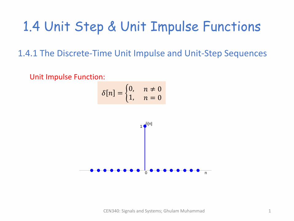
𝛿 𝑛 = ቊ0,1,

𝑛 ≠ 0𝑛 = 0

Unit Impulse Function:

Figure 1.28: Discrete-time Unit Impulse (sample)

0 n

1[n]


Unit Step & Unit Impulse

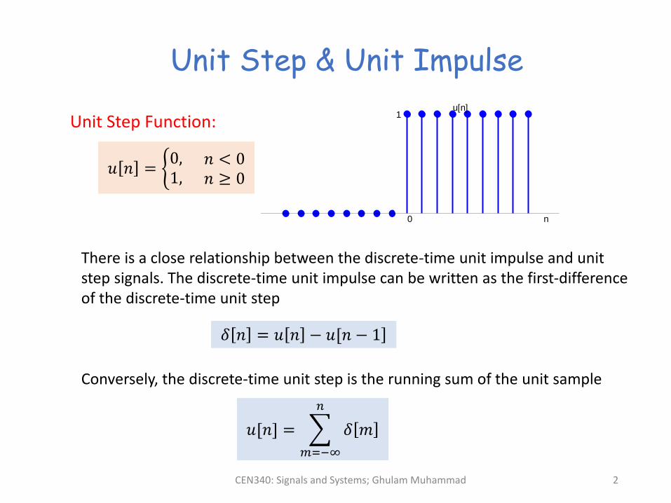
𝑢 𝑛 = ቊ0,1,

𝑛 < 0𝑛 ≥ 0

Unit Step Function:

Figure 1.29: Discrete-time Unit Step Sequence

0 n

1u[n]

There is a close relationship between the discrete-time unit impulse and unit step signals. The discrete-time unit impulse can be written as the first-difference of the discrete-time unit step

ሿ𝛿 𝑛 = 𝑢 𝑛 − 𝑢[𝑛 − 1

Conversely, the discrete-time unit step is the running sum of the unit sample

𝑢[𝑛ሿ =

𝑚=−∞

𝑛

𝛿 𝑚


Unit Step & Unit Impulse – contd.Figure 1.30 Running Sum of Eq. 1,66

0 m

[m]

Case (a): n < 0

n

Interval of summation

0 m

[m]

n

Case (b): n > 0

Interval of summation

0 for 𝑛 < 0 and 1 for 𝑛 ≥ 0

The unit impulse sequence can be used to sample the value of a signal at 𝑛 = 0.

In particular, since 𝛿 𝑛 is non-zero (and equal to 1) only for 𝑛 = 0, therefore

𝑥 𝑛 𝛿 𝑛 = 𝑥[0ሿ𝛿 𝑛

More generally, if we consider a unit impulse 𝛿 𝑛 − 𝑛0 at 𝑛 = 𝑛0, then

𝑥 𝑛 𝛿 𝑛 − 𝑛0 = 𝑥[𝑛0ሿ𝛿 𝑛 − 𝑛0


1.4.2 The Continuous-Time Unit Impulse and Unit-Step Sequences

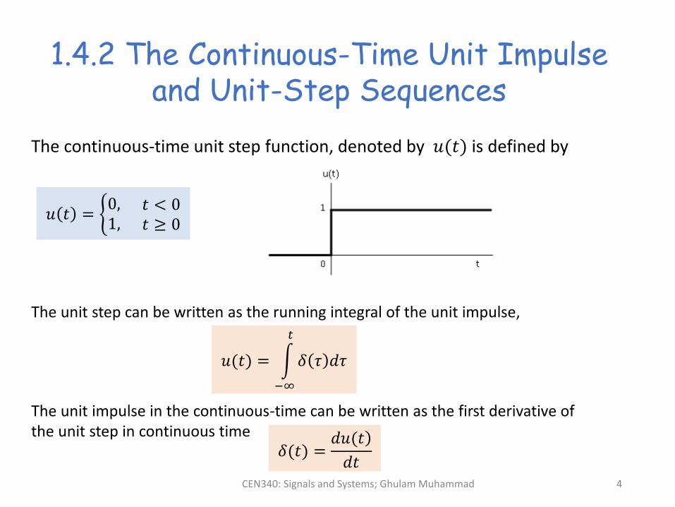
The continuous-time unit step function, denoted by 𝑢(𝑡) is defined by

𝑢 𝑡 = ቊ0,1,

𝑡 < 0𝑡 ≥ 0

The unit step can be written as the running integral of the unit impulse,

𝑢(𝑡) = න

−∞

𝑡

𝛿 𝜏 𝑑𝜏

The unit impulse in the continuous-time can be written as the first derivative of the unit step in continuous time

𝛿(𝑡) =)𝑑𝑢(𝑡

𝑑𝑡


We notice that u(t) is discontinuous at t=0 (and consequently cannot be differentiated at t=0), therefore, there is some formal difficulty with this equation in the previous slide.

The Continuous-Time Unit Impulse and Unit-Step Sequences

Therefore, we interpret equation by considering an approximation to the unit step 𝑢∆(𝑡) in which the function rises from 0 to 1 in a short time interval of length ∆. The step function 𝑢(𝑡) can be considered as an idealization of 𝑢∆(𝑡) for ∆ so short that its duration doesn’t matter for any practical purpose. More formally, 𝑢(𝑡) is the limit of 𝑢∆(𝑡) as ∆→ 0.

𝛿∆(𝑡) =)𝑑𝑢∆(𝑡

𝑑𝑡

Continuous-time approximation to the unit step function, 𝑢∆(𝑡)

Derivative of 𝑢∆(𝑡)


Continuous-Time Unit Impulse

It could be noticed that 𝛿∆(𝑡) is short pulse of duration ∆ and with unit area for any value of ∆. If we gradually decrease the value of ∆, the pulse will become narrower and the height will increase (to maintain the area to unity). Therefore, in the limiting case, we can write

𝛿 𝑡 = lim∆→0

𝛿∆ 𝑡

Continuous-time unit impulse Continuous-time scaled impulse

න𝜏=−∞

𝜏=𝑡

𝑘𝛿 𝜏 𝑑𝜏 = 𝑘𝑢(𝑡)

CEN340: Signals and Systems; Ghulam Muhammad

7

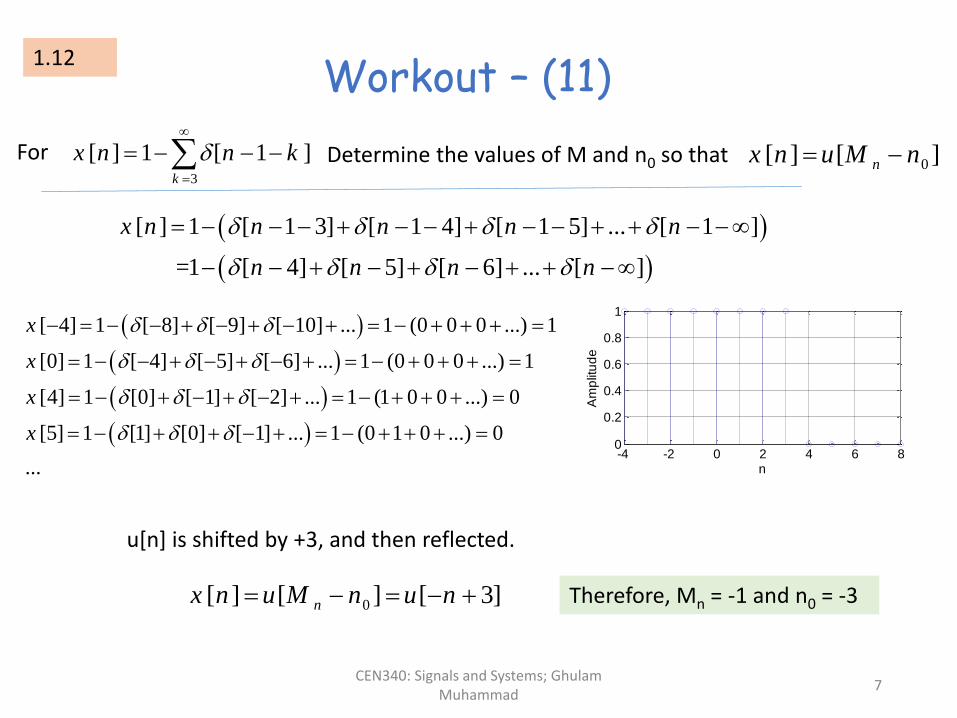
Workout – (11)1.12

3

[ ] 1 [ 1 ]k

x n n k

For Determine the values of M and n0 so that0[ ] [ ]nx n u M n

[ ] 1 [ 1 3] [ 1 4] [ 1 5] ... [ 1 ]

=1 [ 4] [ 5] [ 6] ... [ ]

x n n n n n

n n n n

[ 4] 1 [ 8] [ 9] [ 10] ... 1 (0 0 0 ...) 1

[0] 1 [ 4] [ 5] [ 6] ... 1 (0 0 0 ...) 1

[4] 1 [0] [ 1] [ 2] ... 1 (1 0 0 ...) 0

[5] 1 [1] [0] [ 1] ... 1 (0 1 0 ...) 0

...

x

x

x

x

-4 -2 0 2 4 6 80

0.2

0.4

0.6

0.8

1

n

Am

plit

ud

e

u[n] is shifted by +3, and then reflected.

0[ ] [ ] [ 3]nx n u M n u n Therefore, Mn = -1 and n0 = -3


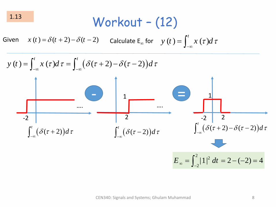
Workout – (12)1.13

( ) ( 2) ( 2)x t t t Given Calculate E for ( ) ( )t

y t x d

( ) ( ) ( 2) ( 2)t t

y t x d d

….

-2

( 2)t

d

….

2

( 2)t

d

2-2

( 2) ( 2)t

d

1 1

22

2|1| 2 ( 2) 4E dt

- =


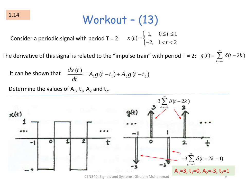
Workout – (13)1.14

Consider a periodic signal with period T = 2:1, 0 1

( )2, 1 2

tx t

t

The derivative of this signal is related to the “impulse train” with period T = 2: ( ) ( 2 )k

g t t k

It can be shown that1 1 2 2

( )( ) ( )

dx tA g t t A g t t

dt

Determine the values of A1, t1, A2 and t2.

3 ( 2 )k

t k

3 ( 2 1)k

t k

A1=3, t1=0, A2=-3, t2=1


1.5 Continuous-Time Discrete-Time Systems

A continuous-time system is a system in which continuous-time input signals are applied and result in continuous-time output signals. The input-output relation of such systems can be represented by the notation:

)𝑥(𝑡) → 𝑦(𝑡

Continuous-time system)𝑥(𝑡 )𝑦(𝑡

A discrete-time system is a system in which discrete-time input signals are applied

and result in discrete-time output signals. The input-output relation of such

systems can be represented by the notation:

ሿ𝑥[𝑛ሿ → 𝑦[𝑛

Continuous-time systemሿ𝑥[𝑛 ሿ𝑦[𝑛


Simple Example of Systems

A simple RC circuit with source VS

and capacitor voltage VC.

𝑖(𝑡) =)𝑣𝑠 𝑡 − 𝑣𝑐(𝑡

𝑅𝑖(𝑡) = 𝐶

)𝑑𝑣𝑐(𝑡

𝑑𝑡

)𝑑𝑣𝑐(𝑡

𝑑𝑡+

1

𝑅𝐶𝑣𝑐 𝑡 =

1

𝑅𝐶𝑣𝑠(𝑡)

The differential equation giving a relationship between the input 𝑣𝑠 𝑡 and the output 𝑣𝑐 𝑡 ,


Simple Example of Systems – contd.

An automobile responding to an applied force f from the engine and to a retarding force rvproportional to the automobile’s velocity v.

frv

Here we regard the force 𝑓(𝑡) as the input and velocity 𝑣(𝑡) as the output. If we let 𝑚 denote the mass of the automobile and 𝑚𝜌𝑣 the resistance due to friction, then equating acceleration i.e. the time derivative of velocity, with net force divided by mass, we get

)𝑑𝑣(𝑡

𝑑𝑡=

1

𝑚)𝑓 𝑡 − 𝜌𝑣(𝑡

)𝑑𝑣(𝑡

𝑑𝑡+𝜌

𝑚𝑣(𝑡) =

1

𝑚𝑓 𝑡


Example 1: Systems

As a simple example of a discrete-time system, consider a simple model for the balance in a bank account from month to month. Specifically, let 𝑦[𝑛ሿ denote the balance at the end of the n-th month, and suppose that 𝑦[𝑛ሿ evolves from month to month according to the equation

ሿ𝑦 𝑛 = 𝑦 𝑛 − 1 + 0.01𝑦[𝑛 − 1ሿ + 𝑥 𝑛 = 1.01𝑦[𝑛 − 1ሿ + 𝑥[𝑛

ሿ𝑦 𝑛 − 1.01𝑦 𝑛 − 1 = 𝑥[𝑛

Or,

Where 𝑥[𝑛ሿ represents the net deposit (i.e., deposits minus withdrawals) during

the month and the term 1.01𝑦[𝑛 − 1ሿ is the 1% profit each month.


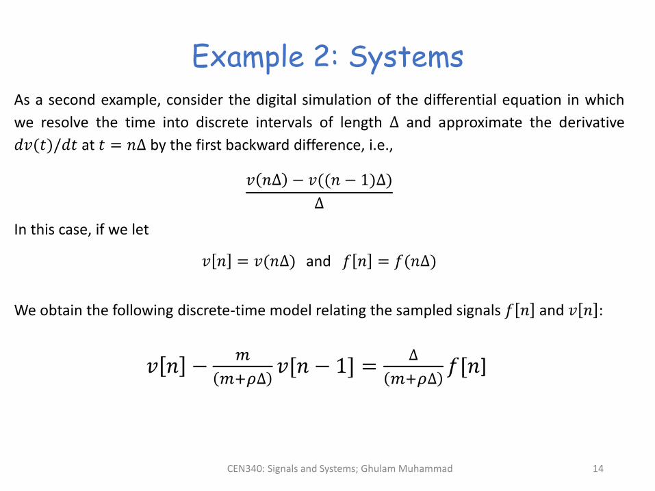
Example 2: SystemsAs a second example, consider the digital simulation of the differential equation in which

we resolve the time into discrete intervals of length ∆ and approximate the derivative

𝑑𝑣(𝑡)/𝑑𝑡 at 𝑡 = 𝑛∆ by the first backward difference, i.e.,

𝑣 𝑛∆ − 𝑣((𝑛 − 1)∆)

∆

In this case, if we let

𝑣 𝑛 = 𝑣(𝑛∆) and 𝑓 𝑛 = 𝑓(𝑛∆)

We obtain the following discrete-time model relating the sampled signals 𝑓 𝑛 and 𝑣 𝑛 :

𝑣 𝑛 −𝑚

𝑚+𝜌∆𝑣[𝑛 − 1ሿ =

∆

𝑚+𝜌∆𝑓[𝑛]


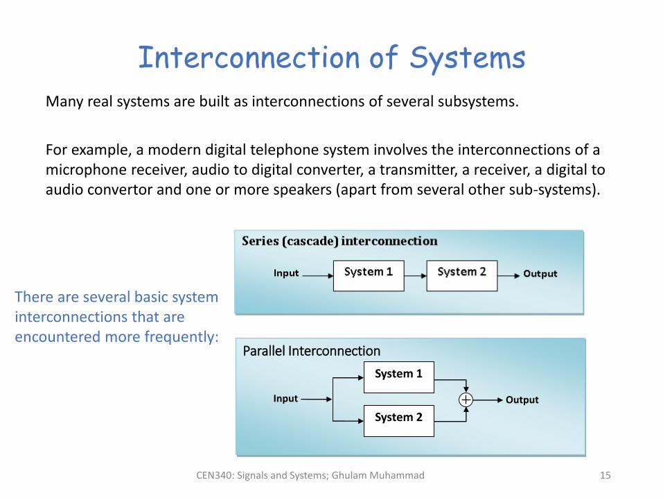
Interconnection of SystemsMany real systems are built as interconnections of several subsystems.

For example, a modern digital telephone system involves the interconnections of a microphone receiver, audio to digital converter, a transmitter, a receiver, a digital to audio convertor and one or more speakers (apart from several other sub-systems).

Parallel Interconnection

Input Output

System 1

System 2

There are several basic system interconnections that are encountered more frequently:


Interconnection of Systems – contd.

Feedback Interconnection


1.6 Basic System Properties

1.6.1 Systems with and without memory

A system is said to be memoryless if its output for each value of the independent variable at a given time is dependent on the input at only that same time.

For example, the system specified by the relationship

𝑦 𝑛 = 2𝑥 𝑛 − 𝑥2 𝑛 2

is memoryless, as the value of 𝑦 𝑛 at any particular time 𝑛0depends on the value of 𝑥 𝑛 only at that time, i.e. 𝑥 𝑛0 .

As a particular case, a resistor can be considered as a memoryless system: with the input 𝑥(𝑡) taken as the current and with voltage taken as the output 𝑦(𝑡), the input-output relationship for a resistor is,

)𝑦(𝑡) = 𝑅𝑥(𝑡

where 𝑅 is the resistance.


Systems with and without memory

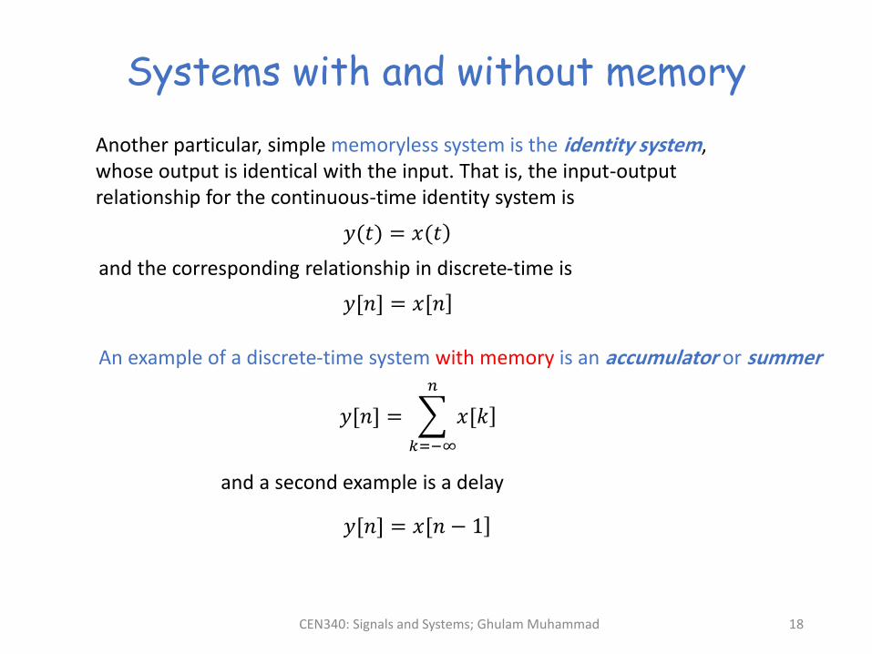
Another particular, simple memoryless system is the identity system, whose output is identical with the input. That is, the input-output relationship for the continuous-time identity system is

)𝑦(𝑡) = 𝑥(𝑡

and the corresponding relationship in discrete-time is

ሿ𝑦[𝑛ሿ = 𝑥[𝑛

An example of a discrete-time system with memory is an accumulator or summer

𝑦[𝑛ሿ =

𝑘=−∞

𝑛

ሿ𝑥[𝑘

and a second example is a delay

ሿ𝑦[𝑛ሿ = 𝑥[𝑛 − 1


A capacitor is an example of a continuous-time system with memory; since if the input is taken to be the current and the output is the voltage, then

Systems with memory

𝑦(𝑡) =1

𝐶න−∞

𝑡

𝑥(𝜏)𝑑𝜏

where 𝐶 is the capacitance

Delay Accumulator Storage of energy Memory dependent on the future values of the input and the output

Examples:


Invertibility and Inverse Systems

A system is said to be invertible if distinct inputs lead to distinct outputs.

Concept of an inverse system for a general invertible system

If a system is invertible, than an inverse system exists that, when cascaded with the original system, yields an output 𝑤 𝑛 equal to the input 𝑥 𝑛 to the first system.

)𝑦(𝑡) = 2𝑥(𝑡

𝑥(𝑡) =1

2𝑦(𝑡)

System

Inverse System


Example: Invertible SystemsAccumulator

Example: Non-invertible Systems

A system that produces a zero output sequence for any input sequence.

𝑦(𝑡) = 0

A system where the output is the square of the input.

)𝑦(𝑡) = 𝑥2(𝑡

The concept of invertibility is important in many applications. One particular example is that of systems used for encoding in a variety of communication systems.

Because, t = n will produce the same output.


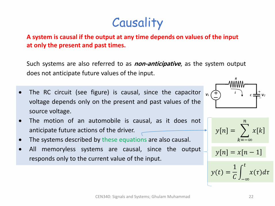
CausalityA system is causal if the output at any time depends on values of the input at only the present and past times.

Such systems are also referred to as non-anticipative, as the system output

does not anticipate future values of the input.

The RC circuit (see figure) is causal, since the capacitor

voltage depends only on the present and past values of the

source voltage.

The motion of an automobile is causal, as it does not

anticipate future actions of the driver.

The systems described by these equations are also causal.

All memoryless systems are causal, since the output

responds only to the current value of the input.

𝑦[𝑛ሿ =

𝑘=−∞

𝑛

ሿ𝑥[𝑘

ሿ𝑦[𝑛ሿ = 𝑥[𝑛 − 1

𝑦(𝑡) =1

𝐶න−∞

𝑡

𝑥(𝜏)𝑑𝜏


Causality – contd.

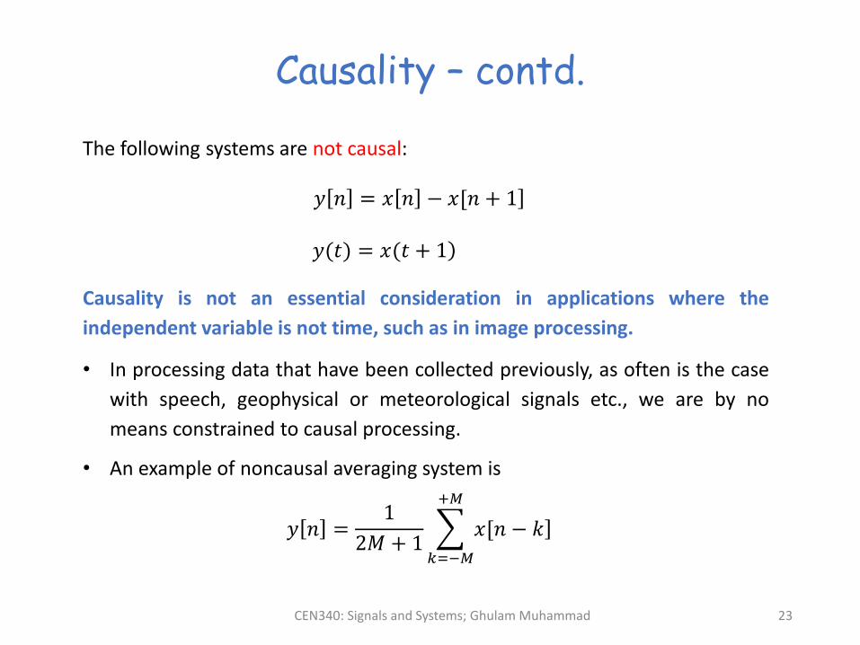
The following systems are not causal:

ሿ𝑦 𝑛 = 𝑥 𝑛 − 𝑥[𝑛 + 1

)𝑦(𝑡) = 𝑥(𝑡 + 1

Causality is not an essential consideration in applications where the

independent variable is not time, such as in image processing.

• In processing data that have been collected previously, as often is the case

with speech, geophysical or meteorological signals etc., we are by no

means constrained to causal processing.

• An example of noncausal averaging system is

𝑦 𝑛 =1

2𝑀 + 1

𝑘=−𝑀

+𝑀

ሿ𝑥[𝑛 − 𝑘


Causality – contd.

Consider the following system:

𝑦 𝑛 = 𝑥 −𝑛

Checking for the negative time, e.g. 𝑛 = −4, we see that 𝑦 −4 = 𝑥[4ሿ, so that the output at this time depends on a future value of the input. Hence the system is not causal.

Consider the following system:

𝑦(𝑡) = 𝑥 𝑡 co s( 𝑡 + 1)

In this system, the output at any time equals the input at that same time multiplied with a number that fluctuate with time. Specifically, we can re-write

𝑦(𝑡) = 𝑥 𝑡 g(t)

where g(t) is a time-varying function, namely g t = cos(t + 1). Thus, only the current value of the input influences the current value of the output, and we conclude that this system is causal (and, also memoryless).


Stability

A system is said to be stable if a small input leads to a response that does not diverge.

There are several examples of stable systems. “Stability of physical systems

generally results from the presence of mechanisms that dissipate energy”.

For example, in the RC circuit shown before, the resistor dissipates energy and this

circuit is a stable system.

More specifically,

If the input to a stable system is bounded (i.e., if its magnitude does not grow without bounds), then the output must also be bounded, and therefore cannot diverge.


Stability – contd.

𝑦 𝑛 =1

2𝑀 + 1

𝑘=−𝑀

+𝑀

ሿ𝑥[𝑛 − 𝑘

If the input 𝑥[𝑛ሿ to the system is bounded (say by a number 𝑩), for all values of 𝑛, then according to Equation above, the output 𝑦[𝑛ሿ of the system is also bounded by 𝑩. This is because the output 𝑦[𝑛ሿ is the average of a finite set of values of the input. Therefore, the output 𝑦[𝑛ሿ is bounded and the system is stable.

𝑦[𝑛ሿ =

𝑘=−∞

𝑛

ሿ𝑥[𝑘

This systems sums all of the past values of the input rather than just a finite set of values, and the system is unstable, since the sun can grow even if the input 𝑥[𝑛ሿ is bounded.


Example: Stability

Suppose we suspect that a particular system is unstable, then a useful strategy is to look for a specific bounded input that leads to an unbounded output for that system.

)𝑆1: 𝑦 𝑡 = 𝑡𝑥(𝑡

𝑆2: 𝑦 𝑡 = 𝑒 )𝑥(𝑡

Now, for system 𝑆1, a constant input 𝑥(𝑡) = 1 yields 𝑦 𝑡 = 𝑡, which is unbounded: since no matter what finite constant input we pick, 𝑦(𝑡) will exceed that constant for some 𝑡. Therefore, the system 𝑆1 is unstable.

For system 𝑆2, let us the input 𝑥(𝑡) be bounded by a positive number 𝐵, i.e.

𝑥 𝑡 < 𝐵 −𝐵 < 𝑥 𝑡 < 𝐵 for all 𝑡.

Using the definition of 𝑆2, we can write 𝑒−𝐵 < 𝑦 𝑡 < 𝑒𝐵

The system 𝑆2 is therefore, stable.


Time Invariance

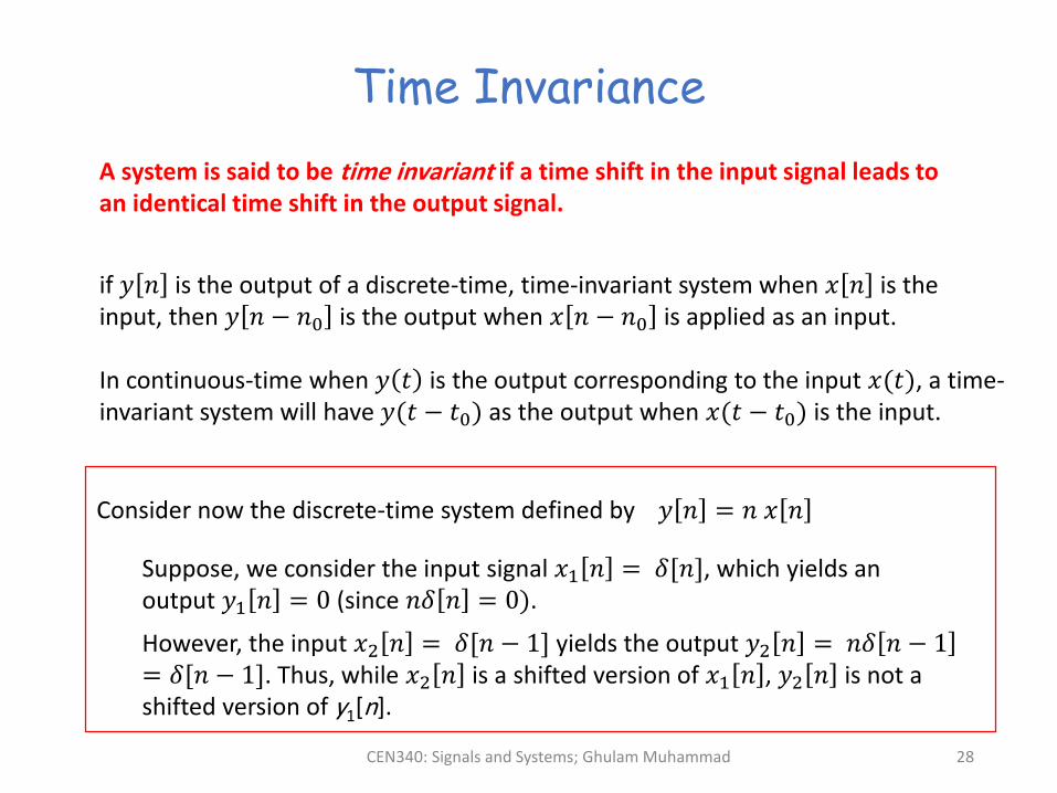
A system is said to be time invariant if a time shift in the input signal leads to an identical time shift in the output signal.

if 𝑦 𝑛 is the output of a discrete-time, time-invariant system when 𝑥 𝑛 is the input, then 𝑦 𝑛 − 𝑛0 is the output when 𝑥 𝑛 − 𝑛0 is applied as an input.

In continuous-time when 𝑦 𝑡 is the output corresponding to the input 𝑥(𝑡), a time-invariant system will have 𝑦(𝑡 − 𝑡0) as the output when 𝑥(𝑡 − 𝑡0) is the input.

Consider now the discrete-time system defined by 𝑦 𝑛 = 𝑛 𝑥 𝑛

Suppose, we consider the input signal 𝑥1 𝑛 = 𝛿[𝑛ሿ, which yields an output 𝑦1 𝑛 = 0 (since 𝑛𝛿 𝑛 = 0).

However, the input 𝑥2 𝑛 = 𝛿[𝑛 − 1ሿ yields the output 𝑦2 𝑛 = 𝑛𝛿 𝑛 − 1= 𝛿[𝑛 − 1ሿ. Thus, while 𝑥2 𝑛 is a shifted version of 𝑥1 𝑛 , 𝑦2 𝑛 is not a shifted version of y1[n].


Time Invariance – contd.

Consider the continuous-time system defined by 𝑦 𝑡 = si n )𝑥(𝑡

To check this system is time invariant, we must determine whether the time-invariance property holds for any input and any time shift 𝑡0. Thus, let 𝑥 𝑡 be an arbitrary input to this system, and let

𝑦1 𝑡 = si n )𝑥1(𝑡

to be the corresponding output. Then, consider a second input obtained by shifting 𝑥1(𝑡) in time

𝑥2 𝑡 = 𝑥1 𝑡 + 𝑡0

The corresponding output to this new input

𝑦2 𝑡 = sin 𝑥2 𝑡 = si n 𝑥1 𝑡 + 𝑡0

𝑦1 𝑡 + 𝑡0 = si n 𝑥1 𝑡 + 𝑡0

We see that 𝑦2 𝑡 = 𝑦1 𝑡 + 𝑡0 , and therefore, the system is time invariant.


Linearity

A linear system, in continuous-time or discrete-time, is a system that possesses the important property of superposition: If an input consists of the weighted sum of several signals, then the output is the superposition – that is, the weighted sum – of the responses of the system to each of those signals.

Let 𝑦1 𝑡 be the response of a continuous-time system to an input 𝑥1(𝑡), and

let 𝑦2 𝑡 be the response of a continuous-time system to an input 𝑥2(𝑡). Then the

system is linear if,

1. The response to 𝑥1 𝑡 + 𝑥2 𝑡 is 𝑦1 𝑡 + 𝑦2 𝑡 .

2. The response to 𝑎𝑥1 𝑡 is 𝑎𝑦1 𝑡 , where 𝑎 is any complex constant.

The first of these two properties is called the additivity property and the second

is known as the scaling or homogeneity property.

The two properties defining a linear system can be combined into a single statement:

𝑥1 𝑡 + 𝑏𝑥2 𝑡 = 𝑎𝑦1 𝑡 + 𝑏𝑦2 𝑡


Linearity – contd.

Additivity Homogeneity


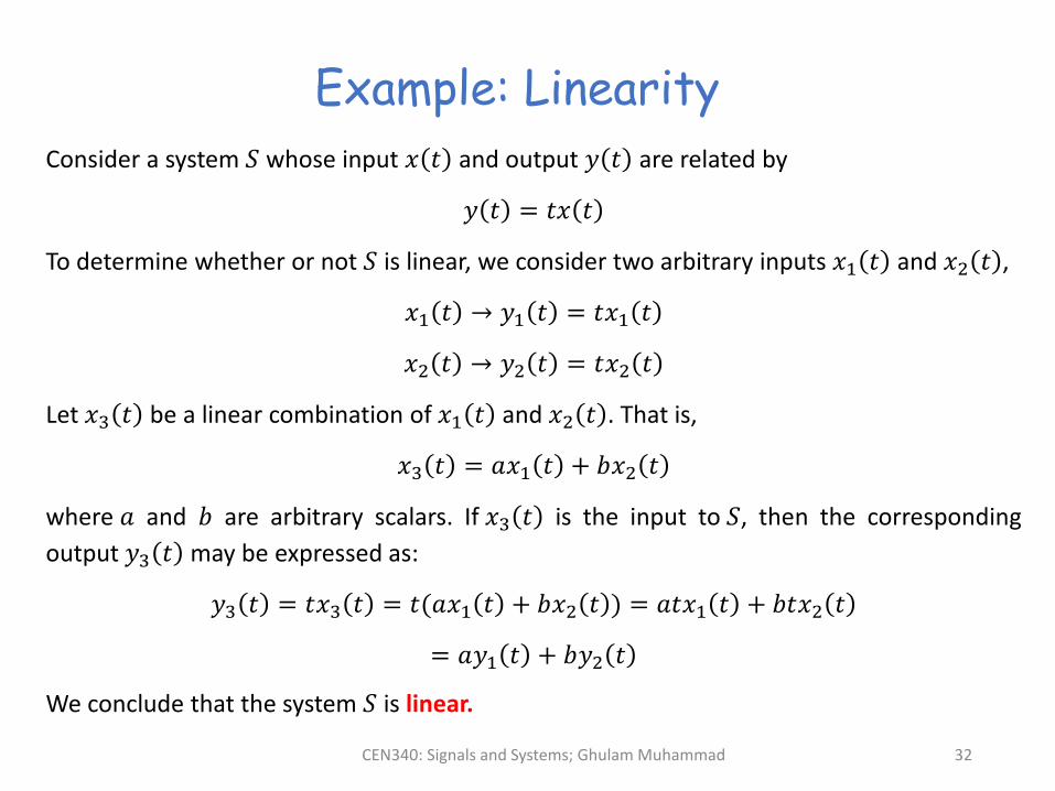
Example: Linearity

Consider a system 𝑆 whose input 𝑥 𝑡 and output 𝑦 𝑡 are related by

𝑦 𝑡 = 𝑡𝑥 𝑡

To determine whether or not 𝑆 is linear, we consider two arbitrary inputs 𝑥1 𝑡 and 𝑥2 𝑡 ,

𝑥1 𝑡 → 𝑦1 𝑡 = 𝑡𝑥1 𝑡

𝑥2 𝑡 → 𝑦2 𝑡 = 𝑡𝑥2 𝑡

Let 𝑥3 𝑡 be a linear combination of 𝑥1 𝑡 and 𝑥2 𝑡 . That is,

𝑥3 𝑡 = 𝑎𝑥1 𝑡 + 𝑏𝑥2 𝑡

where 𝑎 and 𝑏 are arbitrary scalars. If 𝑥3 𝑡 is the input to 𝑆, then the corresponding

output 𝑦3 𝑡 may be expressed as:

𝑦3 𝑡 = 𝑡𝑥3 𝑡 = 𝑡(𝑎𝑥1 𝑡 + 𝑏𝑥2 𝑡 ) = 𝑎𝑡𝑥1 𝑡 + 𝑏𝑡𝑥2 𝑡

= 𝑎𝑦1 𝑡 + 𝑏𝑦2 𝑡

We conclude that the system 𝑆 is linear.


Example: Linearity – contd.Let us now consider another system 𝑆 whose input 𝑥 𝑡 and output 𝑦 𝑡 are related by

𝑦 𝑡 = 𝑥2 𝑡

Like the previous example, to determine whether or not 𝑆 is linear, we consider two

arbitrary inputs 𝑥1 𝑡 and 𝑥2 𝑡 ,

𝑥1 𝑡 → 𝑦1 𝑡 = 𝑥12 𝑡

𝑥2 𝑡 → 𝑦2 𝑡 = 𝑥22 𝑡

Let 𝑥3 𝑡 be a linear combination of 𝑥1 𝑡 and 𝑥2 𝑡 . That is,

𝑥3 𝑡 = 𝑎𝑥1 𝑡 + 𝑏𝑥2 𝑡

where 𝑎 and 𝑏 are arbitrary scalars. If 𝑥3 𝑡 is the input to 𝑆, then the corresponding

output 𝑦3 𝑡 may be expressed as:

𝑦3 𝑡 = 𝑥32 𝑡 = 𝑎𝑥1 𝑡 + 𝑏𝑥2 𝑡

2= 𝑎2𝑥1

2 𝑡 + 𝑏2𝑥22 𝑡 + 2𝑎𝑏𝑥1 𝑡 𝑥2 𝑡

= 𝑎2𝑦1 𝑡 + 𝑏2𝑦2 𝑡 + 2𝑎𝑏𝑥1 𝑡 𝑥2 𝑡

Not Linear


Example: Linearity – contd.

While checking the linearity of a system, it is important to keep in mind that the system

must satisfy both the additivity and homogeneity properties and that the signals as well

the scaling constants are allowed to be complex.

𝑦 𝑛 = ℛ𝑒 𝑥 𝑛Consider: Additive Homogeneity ×

Let us assume, 𝑥1 𝑛 = 𝑟 𝑛 + 𝑗𝑠 𝑛

where 𝑟 𝑛 and 𝑠 𝑛 are the real and imaginary parts of the complex signal 𝑥 𝑛 , and that

the corresponding output is given by 𝑦1 𝑛 = 𝑟 𝑛

Now we consider the scaling of the complex input with a complex number say 𝑎 = 𝑗, i.e.

𝑥2 𝑛 = 𝑗𝑥1 𝑛 = 𝑗 𝑟 𝑛 + 𝑗𝑠 𝑛 = 𝑗𝑟 𝑛 − 𝑠 𝑛

Therefore, the corresponding output 𝑦2 𝑛 is given by 𝑦2 𝑛 = ℛ𝑒 𝑥2 𝑛 = −𝑠 𝑛

which is not equal to the scaled version of the 𝑦1 𝑛 : 𝑎𝑦1 𝑛 = 𝑗𝑟 𝑛

We conclude that the system violates the homogeneity property, therefore it is not linear.


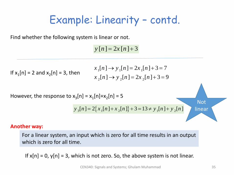
Example: Linearity – contd.

Find whether the following system is linear or not.

[ ] 2 [ ] 3y n x n

If x1[n] = 2 and x2[n] = 3, then1 1 1

2 2 2

[ ] [ ] 2 [ ] 3 7

[ ] [ ] 2 [ ] 3 9

x n y n x n

x n y n x n

However, the response to x3[n] = x1[n]+x2[n] = 5

3 1 2 1 2[ ] 2 [ ] [ ] 3 13 [ ] [ ]y n x n x n y n y n

Not linear

For a linear system, an input which is zero for all time results in an output which is zero for all time.

If x[n] = 0, y[n] = 3, which is not zero. So, the above system is not linear.

Another way:


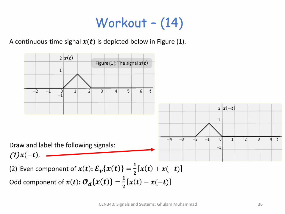
Workout – (14)A continuous-time signal 𝒙(𝒕) is depicted below in Figure (1).

Draw and label the following signals:

(1)𝒙 −𝒕 ,

(2) Even component of 𝒙 𝒕 : 𝓔𝒗 𝒙 𝒕 =𝟏

𝟐𝒙 𝒕 + 𝒙(−𝒕)

Odd component of 𝒙 𝒕 : 𝓞𝒅 𝒙 𝒕 =𝟏

𝟐𝒙 𝒕 − 𝒙(−𝒕)


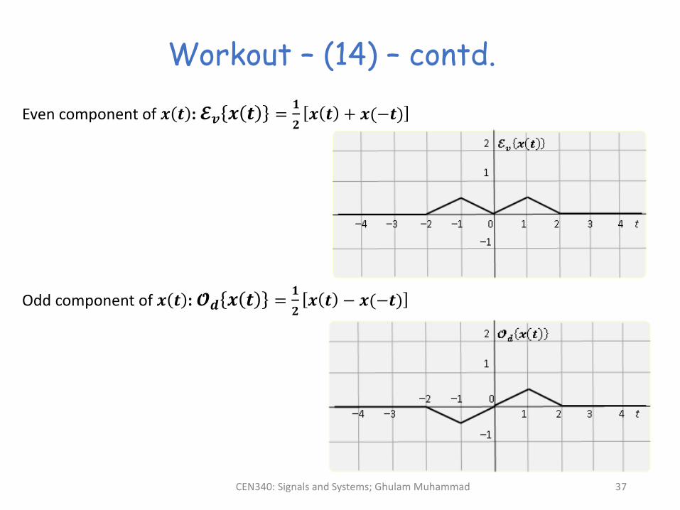
Workout – (14) – contd.

Even component of 𝒙 𝒕 : 𝓔𝒗 𝒙 𝒕 =𝟏

𝟐𝒙 𝒕 + 𝒙(−𝒕)

Odd component of 𝒙 𝒕 : 𝓞𝒅 𝒙 𝒕 =𝟏

𝟐𝒙 𝒕 − 𝒙(−𝒕)


Workout – (15)

-7 -6 -5 -4 -3 -2 -1 0 1 2 3 4 5 6 7-2

0

2

Original Signal

-7 -6 -5 -4 -3 -2 -1 0 1 2 3 4 5 6 7-2

0

2

x(t/2-2)

-7 -6 -5 -4 -3 -2 -1 0 1 2 3 4 5 6 7-2

0

2

x(-3t+5)

First, shift right by 2 samples. The first transition is now

shifted to (-1+2 =) 1. Then each position is multiplied by 2. So, 1 becomes (1x2 = ) 2.

First, shift left by 5 samples. The first

transition is now shifted to (-1-5 =) -6. Then each position is multiplied by 1/3. So, -6 becomes (-

6x1/3=) -2. Then, reflect. So -2 becomes 2.


44 ,4

2sin)(

tttx

Workout – (16)Drawing Sinusoids


Acknowledgement

The slides are prepared based on the following textbook:

• Alan V. Oppenheim, Alan S. Willsky, with S. Hamid Nawab, Signals & Systems, 2nd Edition, Prentice-Hall, Inc., 1997.

Special thanks to

• Prof. Anwar M. Mirza, former faculty member, College of Computer and Information Sciences, King Saud University

• Dr. Abdul Wadood Abdul Waheed, faculty member, College of Computer and Information Sciences, King Saud University

1.4 unit step & unit impulse...

Documents