13.12 simulation of the must field experiment

13.12 SIMULATION OF THE MUST FIELD EXPERIMENT USING

THE FEFLO-URBAN CFD MODEL

Fernando E. Camelli1*, Steven R. Hanna2, and Rainald Löhner1

1Laboratory for Computational Fluid Dynamics School of Computational Sciences

George Mason University, Fairfax, Virginia

2Hanna Consultants Kennebunkport, Maine

1. INTRODUCTION*

The validation of Computational Fluid Dynamics (CFD) models for the prediction of contaminant transport at urban scales has received a large amount of attention during the last decade (GMU 1997-2004). CFD models can provide a precise and detailed prediction of the wind and turbulence conditions needed to calculate the atmospheric transport and dispersion of chemical, biological or nuclear (CBN) agents. There have been several recent field and laboratory experiments involving flow and dispersion in urban areas or around arrays of obstacles, e.g. the Mock Urban Setting Test (MUST) (Biltoft 2001), Salt Lake City, and Oklahoma City, and wind or water tunnel experiments (Ejim 2002; Hall 1997; Macdonald et al. 2002; Macdonald et al. 2000; Yee et al. 2002). The focus of this paper is the MUST experiment that was carried out at Dugway Proving Ground. MUST was designed to represent an urban complex of about 100 buildings with symmetric characteristics. Sixty-eight puff and continuous releases were carried out in MUST using propylene as a tracer gas.

Two main CFD approaches are used to simulate transport and dispersion in the atmosphere at the urban scale: Reynolds Average Navier-Stokes Equation (RANS), and Large Eddy Simulation (LES). Both models lack accurate representation of turbulence. LES has limitations resolving the flow near the surface (Camelli et al. 2002). In some cases, RANS is not considered theoretically suitable for atmospheric flows (Wilcox 1998). As a response to some of these limitations, * Corresponding author address: Fernando E. Camelli, CFD Lab, MS 4C7, School of Computational Sciences, George Mason University, Fairfax, VA 22030; e-mail: [email protected]

variations to these models have surfaced in the last years, e.g. Very Large Eddy Simulation (VLES) (Camelli et al. 2004; Camelli et al. 2003), Detached Eddy Simulation (DES) (Forsythe et al. 2002), Monotonically Integrated Large Eddy Simulation (MILES) (Fureby et al. 2000, 2001; Grinstein et al. 2002), implicit turbulence modeling in LES (Margolin et al. 2002), hybrid LES/RANS (Camelli et al. 2002; Peltier et al. 2000). The spatial variations and unsteadiness of the flow in an urban setting have provided challenges to numerical modeling. In order to understand the importance of capturing these spatial variations and unsteadiness, the multipurpose finite element code FEFLO-URBAN was used to perform a Very Large Eddy Simulation (VLES) of MUST. Smagorinsky closure (Smagorinsky 1963) is used as the subgrid scale model. One of the continuous release trials (2682353) was selected for a detailed study. The terrain surface was modeled with geometric roughness in order to circumvent the lack of turbulence production in the vertical direction, which is a known problem for CFD modeling. The FEFLO-URBAN simulations for the concentration levels of the passive tracer were compared with the experimental measurements. Many possible measures of correlation can be devised. The present calculations were within an order of magnitude for 76% of all stations. A sensitivity study of the results with respect to mesh resolution and wind direction was performed.

The remainder of the paper is organized as follows: Section 2 describes the basis of CFD code, Section 3 the MUST experiment selected for comparison, Section 4 the mesh resolution study, Section 5 the comparison with experiment and Section 6 the sensitivity study with respect to wind direction. Some conclusions and outlook of future work are then given in Section 7.

2. MODEL DESCRIPTION 2.1 Time Integration

An explicit integration in time for the advective terms was used to capture the unsteadiness of the flow around the containers. Most of the diffusion in the atmosphere is due to the turbulent nature of the flow. The molecular diffusion is usually two orders of magnitude lower than the turbulent diffusion. Therefore, the time step selected for integration in time has to be small enough such that all the high frequencies that contribute to the turbulent diffusion are properly resolved in time. 2.2 Projection Scheme

The equations describing incompressible, Newtonian flows are written as

vvvv ∇∇=∇+∇+∂∂ µp

t (1)

0=⋅∇ v (2) Here p denotes the pressure, v the velocity vector and both the pressure p and the viscosity have been normalized by the (constant) density ρ. The important physical phenomena propagate with the advective timescales, i.e. with v. Diffusive phenomena typically occur at a much faster rate, and can/should therefore be integrated implicitly. Given that the pressure establishes itself immediately through the pressure-Poisson equation, an implicit integration of pressure is also required. The hyperbolic character of the advection operator and the elliptic character of the pressure-Poisson equation have led to a number of so-called projection schemes. The key idea is to predict first a velocity field from the current flow variables without taking the divergence constraint into account. In a second step, the divergence constraint is being separated into an advective-diffusive and pressure increment: ppann vvvvvv ∆+=∆+∆+=+ *1 (3) For an explicit integration of the advective terms (with implicit integration of the viscous terms), one complete time-step is given by: − Advective-Diffusive Prediction: *vv →n

( ) nnnnn pt

vvvvv ∇∇=∇+∇⋅+−

∇∇−∆

µµθ * 1(4)

− Pressure Correction: 1+→ nn pp 01 =⋅∇ +nv (5)

( ) 01*1

=−∇+∆− +

+nn

n

ppt

vv (6)

which results in

( )t

pp nn

∆⋅∇=−∇ +

*12 v

(7)

− Velocity Correction: 1* +→ nvv ( )nnn ppt −∇∆−= ++ 1*1 vv (8)

At steady state, 1* +== nn vvv and the residuals of the pressure correction vanish, implying that the results do not depend on the time-step t∆ . θ denotes the implicitness-factor for the viscous terms (θ=1.0: 1st order, fully implicit, θ=0.5: 2nd order, Cranck-Nicholson). This scheme has been widely used in conjunction with spatial discretization based on finite differences (Alessandrini et al. 1996; Bell et al. 1992; Bell et al. 1989; Kim et al. 1985), finite volumes (Kallinderis et al. 1996), and finite elements (Eaton 2001; Karbon et al. 2002; Löhner 1990; Löhner et al. 1999; Ramamurti et al. 1996). 2.3 Multi-stage Explicit Advective Prediction Scheme The scheme given by Equations (4-8) is, at best, of 2nd order in time. It is surprising to note that apparently no attempt has been made to use multistage explicit schemes to integrate the advective terms with higher order or to accelerate the convergence to steady state. This may stem from the fact that the implicit integration of viscous terms apparently impedes taking the full advantage multistage schemes offer for the Euler limit of no viscosity. An interesting alternative, used here, is to integrate with different time-stepping schemes in the different regimes of flows with highly variable cell Reynolds-number

µ

ρ hReh

v= (9)

For the case 1<hRe (viscous dominated), the accuracy in time is not important. However, for

1>hRe (advection dominated), the advantages of higher order time-marching schemes are considerable, particularly if one considers vortex transport over large distances. Dahlquist's theorem states that no unconditionally stable (implicit) scheme can be of order higher than two (this being the Cranck-Nicholson scheme). However, explicit schemes of the Runge-Kutta type can easily yield higher order time stepping. A k-step, time-accurate Runge-Kutta scheme for the advective parts may be written as:

( )1,1

111

0

−=∇∇+∇−∇⋅−

+=−−−

kip iniii

i

vvvvv

µγα (10)

( )

.

1

111 −−− ∇∇=∇+∇⋅

+−

∇∇−∆

knkk

nk

pt

vvv

vv

µ

µθ (11)

Here, the iα ’s are the standard Runge-Kutta coefficients, and θ is the implicitness-factor for the viscous terms (θ=1: 1st order, fully implicit, θ=0.5: 2nd order, Crank-Nicholson). The factor γ denotes the local ratio of the stability limit for explicit time stepping for the viscous terms versus the time-step chosen. Given that the advective and viscous time-step limits are proportional to:

;;2

µρhtht va ≈∆≈∆

v (12)

we immediately obtain ( ).,1min hRe=γ (13) In regions away from boundary layers, this factor is O(1), implying that a high-order Runge-Kutta scheme is recovered. Note that not using γ leads to schemes that are not of second order for the advective terms, unless an un-symmetric matrix is allowed on the left hand side. Besides higher accuracy, an important benefit of explicit multistage advection schemes is the larger time-step one can employ. The increase in allowable time-step is roughly proportional to the stages used. Given that most of the CPU time is spent solving the pressure-Poisson system (5), the

speedup achieved is also roughly proportional to the stages used (Löhner 2004). 3. DESCRIPTON OF MUST EXPERIMENT AND

SIMULATION The MUST experiment was designed to represent an urban layout with symmetric characteristics. An array of 10 by 12 containers was placed at the U.S. Army Dugway Proving Ground Horizontal Grid test site in Utah (Biltoft 2001). Each container was 12.2 m long, 2.42 m wide and 2.54 m high. The geometry of the MUST simulation is presented in Figure 1. The dimensions of the computational domain are: 320 m in length, 280 m in width, and 50 m in height above the ground.

Figure 1: MUST – 10 by 12 containers.

The MUST experiment utilized propylene as

the tracer gas. The density of propylene (C3H6) is 1.769 kg/m3. The tracer gas was measured using fast-response photo ionization detectors (PDI). The detectors were distributed between four 6 m towers, one 32 m tower, and four lines of sampling. The towers provided information of the vertical profile, while the sampling lines provided lateral dispersion information. Figure 2 shows the sensor distribution. A total of 72 stations were used within the array area. Four sampling lines with sensors at 1.6 m above ground were placed in the streets between containers. Reading from right to left in Figure 2:

a) sampling line 1: sensors 1 to 12, b) sampling line 2: sensors 13 to 21, c) sampling line 3: sensors 22 to 30, d) sampling line 4: sensors 31 to 40.

Five towers with sensors were placed within the array area, one 32 m tower in the center and four 6 m towers located in each quadrant of the

array. In addition to the information collected inside the array area, meteorological stations were placed outside the array to measure wind profiles and temperature.

The MUST experiment produced 63 continuous releases and 5 trials with multiple puff releases. The experimental data was statistically analyzed to establish its quality. The trial 2682353 was selected because of its statistical quality. This case was a continuous release from the top of one of the container at a height of 5.2 m from the ground (see Figure 2).

Figure 2:

a) 500K

c) 8M

Figure 3: F

The MUST s

different volumdependency. T(500K), the secothe third has 8,fourth has 31

surface meshes for the four different resolutions are shown in Figure 3. The average element size ranges from 0.64 m to 2.73 m (see Table 1).

No. of elements rmin [m] rmax [m] rmean [m] 500K 0.54 19.23 2.73 4M 0.34 16.44 1.27 8M 0.18 16.96 0.88 31M 0.16 8.72 0.64

Table 1: Mesh statistics.

LES has shown limitations producing the right amount of turbulence close to the walls (Mason 1994; Piomelli 1999), therefore dispersion in the E

)

)

)

NW

Source and station loca

b) 4

d) 3

our different surface me

imulation was carriede meshes to stu

he first has 576,411nd has 3,988,500 elem267,552 elements (8M,790,582 elements (

Relea

N
vicinity of walls is poorly predicted most of the time. In simple cases like a flat terrain, e.g. Prairie Grass experiment (Barad 1958; Haugen 1959), the turbulence close to the surface is under-predicted and washed out in the vertical direction (Camelli et al. 2000). Hybrid RANS/LES methods SE SW give an alternative (Camelli et al. 2002) to
(a

(b

(c)

(d

circumvent this deficiency, but in some cases more resolution is required close to the surfaces. This not only increases the required number of elements, but also reduces the explicit time-step for time accurate integration. An attractive

se source

Wind

tion.

M

1M

shes.

out in four dy mesh elements ents (4M), ), and the

31M). The

alternative, used here, is to introduce a geometric disturbance on the surface related to the roughness height (z0). This procedure was found to work well in previous calculations for flat terrain cases. The ground surface in the MUST simulation was modeled with a geometric roughness with z0=0.01 m and λ=1.0 m.

4. MESH RESOLUTION STUDY

A series of VLES simulations were performed with the multi-stage explicit advective prediction scheme. The air density is 1.225 kg/m3, and the viscosity is 1.789x10-5 kg/m/s. The Reynolds number in the atmosphere ranges from 105 to 108 (Arya 1999). The Smagorinsky turbulence model (Smagorinsky 1963) was used. A Courant number of C=0.6 was used in the time integration in combination with 3 stages of Runge-Kutta. The approximate time-steps for the four mesh resolution cases are shown in Table 2. The time-steps shown in Table 2 permit the capture of most high frequencies responsible for the diffusion of the gases.

No. of elements ∆t [s]

500K 1.85x10-1

4M 6.47x10-2 8M 3.45x10-2 31M 3.13x10-2

Table 2: Time-steps.

A variable wind with logarithmic profile is imposed at the inflow boundary condition (Hanna et al. 2002). The flow-field is first run until the turbulent flow-field is established in the whole computational domain. After this initialization step, the continuous release begins lasting 15 minutes real time. The solution was integrated on an SGI 3800 shared memory machine at the Naval Research Laboratory and an SGI ALTIX at George Mason University.

a) At 1 m from ground.

b) At 16 m from ground.

Figure 4: Velocity components time histories.

Figure 4 shows the time histories of the velocity

components (u,v,w) from two different stations from the simulation using 31M elements. The first time history (Figure 4.a) is from a station at 1 m above the ground and the second (Figure 4.b) comes from a station at 16 m above the ground. Both stations are placed in the 32 m tower located at the geometric center of the array of containers

(see Figure 2). These plots show the turbulent behavior of the velocity components at two different heights, the station nearer the ground has higher frequency changes than the station up in the canopy.

Figure 5 shows cut planes for the absolute value of the velocity at 1.5 m and 5.2 m from the ground level. The average wind speed is between 0.0 and 1.3 m/s at 1.5 m from ground level (Figure 5.a) and about 4.1 m/s at the release height of 5.2 m (Figure 5.b). Recirculation regions are observed between containers with no unique pattern.

a) At 1.5 m from ground.

b) At 5.2 m from ground.

Figure 5: Cut plane of the instantaneous absolute velocity

Dispersion clouds for the 500K, 4M and 31M

cases are shown in Figure 6. In all the cases the clouds represent an iso-surface of concentration level at the same time (t=200 s). The cloud is short with no sign of recirculation for the 500K case (Figure 6.a). The cloud in the 4M case starts to

have a richer structure with some detached sub-clouds, covering a larger volume than the 500K case (see Figure 6.b). The cloud for the 31M case shows the most complex structure of all, with many sub-clouds, and the cover area is comparable with the 4M case cloud (Figure 6.c).

a) 500K

b) 4M

c) 31M.

Figure 6: Dispersion cloud at 200 s.

a) Plume footprint at a vertical cut-plane along the

wind direction.

b) Plume footprint at 5.2 m from ground.

Figure 7: Concentration footprint.

The plume footprint produced by the

continuous release is shown in Figure 7 with a scale that ranges from 0.0 to 8.16 ppm. The typical instantaneous meandering of plume produced by the continuous release is observed in Figure 7.b. This footprint is at the release height of 5.2 m. Figure 7.a shows the footprint in a cut-plane along the wind direction, the bottom of the plume takes a while to reach the ground. This may be because the vertical turbulence is underestimated.

A comparison was made with the concentration levels taken from the four numerical cases. The results can be seen in Figure 8 to Figure 15; these Figures do not show comparison with the experiment.

Figure 8: Concentration at sampling line 1.

In Figure 8, the concentration levels are

comparable for the 500K, 8M and 31M cases. An exception to this comparison was station 9 in the 500K case. This station showed the highest concentration level without any pattern. The 4M

case deviated from the others by giving multiple zero values. The values in sampling lines 2 (Figure 9), 3 (Figure 10), and 4 (Figure 11) are all comparable among the different resolution cases.




Figure 12 to Figure 15 show the time average

concentrations in the 32 m tower and in three 6 m towers. The remaining 6 m tower, in the NW quadrant with stations 49 to 54, is omitted because the averages from the simulation are all less than 10-14 ppm. These concentrations are close to zero and consistent with the experimental data. This tower is located in the outer region of the plume envelope.

Figure 12: Concentration at 31 m tower.

Figure 13: Concentration at SW 6 m tower.

Figure 14: Concentration at NE 6 m tower.

Figure 15: Concentration at SE 6 m tower.

5. COMPARISON WITH THE EXPERIMENT

The time history for station 31 from the 31M elements case is shown in Figure 16. The average concentration value for this station is 0.97 ppm with a standard deviation of 2.33 ppm. The maximum value is 30 ppm and many peaks in the range of 5 to 10 ppm are observed during the 15 minutes of numerical data collection. It is important to remark that sometimes the information provided by average values can be inconclusive. For example, Figure 16 shows the time history for a certain station with a time average of approximately 1 ppm. However, there are many peaks with values that greatly exceed that average value. It is certain that any agent dispersed in the atmosphere will present a time history that resembles Figure 16. Since some CBN agents can be deadly within a few seconds of a minimum level exposure, the information given by time averages can be erroneous, and may mislead any analysis based only on it. This scenario supports the use of LES (spatial filtering) over RANS (temporal filtering) to simulate atmospheric dispersion.

Figure 16: Concentration time history for station 31

The experimental data averages are compared with the averages of the 31M case in Figure 17 to

Figure 24. The numerical averages are each presented with bars representing the standard deviation of the time history for that given station. The numerical averages predicted or under-predicted the experimental results within 65%. If the standard deviation of the numerical averages is considered, the numerical averages hold within the experimental values 76%. The concentration levels outside the plume envelope (zero level) are all properly predicted: stations 10 to 12 in sampling line 1, stations 19 to 21 in sampling line 2, stations 25 to 30 in sampling line 3, and stations 33 to 40 in sampling line 4.

0.0

2.0

4.0

6.0

0 1 2 3 4 5 6 7 8 9 10 11 12 13

Station #c

[ppm

]

Exper.

31M run

Figure 17: Comparison between experiment and

31M at sampling line 1.

0.0

5.0

10.0

15.0

20.0

12 13 14 15 16 17 18 19 20 21 22

Station #

c [p

pm]

Exper.

31M run



0.0

2.0

4.0

6.0

21 22 23 24 25 26 27 28 29 30 31

Station #

c [p

pm]

Exper.

31M run



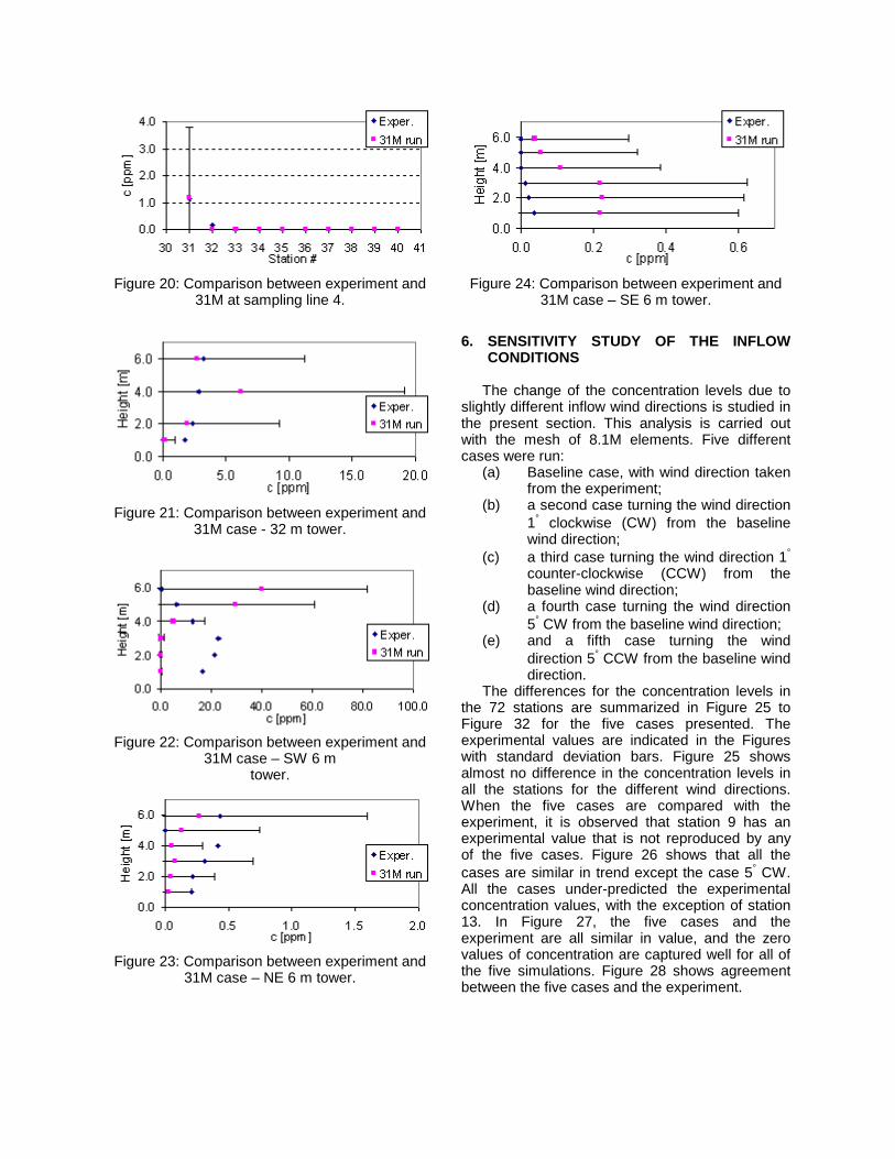
Figure 20: Comparison between experiment and 31M at sampling line 4.

Figure 21: Comparison between experiment and 31M case - 32 m tower.

Figure 22: Comparison between experiment and 31M case – SW 6 m

tower.

Figure 23: Comparison between experiment and 31M case – NE 6 m tower.

Figure 24: Comparison between experiment and 31M case – SE 6 m tower.

6. SENSITIVITY STUDY OF THE INFLOW

CONDITIONS

The change of the concentration levels due to slightly different inflow wind directions is studied in the present section. This analysis is carried out with the mesh of 8.1M elements. Five different cases were run:

(a) Baseline case, with wind direction taken from the experiment;

(b) a second case turning the wind direction 1° clockwise (CW) from the baseline wind direction;

(c) a third case turning the wind direction 1° counter-clockwise (CCW) from the baseline wind direction;

(d) a fourth case turning the wind direction 5° CW from the baseline wind direction;

(e) and a fifth case turning the wind direction 5° CCW from the baseline wind direction.

The differences for the concentration levels in the 72 stations are summarized in Figure 25 to Figure 32 for the five cases presented. The experimental values are indicated in the Figures with standard deviation bars. Figure 25 shows almost no difference in the concentration levels in all the stations for the different wind directions. When the five cases are compared with the experiment, it is observed that station 9 has an experimental value that is not reproduced by any of the five cases. Figure 26 shows that all the cases are similar in trend except the case 5° CW. All the cases under-predicted the experimental concentration values, with the exception of station 13. In Figure 27, the five cases and the experiment are all similar in value, and the zero values of concentration are captured well for all of the five simulations. Figure 28 shows agreement between the five cases and the experiment.

Figure 25: Concentration levels at sampling line 1.




Figure 29 to Figure 32 show the comparison of the five cases and the experiment on the sensors located in the towers. Concentration levels for the five cases over-predicted the experimental values for almost all the towers at a height between 4 and 10 m above ground (Figure 29, Figure 30 and Figure 31). The 32 m, SW and NE 6 m towers are all in the baseline wind direction. The SE 6 m tower (Figure 32) shows concentration values closer to the experimental values, with small differences between the five cases. A consistent increment in the concentration levels is observed with the clockwise rotation of the wind direction.

Figure 29: Concentration levels at 32 m tower.

Figure 30: Concentration levels at SW 6 m tower.

Figure 31: Concentration levels at NE 6 m tower.

Figure 32: Concentration levels at SE 6 m tower.

In order to achieve a better quantification of the

differences in concentration levels for different wind directions, a region of interest (ROI) is defined. This ROI is the area where the concentration level has surpassed or equaled a given threshold at any time during the elapsed 900 seconds of simulation. In other words, the ROI will cover an area where the concentration levels have exceeded, in some point in time, a pre-defined concentration level. Figure 33 and Figure 34 show eight different snap-shots of the plume at a plane 1.5 m and 5.2 m above ground. These plume footprints enclose the area with concentration levels higher or equal to the threshold, i.e. 10-6 ppm, for eight different times. Figure 35 shows the resultant ROI’s for the planes at 1.5 m and 5.2 m above the ground for the baseline case inflow direction.

Figure 36 shows the respective ROI’s for clockwise and counter-clockwise rotation of the wind direction at the plane 1.5 m above ground. The dotted lines for each ROI represent the edges of the plume footprints.

In Figure 37 the overlapping of the previous four ROI’s is presented. Clockwise edges are defined as the edges to the right when moving along the baseline wind direction, and counter-clockwise edges as the edges to the left when moving along the baseline wind. The clockwise edges of the five cases coincided. They are mostly aligned along the direction of the containers. The angle from the baseline direction to these edges is about 40°. In the counter-clockwise direction, the edges of the 1° CW, 1° CCW, and 5° CCW cases coincided again and they form an angle of 10° from the baseline wind direction. The counter-clockwise edge of the baseline case forms an angle of 6° from the baseline wind direction. The counter-clockwise edge of the 5° CW case forms an angle of less than 1° from the baseline wind direction. A channeling effect is observed for all five cases for the clockwise edges. The dispersion angle is augmented due to the channeling (Carissimo

2001). The different wind directions have almost no effect in the dispersion angle on the clockwise direction.

Figure 33: Sequence of instantaneous plume

footprints at 1.5 m above ground.

Figure 34: Sequence of instantaneous plume

footprints at 5.2 m above ground.

Figure 35: ROI’s at 1.5 m (left) and 5.2 m (right)

above the ground for the baseline case.

10 s 100 s 200 s

500 s

600 s 700 s 800 s

300 s 400 s

10 s 100 s 200 s

500 s

600 s 700 s 800 s

300 s 400 s

Figure 36: ROI’s at 1.5 m above ground.

Figure 37: Overlap of the five ROI’s aabove ground.

Figure 38 shows the ROI’s for the foua height of 5.2 m above ground, whrelease height. The four plume footoverlapped in Figure 39. The plume edges coincided again and they form a30° from the baseline wind direction.counter-clockwise edges coincided foangle of 12°.

In all cases the plume shapesdistinctively different, and the geomearray defines the shape. The channelinobviously important and has to be consid1° and 5° wind rotations do not have a laon the plume shape in the overallHowever, when analysis is focused onstations, large differences of the concentrations are observed (see FigFigure 32). For example, in Figure 29, difference of 30 ppm observed among tdirections for the 6 m station located ontower.

A more detailed study should be conducted in order to consider different release heights, wind directions and geometry arrangements. In addition, the study should include large wind variations with respect to the baseline. Although this analysis is not conclusive, there is no indication that a small variation in the wind direction will produce large variation in the plume footprint.

Figure 38: ROI’s at 5.2 m above the ground

1° CW

5° CW 5° CCW

5° CCW

1° CW

5° CW 5° CCW

5° CCW

1° CW 1° CCW 5° CW 5° CCW baseline Clockwise

Edges

CC

ounter-lockwise Edges

t 1.5 m

r cases at ich is the prints are clockwise

n angle of Also the rming an

are not try of the g effect is ered. The

rge impact analysis. individual

average ure 29 to there is a he 5 wind the 32 m

Figure 39: Overlap of the five ROI’s at 5.2 m

above ground. 7. CONCLUSION

The VLES MUST study with the 31M case was shown to predict the experimental results within 76% of the stations. This agreement is based on calculation of the simulated time history averages and standard deviations for each station. The experimental data was correlated with these calculations. Improvements of the vertical turbulence production were introduced for the first

1° CW 1° CCW 5° CW 5° CCW baseline

time using the geometrical roughness applied to the ground surface. However, deficiencies in the vertical turbulence production still exist. The four numerical cases were used in a mesh resolution comparison. There was no indication of reaching mesh independency in this study. Although, the 31M case better reproduces the experimental values, the 8M case has a comparable percentage of agreement with the experimental data. The sensitivity analysis shows that small changes in wind direction can produce large localized changes in concentration levels. However, the relevance of these changes can be minimized by using ROI’s for the analysis. ROI provide an integral perspective of the area with concentration levels above a threshold, making this an attractive tool to study affected areas. 8. REFERENCES Alessandrini, B. and Delhommeau, G., 1996: A

multigrid velocity-pressure-free surface elevation fully coupled solver for calculation of turbulent incompressible flow around a hull. Proc. 21st Symposium on Naval Hydrodynamics.

Arya, S. P., 1999: Air Pollution Meteorology and Dispersion. Oxford University Press.

Barad, M. L., 1958: Project Prairie Grass, a field program in diffusion. J. Geophys. Res., 1-2.

Bell, J. B. and Marcus, D. L., 1992: A second order projection method for variable density flows. J. Comput. Phys., 101.

Bell, J. B., Colella, P., and Glaz, H., 1989: A second order projection method for the Navier-Stokes equations. J. Comput. Phys., 85, 257-283.

Biltoft, C. A., 2001: Abbreviated Test Plan for Customer Test: Mock Urban Setting Test (MUST). DPG Document WDTC-TP-01-028.

Camelli, F. and Löhner, R., 2000: Reproducing Prairie Grass experiment with CFD techniques. 4th Annual George Mason University Transport and Dispersion Modeling Workshop.

——, 2002: Combining the Baldwin-Lomax and Smagorinsky turbulence models. AIAA Paper 2002-0426.

Camelli, F., Löhner, R., Sandberg, W. C., and Ramamurti, R., 2004: VLES study of ship stack gas dynamics. AIAA Paper 2004-0072.

Camelli, F., Soto, O., Löhner, R., Sandberg, W. C., and Ramamurti, R., 2003: Topside LPD17 flow and temperature study with an implicit monolithic scheme. AIAA Paper 2003-0969.

Carissimo, B., 2001: Preliminary numerical simulations of the mock urban setting test

(MUST). 5th Annual George Mason University Transport and Dispersion Modeling Workshop, Fairfax, VA.

Eaton, E., 2001: Aero-acoustic in an Automotive HVAC Module. American PAM User Conf., Birmingham, Michigan.

Ejim, C. E., 2002: Hydraulic Flume Modeling of Flow and Dispersion in Arrays of Obstacles with Width-to-Height Ratio 4:1, University of Waterloo.

Forsythe, J. R., Squires, K. D., Wurtzler, K. E., and Spalart, P. R., 2002: Detached-Eddy Simulation of fighter aircraft at high alpha. AIAA Paper 2002-0591.

Fureby, C. and Grinstein, F., 2000: Large eddy simulation of high Reynolds-number free and wall-bounded flows. AIAA Paper 2000-2307.

——, 2001: Monotonically integrated large eddy simulation of free shear flows. AIAA Journal, 37, 544-556.

GMU, 1997-2004: Transport and Dispersion Modeling Conference, Fairfax, VA.

Grinstein, F. and Fureby, C., 2002: Recent progress on MILES for high-Reynolds-number flows. AIAA Paper 2002-0134.

Hall, R. C., 1997: Evaluation of Modeling Uncertainty, CFD Modeling of Near-Field Atmospheric Dispersion. Project EMU final report WSA/AM5017/R7.

Hanna, S. R., Tehranian, S., Carissimo, B., Macdonald, R. W., and Löhner, R., 2002: Comparisons of model simulations with observations of mean flow and turbulence within simple obstacle arrays. Atmos. Environ., 36, 5067-5079.

Haugen, D. A., 1959: Project Prairie Grass, a field program in diffusion. J. Geophys. Res., 3.

Kallinderis, Y. and Chen, A., 1996: An incompressible 3-D Navier-Stokes method with adaptive hybrid grids. AIAA Paper 1996-0293.

Karbon, K. J. and Singh, R., 2002: Simulation and Design of Automobile Sunroof Buffeting Noise Control. 8th AIAA-CEAS Aero-Acoustics Conf., Breckenridge.

Kim, J. and Moin, P., 1985: Application of a fractional-step method to incompressible Navier-Stokes equations. J. Comput. Phys., 59, 308-323.

Löhner, R., 1990: A fast finite element solver for incompressible flows. AIAA Paper 1990-0398.

——, 2004: Multistage explicit advective prediction for projection-type incompressible flow solvers. J. Comput. Phys., 195, 143-152.

Löhner, R., Yang, C., Oñate, E., and Idelssohn, S., 1999: An unstructured grid-based parallel free surface solver. Appl. Numer. Math.

Macdonald, R. W. and Ejim, C. E., 2002: Flow and Dispersion Data from a Hydraulic Simulation of the MUST Array2002-3.

Macdonald, R. W., Carter, S., and Slawson, P. R., 2000: Measurements of Mean Velocity and Turbulence Statistics in Simple Obstacle Arrays at 1:200 Scale. Thermal Fluid Report 2001-1.

Margolin, L. G. and Rider, W. J., 2002: A rationale for implicit turbulence modeling. Int. J. Numer. Methods Fluids, 39, 821-841.

Mason, P. J., 1994: Large-eddy simulation: a critical review of the technique. Journal of the Royal Meteorology Society, 120, 1-16.

Peltier, L. J., Zajaczkowski, F. J., and Wyngaard, J. C., 2000: A Hybrid RANS/LES Approach to Large-Eddy Simulation of High-Reynolds-Number Wall-Bounded Turbulence. Proceedings of ASME FEDSM'00, Boston, MA.

Piomelli, U., 1999: Large-eddy simulation: achievements and challenges. Prog. Aerosp. Sci., 35, 335-362.

Ramamurti, R. and Löhner, R., 1996: A parallel implicit incompressible flow solver using unstructured meshes. Comput. Fluids, 5, 119-132.

Smagorinsky, J., 1963: General circulation experiments with the primitive equations. I: the basic experiment. Mon. Wea. Rev., 91, 99-165.

Wilcox, D. C., 1998: Turbulence Modeling for CFD. DCW Industries, Inc.

Yee, E. and Biltoft, C., 2002: On the structure of plumes dispersing through large array of obstacles. Proc. of the Sixth Annual GMU Transport and Dispersion Modeling Workshop, Fairfax, VA, George Mason University.

13.12 simulation of the must field experiment

Documents