11.433j / 15.021j real estate economics - mit … · 5961 catalog and mail-order houses 148 558,813...

MIT OpenCourseWare http://ocw.mit.edu

11.433J / 15.021J Real Estate EconomicsFall 2008

For information about citing these materials or our Terms of Use, visit: http://ocw.mit.edu/terms.

http://ocw.mit.edu

http://ocw.mit.edu/terms

MIT Center for Real Estate

Week 6: Retail Location and Market Competition.

• Retail Real Estate must understand Retailing (a Business) to correctly attract tenants.

• Patterns in Retail location, travel and shopping behavior.

• Classical theory: trip frequency, price competition, entry and the determination of retail density.

• Neo-classical theory: retail clusters, inter-store externalities, shopping centers, incentive leases.

• Simulating and forecasting shopping center demand.

MIT Center for Real EstateRetail Sales Data:

Surveys of sales establishments = $ by SICSurveys of consumers = $ by product or line of Merchandise

* Except 554, Gasoline Service Stations. ** Except 591, Drug and Proprietary Stores. NA, not available.

adapted from DiPasquale and Wheaton (1996)

Boston CMSA Retail Census Data, 1987

SIC Number of Sales per

Establishment Paid % of Personal

Income Code Kind of Business Establishments Sales (thousands) (thousands) Employees (thousands)

Total Retail Trade 25,419 $32,109,978 $1,263 375,662 37.2%

52 Building and Garden Materials 1,020 1,679,530 1,647 11,756 1.9

531 Department Stores 168 2,914,184 17,346 NA 3.4

54 Food Stores 3,075 5,756,751 1,872 66,223 6.7

541 Grocery Stores 1,794 5,178,412 2,887 51,992 6.0

546 Retail Bakeries 665 223,496 336 9,159 0.3

55* Automotive Dealers 1,228 7,102,357 5,784 24,978 8.2

56 Apparel and Accessory Stores 2,585 2,051,969 794 26,684 2.4

562,3 Women's Clothing and Specialty Stores 1,076 809,699 753 11,754 0.9

566 Shoe Stores 712 321,123 451 4,304 0.4

57 Furniture and Home-furnishings Stores 1,887 1,555,169 824 13,442 1.8

58 Eathing and Drinking Places 6,950 3,372,405 485 127,978 3.9

591 Drug and Proprietary Stores 900 1,148,159 1,276 12,978 1.3

59** Miscellaneous 5,515 4,138,376 750 44,669 4.8

592 Liquor Stores 834 154,438 185 1,480 0.2

5944 Jewelry Stores 504 326,084 647 3,719 0.4

5961 Catalog and Mail-Order Houses 148 558,813 3,776 3,670 0.6


Centers exhibit the same patterns as do individual stores in classical theory: Many smaller centers, fewer larger ones.

Boston Shopping Centers, 1992 (National Research Bureau)

Specialized / Neighborhood Community Regional Super Regional

Number of Centers 144 112 22 10

Average GLA (sq. ft.) 50,996 165,226 448,130 1,037,266

Average Number of Stores 11 20 69 139

Average GLA/Stores 4,540 8,196 6,504 7,494

Total Stores 1,584 2,354 1,518 1,390

Grand Total: 6,846

GLA, gross leasable area.


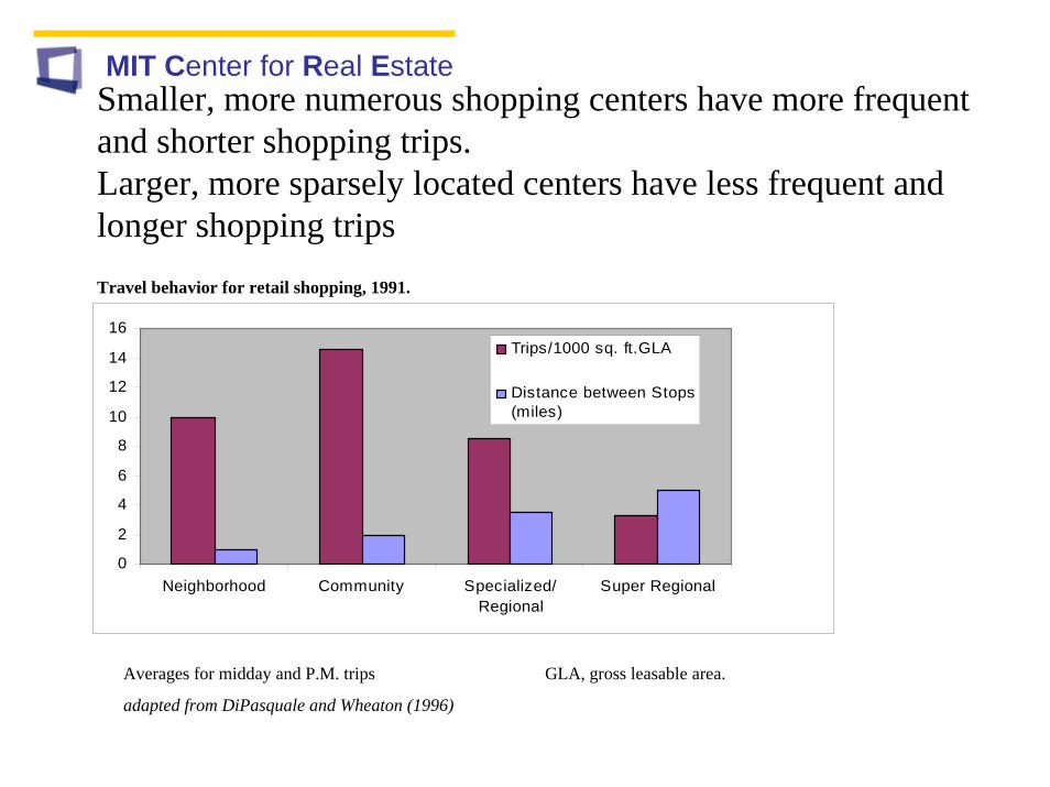
MIT Center for Real EstateSmaller, more numerous shopping centers have more frequent and shorter shopping trips.Larger, more sparsely located centers have less frequent and longer shopping tripsTravel behavior for retail shopping, 1991.

Averages for midday and P.M. trips GLA, gross leasable area.


0

2

4

6

8

10

12

14

16

Neighborhood Community Specialized/Regional

Super Regional

Trips/1000 sq. ft.GLA

Distance between Stops(miles)


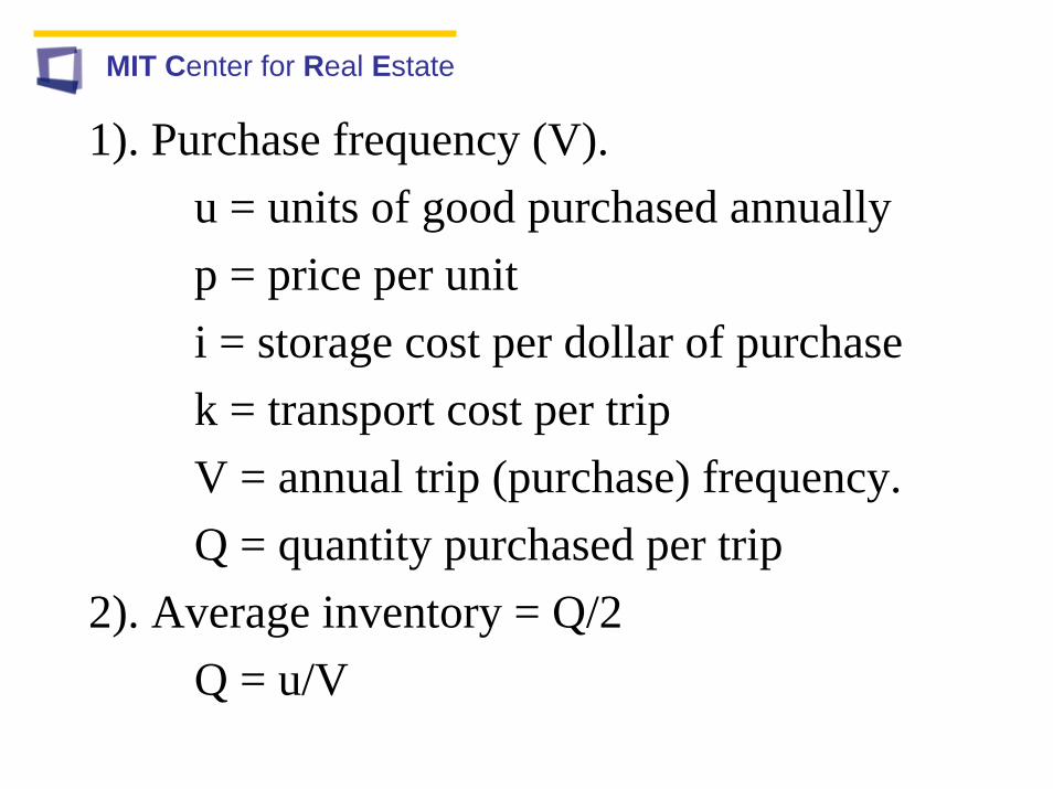
1). Purchase frequency (V). u = units of good purchased annuallyp = price per uniti = storage cost per dollar of purchasek = transport cost per tripV = annual trip (purchase) frequency.Q = quantity purchased per trip

2). Average inventory = Q/2Q = u/V


3). Annual consumption costs (CC):CC = pu + kV +i[pu/2V]

4). Minimizing with respect to V:implies ∂CC/ ∂V = k – ipu/2V2 = 0or: V* = [ipu/2k]1/2

5). How do V* (and Q) vary with i, u, k?


Classical Retail Market Areas when retailers compete over only price and consumers shop where the full price (including travel cost is lowest).

Location

Consumer’s full price

P P0P0

P + kT

TT

DD

MIT Center for eal stateR E6). Market areas and imperfect competition.

v = frequency of purchase trips (good consumption)f = density of buyers along linemc = wholesale price or marginal cost of goods to retailer. c = fixed cost of retailers (structure…)P = retail price of good.D = distance between stores [even spacing?]T = market area size (one side distance)S = retailer sales


7). Market areas based on equal purchase costs: P + kT = P0 + k(D-T) impliesT = [P0 – P + kD]/2kS = 2vTf = vf[P0 – P + kD]/k

8). Profit maximization (with respect to P given P0):π = [P – mc]S - c∂ π/∂ P = S + ∂ S/∂P [P-mc] = 0 implies:

P = [P0 + kD + mc]/2


9). Nash (“A Beautiful Mind”) Equilibrium assumption: P0 = P implies:

P = kD + mc, T = D/2, S = Dvf[profits higher with less competition, why?]

10). Free entry determines store density (1/D) so as to erode profit:

π = [P – mc]Dvf – c = 0 implies:P = mc + c/Dvf


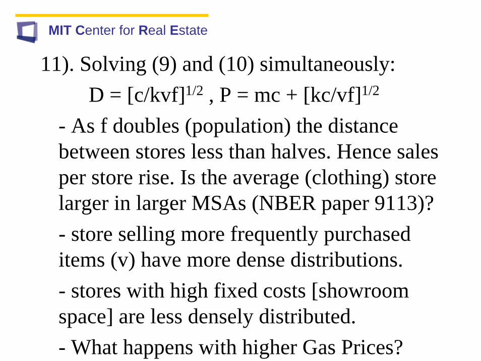
11). Solving (9) and (10) simultaneously:D = [c/kvf]1/2 , P = mc + [kc/vf]1/2

- As f doubles (population) the distance between stores less than halves. Hence sales per store rise. Is the average (clothing) store larger in larger MSAs (NBER paper 9113)?- store selling more frequently purchased items (v) have more dense distributions.- stores with high fixed costs [showroom space] are less densely distributed. - What happens with higher Gas Prices?

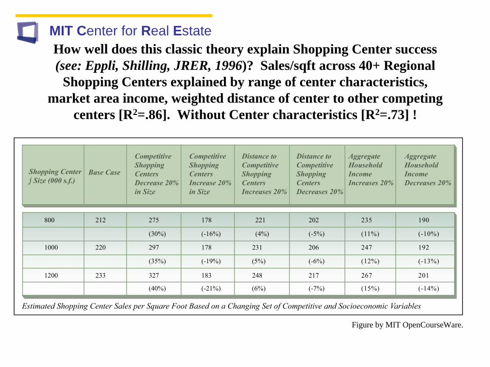
MIT Center for Real EstateHow well does this classic theory explain Shopping Center success (see: Eppli, Shilling, JRER, 1996)? Sales/sqft across 40+ Regional

Shopping Centers explained by range of center characteristics, market area income, weighted distance of center to other competing

centers [R2=.86]. Without Center characteristics [R2=.73] !

Shopping Centerj Size (000 s.f.)

Base Case

Competitive Shopping Centers Increase 20% in Size

Distance to Competitive Shopping Centers Increases 20%

Distance to Competitive Shopping Centers Decreases 20%

Aggregate Household IncomeIncreases 20%

Aggregate Household IncomeDecreases 20%

Competitive Shopping Centers Decrease 20% in Size

Estimated Shopping Center Sales per Square Foot Based on a Changing Set of Competitive and Socioeconomic Variables

212

220

233

800

1000

1200

275

(30%)

297

(35%)

327

(40%)

178

(-16%)

178

(-19%)

183

(-21%)

221

(4%)

231

(5%)

248

(6%)

202

(-5%)

206

(-6%)

217

(-7%)

235

(11%)

247

(12%)

267

(15%)

190

(-10%)

192

(-13%)

201

(-14%)

Figure by MIT OpenCourseWare.

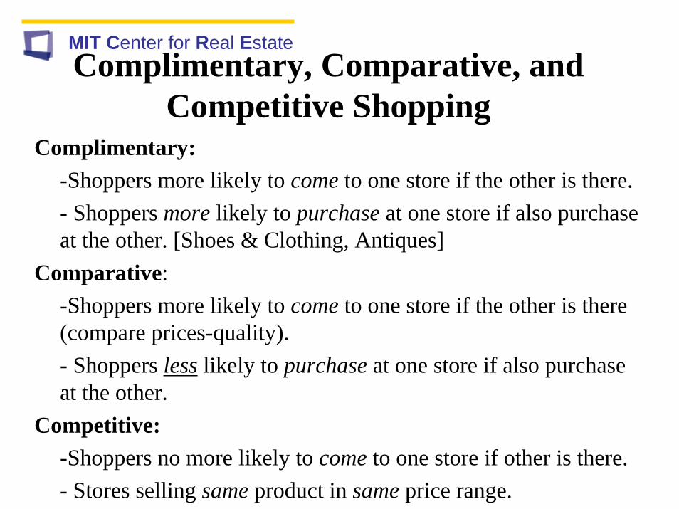
MIT Center for Real EstateComplimentary, Comparative, and

Competitive Shopping Complimentary:

-Shoppers more likely to come to one store if the other is there. - Shoppers more likely to purchase at one store if also purchase at the other. [Shoes & Clothing, Antiques]

Comparative: -Shoppers more likely to come to one store if the other is there (compare prices-quality). - Shoppers less likely to purchase at one store if also purchase at the other.

Competitive:-Shoppers no more likely to come to one store if other is there. - Stores selling same product in same price range.


Complimentary – Comparison Shopping Synergyv: # visits to each store if in and isolated location n: number of stores in “cluster” or centers: # visits to each store in cluster = total cluster visits x probability of store visit given visit to cluster. Total cluster visits = vn α

α: attraction factor for “clustering” [> 0] Probability of store visit if at cluster = 1/n β

β: degree stores compliment/compete [=0 if pure compliments, =1 if pure competitors] Hence: s = vn(α- β), and stores cluster if (α- β ) > 0

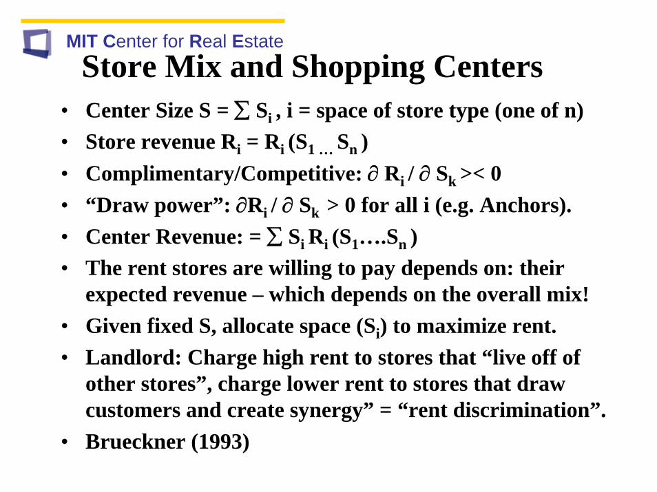
MIT Center for Real EstateStore Mix and Shopping Centers

• Center Size S = ∑ Si , i = space of store type (one of n)• Store revenue Ri = Ri (S1 … Sn ) • Complimentary/Competitive: ∂ Ri / ∂ Sk >< 0 • “Draw power”: ∂Ri / ∂ Sk > 0 for all i (e.g. Anchors). • Center Revenue: = ∑ Si Ri (S1….Sn )• The rent stores are willing to pay depends on: their

expected revenue – which depends on the overall mix!• Given fixed S, allocate space (Si) to maximize rent.• Landlord: Charge high rent to stores that “live off of

other stores”, charge lower rent to stores that draw customers and create synergy” = “rent discrimination”.

• Brueckner (1993)

MIT Center for Real EstateT a b le 1 : A v erag e leas e te rm s b y ty p e o f s to

Average Shopping

Center Lease terms by store

category1. Anchor2.Access

3. Apparel Unixex4. Children

5. Women specialty6. Women7. Mens8. Shoes

9. Jewelry10. Misc.

11. Discount12. Drug13. Books

14. Services17. Hobby18. Audio

20. Theatre21. Restaurant

re .

S to rec ate g ory

UL Ia re a11

S a mplea re a

UL I% 22

S a mple %

U LI R e nt33

S a mplere nt

UL I S ale s 44

1 10 2 .9 1 26 .4 1.0 1 .4 7 2.1 8 2.3 6 1 48 .1

2 .8 .7 7.9 8.3 33 .5 72 .1 2 78 .4

3 2.7 5.5 6.0 5.8 20 .3 36 .8 2 61 .2

4 2.1 3.3 5.0 5.4 21 .0 35 .5 2 68 .9

5 2.6 3.7 5.1 5.9 20 .1 36 .9 2 35 .4

6 3.9 5.9 5.0 5.3 15 .0 28 .9 1 75 .6

7 2.3 2.5 6.0 6.0 16 .2 36 .2 2 03 .9

8 2.2 2.4 6.0 6.2 18 .8 37 .3 2 32 .5

9 1.1 1.3 6.0 6.6 40 .5 82 .1 5 25 .4

1 0 1.8 2.3 5.6 5.7 18 .7 42 .8 2 31 .1

1 1 42 .6 29 .7 2.5 2.4 3.5 13 .2 1 29 .3

1 2 8.0 6.4 3.7 3.2 8.6 19 .3 2 10 .8

1 3 2.9 2.9 6.0 7.4 17 .3 40 .4 2 07 .2

1 4 1.3 2.3 4.7 6.1 19 .1 39 .7 2 37 .8

1 5 1.8 3.0 6.2 6.3 24 .2 36 .1 2 66 .1

1 7 3.9 4.1 5.5 6.0 13 .8 31 .0 1 91 .2

1 8 2.4 2.5 4.7 5.8 19 .6 42 .3 2 90 .3

2 0 8.9 5.6 8.9 17 .1 13 .7 40 .9 93 .4

2 1 5.6 4.1 5.0 6.5 12 .8 40 .5 2 25 .4

2 2

2 3

.9

.8

.9

.7

7.9

7.8

8.7

8.9

32 .2

39 .5

74 .2

1 12 .3

3 05 .1

3 36 .2

1. G ro ss leas ed a rea p e r s t ore , 1 00 0 s of s q u are fee t. 2 . P ercen t age o f gro s s s a le s p a id a s


Retail Rent: Percentage plus Base

Rental payments = R + max[0, r(S - B)]

R = Flat rent per square foot.r = Percentage of sales to be made as a rental payment.S = Sales per square foot.B = Threshold sales per square foot, or breakpoint.

Retail lease income as a function of store sales

Lease Income $/sqft

Base rent (R)

Percentage Rent (rS)

Sales $/sqft (S)

Figure by MIT OpenCourseWare.


Explanation for Percentage Rent• Risk Sharing: tenant pays fixed rent, absorbs

business risk if landlord more risk adverse. If both equally risk adverse =% rent [why only retail?].

• Not a substitute for fixed rent [notice that tenants paying higher fixed tend to pay higher % as well]

• With fixed rent, landlord can relet space to the detriment of existing tenants – and face no consequences until their leases renew.

• With percentage rent, landlord faces immediate loss in rental revenue if his actions in any way hurt the sales of existing tenants [Wheaton]


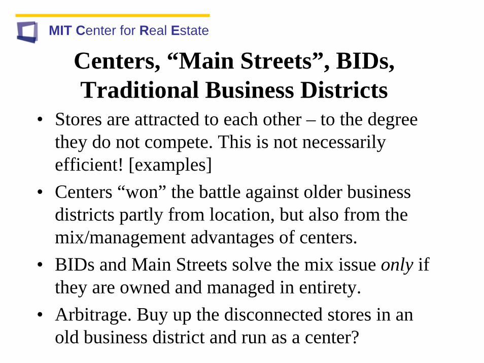
Centers, “Main Streets”, BIDs, Traditional Business Districts

• Stores are attracted to each other – to the degree they do not compete. This is not necessarily efficient! [examples]

• Centers “won” the battle against older business districts partly from location, but also from the mix/management advantages of centers.

• BIDs and Main Streets solve the mix issue only if they are owned and managed in entirety.

• Arbitrage. Buy up the disconnected stores in an old business district and run as a center?


Retail Market Analysis –done Right

Predicting Shopper patronage at 13 major retail centers and regional malls in the Boston Market

Map of Boston metropolitan area removed due to copyright restrictions.

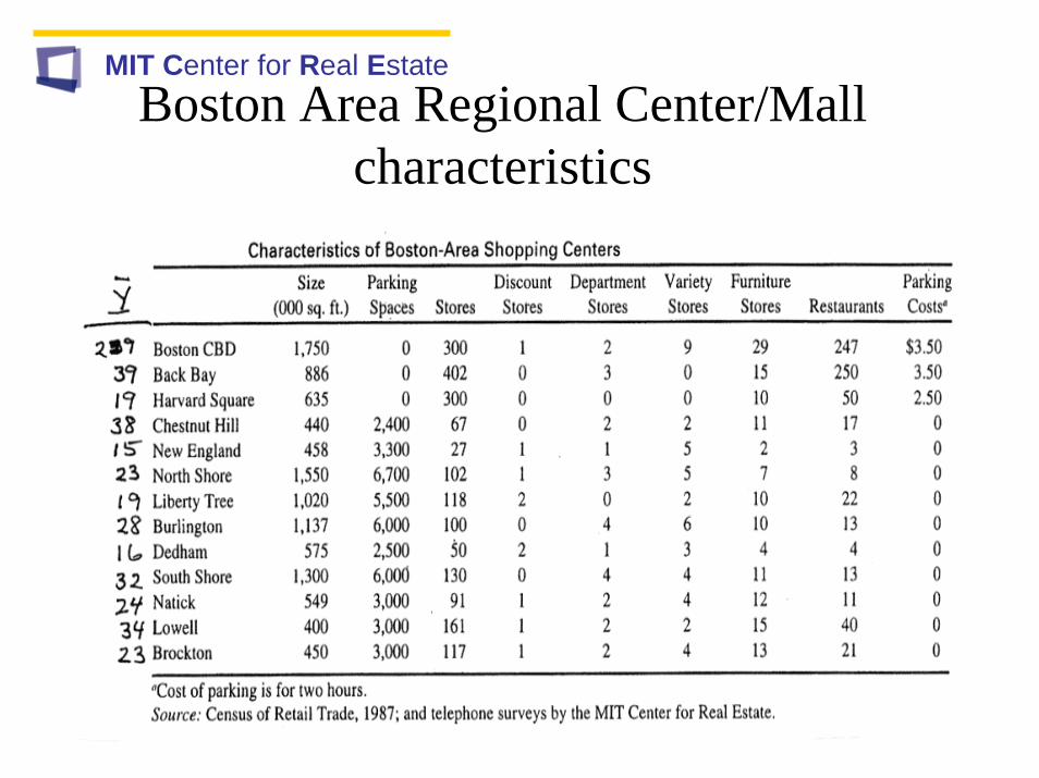
MIT Center for Real EstateBoston Area Regional Center/Mall

characteristics


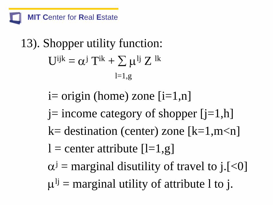
13). Shopper utility function:Uijk = αj Tik + ∑ μlj Z lk

l=1,g

i= origin (home) zone [i=1,n]j= income category of shopper [j=1,h]k= destination (center) zone [k=1,m<n]l = center attribute [l=1,g]αj = marginal disutility of travel to j.[<0]μlj = marginal utility of attribute l to j.


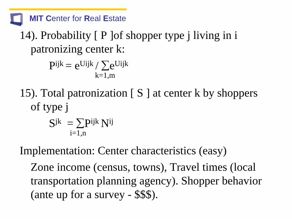
14). Probability [ P ]of shopper type j living in i patronizing center k:

Pijk = eUijk / ∑eUijkk=1,m

15). Total patronization [ S ] at center k by shoppers of type j

Sjk = ∑Pijk Niji=1,n

Implementation: Center characteristics (easy) Zone income (census, towns), Travel times (local transportation planning agency). Shopper behavior (ante up for a survey - $$$).


16). Estimation of utility parameters from actual Shopper patronization [ S ]:

ln(Sij1/Sijk) = αj (Ti1- Tik) + ∑μlj (Z l1- Z lk)l=1,g

Estimated over i,k (n x m-1 observations) for each shopper type j (h separate equations- one for each income group j).


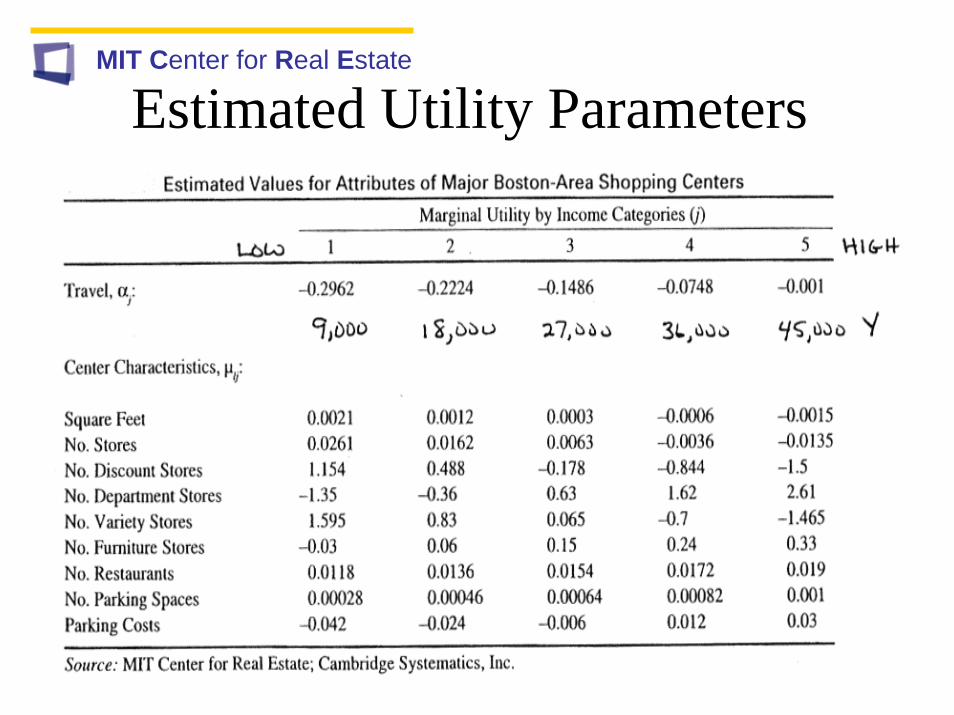
Estimated Utility Parameters


Predicted Shopping Center Patronage


How will the Retail system respond to higher Gasoline Prices?

• People want to shop “more locally”.• Less “cross hauling” – driving to other than the

nearest center.• Centers located near population masses do well,

those remotely located suffer. • Neighborhood and Community Center Sales

expand. • Stores previously locating in larger centers and

catering to lower income consumers now willing to increase outlets and locate more locally.

11.433j / 15.021j real estate economics - mit … · 5961 catalog and mail-order houses 148 558,813...

Documents