10.1 simvoi overview - treeplan chapter 10 monte carlo simulation using simvoi 10.4 random number...

Monte Carlo Simulation Using SimVoi 10

10.1 SIMVOI OVERVIEW SimVoi is a Monte Carlo simulation add-in for Microsoft Excel 2007 & 2010 & 2013 & 2016 (Windows) and Microsoft Excel 2011 & 2016 (Macintosh).

SimVoi facilitates Monte Carlo simulation by providing: Seventeen random number generator functions Ability to set the seed for random number generation Automatic repeated sampling for simulation Frequency distributions of simulation results Histogram, cumulative, and bivariate charts Value of information for input assumptions of your model

Your spreadsheet model may include uncontrollable uncertainties as input assumptions. Examples are demand for a new product, uncertain variable cost of production, or competitor reaction. You can use simulation to determine the uncertainty associated with the model's output (annual profit). You assess the probabilities for the input assumptions, and SimVoi automates the simulation by trying hundreds or thousands of what-ifs consistent with your assessments.

SimVoi provides (1) random number generator functions as inputs for your model, (2) automates Monte Carlo simulation, (3) summarizes results in tables and charts, and (4) computes value of information.

To use SimVoi:

(1) Refer to the “How To Install Addin” PDF file for installation instructions.

(2) Create a spreadsheet model.

(3) Optionally use SensIt to identify critical inputs.

(4) In each input cell of your model enter one of SimVoi's random number generator functions.

(5) In Windows Excel 2007 & 2010 & 2013 & 2016, choose Add-Ins > SimVoi Simulation (Control+Shift+V). In Mac Excel 2011, choose Tools > SimVoi Simulation (Option+Command+v). In Mac Excel 2016, press Option+Command+v.

(6) Specify the model output cell, information cells, and the number of what-if trials.

(7) Interpret simulation results. SimVoi gives you tables, histograms, cumulative charts, bivariate charts, and value of information.

110 Chapter 10 Monte Carlo Simulation Using SimVoi

All of SimVoi’s functionality is in the single SimVoi XLAM file. There is no separate setup file or help file. When you use SimVoi on a Windows computer, it does not create any Windows Registry entries (although Excel may use such entries to keep track of its add-ins).

10.2 USING SIMVOI FUNCTIONS SimVoi adds seventeen random number generator functions to Excel:

RandBeta(alpha,beta,,[MinValue],[MaxValue])

RandBinomial(trials,probability_s)

RandBiVarNormal(mean1,stdev1,mean2,stdev2,correl12)

RandCumulative(value_cumulative_table)

RandDiscrete(value_discrete_table)

RandExponential(lambda)

RandInteger(bottom,top)

RandLogNormal(Mean,StDev)

RandNormal(mean,standard_dev)

RandPoisson(mean)

RandSample(population)

RandTriangular(minimum,most_likely,maximum)

RandTriBeta(minimum,most_likely,maximum,[shape])

RandTruncBiVarNormal(mean1,stdev1,mean2,stdev2,correl12, [min1],[max1],[min2],[max2])

RandTruncLogNormal(Mean,StDev,[MinValue],[MaxValue])

RandTruncNormal(Mean,StDev,[MinValue],[MaxValue])

RandUniform(minimum,maximum)

You can use these functions as inputs to your model by typing in a worksheet cell. Or, in Windows Excel, from the Formulas ribbon, choose Insert Function and select the User Defined category. In Mac Excel, choose Formula Builder from the Formulas ribbon or choose Function from the Insert menu, search for Rand, and select from the User Defined list.

The SimVoi Rand functions include extensive error checking of arguments. After verifying that the functions are working properly, you can substitute the SimVoi Fast functions. These have minimal error checking and therefore run faster.

10.3 UPDATING LINKS TO SIMVOI FUNCTIONS When you insert a SimVoi random number generator function in a worksheet cell, the function is linked to the folder location of the current SimVoi XLAM file. During the current Excel session, the formula bar shows only the name of the SimVoi function. When you save and close the

wex=us

WyoSith

F

Mop

F

Ttoin

Iflo> Fim

workbook, Excexample, after c’C:\MyAddInsser defined fun

When you open ou deleted the imVoi XLAM

he saved path lo

igure 10.1 Exc

Mac Excel will pen or if SimV

igure 10.2 Exc

o update the lino the SimVoi Xn the Edit Link

f you do not imong as the SimV

Prepare > Editile > Info > Ed

menu choose Li

el saves the comclosing and reops\SimVoi-Addinctions like the

the workbookSimVoi XLAMfile is not loca

ocation. Excel

cel 2010 Warn

show a similarVoi has been ins

cel 2010 Edit L

nks, click the CXLAM file thats dialog box, c

mmediately updVoi XLAM filet Links to Files

dit Links to Filenks.

mplete path to pening the worin.xlam’!RandN ones containe

k, Excel looks fM file or if youated at the samdisplays a dial

ing To Update

r warning with stalled, click th

Links Dialog B

Change Sourcet is open. Selecclick the Close

date links whene is open or inss to see the diaes to see the Ed

10.3

the folder locarkbook, the forNormal(100,10d in the SimVo

for the SimVoiu opened the we path, Excel clog box like the

e Links

an Edit Links he Edit Links b

Box

e button. A filect the file usingbutton.

n the file is opestalled. To do s

alog box showndit Links dialog

3 Updating Links

ation of the Simrmula bar migh0). This is stanoi XLAM file.

i XLAM file usworkbook on ancannot find the e one shown b

button. If the Sbutton.

e browser windg the file brows

ened, you can uso, in Excel 20n below. In Excg box. In Mac

s To SimVoi Fun

mVoi function.ht show

ndard behavior

sing the saved nother compute SimVoi XLAMelow.

SimVoi XLAM

dow will open. ser, and click O

update the link007, choose Ofcel 2010 & 20Excel, from th

nctions 111

For

for Excel

path. If er where the M file at

M file is

Navigate OK. Back

ks later as ffice Button 13, choose he Edit


10.4 RANDOM NUMBER SEED The "Random Number Seed" edit box on the SimVoi dialog box allows you to set the seed for SimVoi's random number generator functions. The seed must be an integer in the range 1 through 2,147,483,647. SimVoi's random number generator functions are completely independent of Excel's built-in RAND function.

Random numbers generated by the computer are actually pseudo-random. The numbers appear to be random, and they pass various statistical tests for randomness. But they are actually calculated by an algorithm where each random number depends on the previous random number. Such an algorithm generates a repeatable sequence. The seed specifies where the algorithm starts in the sequence.

A Monte Carlo simulation model usually has uncontrollable inputs (uncertain quantities using random number generator functions), controllable inputs (decision variables that have fixed values for a particular set of simulation iterations), and an output variable (a performance measure or operating characteristic of the system).

One use of the random number seed is to reduce variation. For example, a simple queuing system model may have an uncertain arrival pattern, a controllable number of servers, and total cost (waiting time plus server cost) as output. To evaluate a different number of servers, specify the same seed before generating the uncertain arrivals. The variation in total cost will depend primarily on the different number of servers, not on the particular sequence of random numbers that generates the arrivals.

10.5 EXAMPLE MODEL In this example the analyst is interested in the uncertainty about cash flow for a software development project. It is difficult to express the uncertainty about cash flow directly, so the analyst has constructed a simple what-if spreadsheet model where the cash flow depends on assumptions about demand and costs. This analysis is based on a fixed price, but the other model inputs are uncertain.

Figure 10.3 Display of Example Model

To show the use of several random number generator functions, we use the truncated normal, triangular density, and a discrete distribution. In your own initial analysis of a problem, you might choose to use the triangular density with estimates of the minimum, most likely, and maximum values for each input assumption.

1

2

3

4

5

6

7

8

9

10

11

A B C D E F G H I

Software Decision Analysis

Controllable Input Variable

Unit Price $79

Uncertain Input Variables

Units Sold 898 Truncated Normal Mean=1000, StDev=200, Min=500, Max=1500

Unit Variable Cost $8.36 Triangular Min=$6, Mode=$8, Max=$11

Fixed Costs $12,000 Discrete Value Probability

Output Variable $10,000 0.3

Net Cash Flow $51,435 $12,000 0.5

$15,000 0.2

F

Afuin=

1ACSiprbo

F

Th

Sem

1

igure 10.4 For

After entering raunctions and thn Windows Exc

key repeatedly

0.6 MONAfter you specif

arlo simulationimulation or prress Option+Coox appears.

igure 10.5 Sim

he example mo

elect the Outpumust contain a f

3

4

5

6

7

8

9

10

A

Controllable In

Un

Uncertain Inp

Un

Un

Fix

Output Variab

Ne

rmulas of Exam

andom numberhe output functicel press F9 repy.

TE CARLfy random numn in Windows Eress Control+Sommand+v. In

mVoi Dialog B

odel is in a wor

ut Value Cell eformula that de

B

nput Variable

nit Price

ut Variables

nits Sold

nit Variable Cost

xed Costs

ble

et Cash Flow

mple Model

r generator funion Net Cash Fpeatedly. In M

LO SIMULmber generator

Excel 2007 & Shift+V. In Man Mac Excel 20

ox for Exampl

rksheet named

edit box, and poepends (usually

$79

=randtruncnor

=randtriangula

=randdiscrete(

=C6*(C4‐C7)‐C8

nctions, recalcuFlow are genera

Mac Excel, hold

LATION functions as in2010 & 2013 &c Excel 2011,

016, press Opti

le Simulation

d Model.

oint to a singley indirectly) on

C

mal(1000,200,500

r(6,8,11)

F9:G11)

8

10.6 M

ulate the worksating appropria

d down the Com

nputs to the mo& 2016, chooschoose Tools >ion+Command

e cell on your wn the model inp

0,1500)

Monte Carlo Simu

sheet to verify tate values. To mmand key and

odel, to performse Add-Ins > Si> SimVoi Simud+v. The SimV

worksheet. Theputs determined

ulation 113

that the recalculate, d press the

m Monte imVoi ulation or

Voi dialog

e output cell d by the


random number generator functions. In the example, the Output Value Cell is C10 on the Model worksheet, so the edit box displays Model!$C$10.

Information Cells are any other cells that you want to monitor for simulation results. In the example, the range C6:C8 is selected. All Information Cells must be on a single worksheet, which may be different from the worksheet containing the Output Value Cell. To select multiple cells or multiple ranges, select the first cell or contiguous range of cells, and then hold down the Ctrl key (Windows) or Command key (Macintosh) while you select the other cells or ranges of cells.

Click the Monte Carlo Simulation Only option button, select the Number of Trials edit box, and type an integer value for the number of what-if trials. This value, sometimes called the sample size or number of iterations, specifies the number of times the worksheet will be recalculated to determine output values of your model. One row is needed for each trial, and several additional rows are used for labels, so the number of trials is limited to approximately 65 thousand in XLS workbooks and slightly more than one million in XLSX workbooks. In the example, the Number of Trials is 500.

If you specify one or more Information Cells, you can check the Bivariate Charts box to obtain correlations and charts. The correlations are based on the total Number of Trials, but you may specify a smaller Number of Points for Each Bivariate Chart if you think the scatter pattern may be obscured by a large number of points. In the example, the Number of Points for Each Bivariate Chart is 100.

If you want a cumulative relative frequency chart in addition to a histogram for each variable, check the Cumulative Charts box, and specify the Number of Points for Each Cumulative Chart. In the example, the number of points is 100.

Leave the Random Number Seed unchanged, or select the Random Number Seed edit box, and type a number between 1 and 2,147,483,647. Use an integer value without commas or other separators. In the example, the seed is 12345678.

For terse help, click the Help button. SimVoi will create a help worksheet in your current workbook.

To start the simulation, click the Simulate button. Be sure to wait until all calculations and charts are complete.

10.7 SIMULATION DATA SimVoi creates a new worksheet in your Excel workbook named SimVoi.1 Simulation Data. Column A shows an integer for each trial 1 through the Number of Trials you specified. Column B shows the result in the Output Value Cell, and subsequent columns show results for each Information Cell.

SimVoi looks for text labels one or two cells to the left and one or two cells above the Output Value Cell and each Information Cell. If text is found, the text is shown in row 1; otherwise, the cell address is shown.

10.7 Simulation Data 115

Figure 10.6 First Ten Trials of Simulation Data

In columns to the right of the simulation results, SimVoi also displays the date, time, workbook name, and other information about the simulation.

Figure 10.7 SimVoi Summary Information on Simulation Data Sheet

1

2

3

4

5

6

7

8

9

10

11

A B C D E

Trial Net Cash Flow Units Sold Unit Variable Cost Fixed Costs

1 $48,155 854 $8.58 $12,000

2 $70,683 1170 $8.32 $12,000

3 $86,437 1371 $7.20 $12,000

4 $66,834 1079 $7.81 $10,000

5 $77,635 1283 $9.13 $12,000

6 $61,920 1060 $6.41 $15,000

7 $70,156 1125 $7.72 $10,000

8 $90,185 1422 $8.56 $10,000

9 $47,412 805 $7.72 $10,000

10 $47,154 835 $8.13 $12,000

1

2

3

4

5

6

7

8

9

10

11

12

13

14

15

16

17

18

19

20

21

22

23

24

25

G H I

SimVoi Simulation Data

Date (current date)

Time (current time)

Workbook (file name)

Number of Trials 500

Seed 12345678

Output Value Worksheet Model

Output Value Cell $C$10

Output Value Label Net Cash Flow

Information Worksheet Model

Information Cell $C$6

Information Label Units Sold



Information Label Unit Variable Cost



Information Label Fixed Costs


10.8 UNIVARIATE SUMMARY SimVoi displays the Univariate Summary sheet for each simulation, regardless of which options are selected in the SimVoi dialog box. The top left of the sheet shows summary measures for the output variable and each of the information variables. The summary measures are based on Excel worksheet functions AVERAGE, STDEV, QUARTILE, and SKEW.

Figure 10.8 SimVoi Numerical Output for One-Output Example

Below the summary measures are selected percentiles, based on Excel’s PERCENTILE worksheet function. The QUARTILE and PERCENTILE functions both use interpolation when necessary, so some values may be fractional, e.g., the first quartile or twenty fifth percentile in this example. Refer to Excel's online help for the interpolation method used by the PERCENTILE function.

Figure 10.9 Portion of Excel PERCENTILE Values

For each variable SimVoi provides a five-column summary with histogram. The top section has simulation information and summary measures.

1

2

3

4

5

6

7

8

9

10

11

12

13

A B C D E

SimVoi Univariate Summary

Net Cash Flow Units Sold Unit Variable Cost Fixed Costs

Mean $58,661 998 $8.24 $11,948

St. Dev. $13,662 191 $1.01 $1,746

Mean St. Error $611 9 $0.05 $78

Skewness +0.146 +0.160 +0.300 +0.606

Minimum $21,700 520 $6.15 $10,000

First Quartile $49,194 862 $7.49 $10,000

Median $58,210 995 $8.14 $12,000

Third Quartile $67,787 1125 $8.89 $12,000

Maximum $95,938 1485 $10.79 $15,000

16

17

18

19

20

21

22

23

24

25

26

A B C D E

Excel PERCENTILE


0.0% $21,700 520 $6.15 $10,000

0.5% $28,253 560 $6.28 $10,000

1.0% $28,448 585 $6.35 $10,000

2.5% $33,934 657 $6.50 $10,000

5.0% $36,675 701 $6.70 $10,000

10.0% $40,857 747 $6.98 $10,000

15.0% $43,876 805 $7.15 $10,000

20.0% $47,316 832 $7.36 $10,000

25.0% $49,194 862 $7.49 $10,000

10.8 Univariate Summary 117

Figure 10.10 Portion of Univariate Summary for Each Variable

In the five-column range, the histogram is a combination chart, using an Excel column chart type for the vertical bars and an XY Scatter chart type for the horizontal axis.

Figure 10.11 Histogram

The histogram is based on the numerical values of the frequency distribution located below the histogram and optional cumulative distribution chart. The distribution is computed using Excel’s array-entered FREQUENCY worksheet function.

1

2

3

4

5

6

7

8

9

10

H I J K L

SimVoi Univariate Summary Mean $58,661

Date (current date) St. Dev. $13,662

Time (current time) Mean St. Error $611

Trials 500 Skewness +0.146

Seed 12345678

Workbook (file name) Minimum $21,700

First Quartile $49,194

Worksheet Model Median $58,210

Cell $C$10 Third Quartile $67,787

Label Net Cash Flow Maximum $95,938

$20,000 $30,000 $40,000 $50,000 $60,000 $70,000 $80,000 $90,000 $100,000

0

10

20

30

40

50

60

70

80

Net Cash Flow, Column Width = $5,000

Column Frequen

cy

SimVoi Histogram For 500 Trials


Figure 10.12 Frequency Distribution

If the Cumulative Charts box is checked on the SimVoi dialog box, the chart of cumulative relative frequency is shown below the histogram.

Figure 10.13 Cumulative Chart

The cumulative chart is based on the sorted values and the cumulative relative frequencies, located in columns to the right of the charts for the variables.

49

50

51

52

53

54

55

56

57

58

59

60

61

62

63

64

65

66

H I

Upper Limit Frequency

$20,000 0

$25,000 1

$30,000 6

$35,000 8

$40,000 30

$45,000 38

$50,000 52

$55,000 74

$60,000 67

$65,000 64

$70,000 63

$75,000 33

$80,000 32

$85,000 14

$90,000 9

$95,000 8

$100,000 1

0.0

0.1

0.2

0.3

0.4

0.5

0.6

0.7

0.8

0.9

1.0

$20,000 $30,000 $40,000 $50,000 $60,000 $70,000 $80,000 $90,000 $100,000

Cumulative Relative Freq

uen

cy

Net Cash Flow

SimVoi Cumulative Chart For 100 Trials

10.9 Bivariate Summary 119

Figure 10.14 First Ten Values for Cumulative Charts

The cumulative relative frequencies start at 1/(2*N), where N is the number of trials, and increase by 1/N. The rationale is that the lowest ranked value of the sample values from the simulation is an estimate of the population values in the range from 0 to 1/N. The lowest ranked value is associated with the median of that range.

10.9 BIVARIATE SUMMARY If there are Information Cells and the Bivariate Charts box is checked in the SimVoi dialog box, SimVoi creates a Bivariate Summary sheet. The top left area displays correlation coefficients, r, and coefficients of determination, r-squared, for each pair of variables, based on Excel’s CORREL and RSQ worksheet functions.

Figure 10.15 Bivariate Numerical Results

1

2

3

4

5

6

7

8

9

10

11

AJ AK AL AM AN

Net Cash Flow Units Sold Unit Variable Cost Fixed Costs Cumul.Rel.Freq.

$26,634 539 $6.41 $10,000 0.005

$30,400 601 $6.60 $10,000 0.015

$30,782 614 $6.63 $10,000 0.025

$33,722 676 $6.63 $10,000 0.035

$36,397 696 $6.78 $10,000 0.045

$37,711 701 $6.87 $10,000 0.055

$38,326 717 $6.96 $10,000 0.065

$38,446 732 $6.98 $10,000 0.075

$39,518 743 $7.04 $10,000 0.085

$39,668 744 $7.05 $10,000 0.095

1

2

3

4

5

6

7

8

9

10

11

12

13

14

15

16

17

18

A B C D E

SimVoi Bivariate Summary

Correlation Coefficient, r

Excel CORREL, 500 Trials


Net Cash Flow 1.0000 0.9890 ‐0.0388 ‐0.1417

Units Sold 0.9890 1.0000 0.0342 ‐0.0145

Unit Variable Cost ‐0.0388 0.0342 1.0000 ‐0.0144

Fixed Costs ‐0.1417 ‐0.0145 ‐0.0144 1.0000

Coefficient of Determination, r‐squared

Excel RSQ, 500 Trials


Net Cash Flow 1.0000 0.9781 0.0015 0.0201

Units Sold 0.9781 1.0000 0.0012 0.0002

Unit Variable Cost 0.0015 0.0012 1.0000 0.0002

Fixed Costs 0.0201 0.0002 0.0002 1.0000


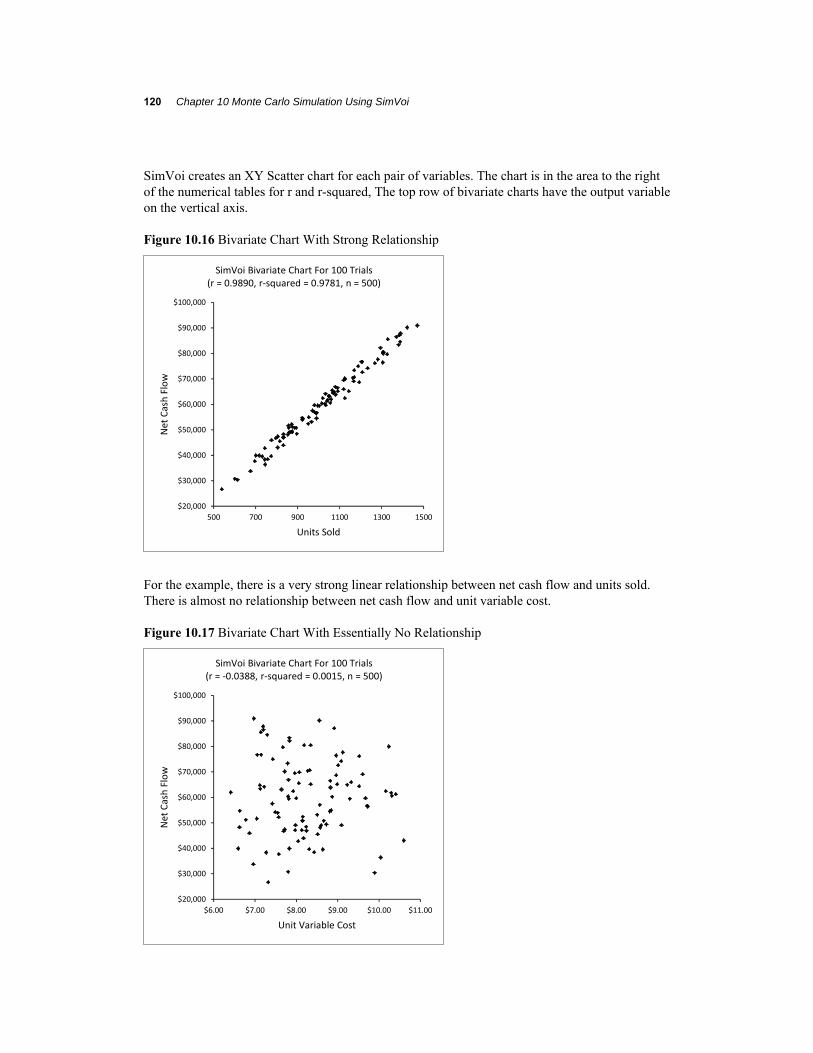
SimVoi creates an XY Scatter chart for each pair of variables. The chart is in the area to the right of the numerical tables for r and r-squared, The top row of bivariate charts have the output variable on the vertical axis.

Figure 10.16 Bivariate Chart With Strong Relationship

For the example, there is a very strong linear relationship between net cash flow and units sold. There is almost no relationship between net cash flow and unit variable cost.

Figure 10.17 Bivariate Chart With Essentially No Relationship

$20,000

$30,000

$40,000

$50,000

$60,000

$70,000

$80,000

$90,000

$100,000

500 700 900 1100 1300 1500

Net Cash Flow

Units Sold

SimVoi Bivariate Chart For 100 Trials(r = 0.9890, r‐squared = 0.9781, n = 500)

$20,000

$30,000

$40,000

$50,000

$60,000

$70,000

$80,000

$90,000

$100,000

$6.00 $7.00 $8.00 $9.00 $10.00 $11.00

Net Cash Flow

Unit Variable Cost

SimVoi Bivariate Chart For 100 Trials(r = ‐0.0388, r‐squared = 0.0015, n = 500)

10.10 Value of Information 121

Each bivariate chart is based on data arranged in columns located to the right of the charts.

Figure 10.18 First Ten Trials for Bivariate Charts

The top ten trials of data for the bivariate charts is the same as the top ten trials on the Simulation Data sheet. The entire Simulation Data sheet may be deleted without affecting the display of the bivariate charts.

10.10 VALUE OF INFORMATION Extending the Monte Carlo simulation example, the decision maker must decide between the software project and a fixed price job that would pay $50,000 using the same commitment of time and related resources. Before choosing, the decision maker could gather some information to help resolve the uncertainty associated with the software project. Which information about the three uncertainties is most valuable, and how much should the decision maker be willing to pay for the information?

The analyst uses SimVoi’s option for Value of Information to help answer the decision maker’s questions.

SimVoi is appropriate for this kind of analysis if the Output Value Cell is a monetary value and the Information Cells are uncertain inputs to the model.

The Number of Brackets box specifies the number of equally-probable ranges of values used to approximate the probability distributions for the value of information calculations.

The Trials per Bracket box specifies the number of trial used for approximating each of the brackets.

With 25 brackets and 20 trials per bracket, the simulation uses 25*20 = 500 trials. Using the same random number seed, 12345678, the simulation results will be the same as before. The histograms, cumulative charts, and bivariate charts will also be the same.

1

2

3

4

5

6

7

8

9

10

11

AP AQ AR AS


$48,155 854 $8.58 $12,000

$70,683 1170 $8.32 $12,000

$86,437 1371 $7.20 $12,000

$66,834 1079 $7.81 $10,000

$77,635 1283 $9.13 $12,000

$61,920 1060 $6.41 $15,000

$70,156 1125 $7.72 $10,000

$90,185 1422 $8.56 $10,000

$47,412 805 $7.72 $10,000

$47,154 835 $8.13 $12,000

12

F

Si

F

Thth

1

1

1

1

1

1

1

1

1

1

2

2

22 Chapter 10

igure 10.19 Si

imVoi creates

igure 10.20 Ch

he chart showshe value of an a

1

2

3

4

5

6

7

8

9

10

11

12

13

14

15

16

17

18

19

20

21

SimVoi Value

$0

$1,000

$2,000

$3,000

$4,000

$5,000

$6,000

$20,0

Value Of Inform

ation

0 Monte Carlo Sim

imVoi Dialog B

a chart showin

hart for Value

s how the valuealternative situ

A

Of Information

000 $30,000 $

U

mulation Using S

Box for Simula

ng the value of

of Information

e of informatioation.

B C

$40,000 $50,000

Valu

SimVoi Value

Units Sold Uni

SimVoi

ation and Valu

information fo

n for Each Info

on for the situat

C D

$60,000 $70,00

ue Of Alternative

e of Information

it Variable Cost

ue of Informatio

or each Inform

ormation Variab

tion described

E

00 $80,000 $9

Fixed Costs

on

ation Cell.

ble

by the model d

F G

90,000 $100,000

depends on

10.10 Value of Information 123

Referring to the Univariate Summary worksheet, the minimum value of simulation results for the software project is $21,700. If an alternative project has an outcome value less than $21,700, then clearly the software project is preferred, and there is no value for additional information about the three uncertain inputs of the software model.

Similarly, the maximum value of simulation results for the software project is $95,938. If an alternative project has an outcome value greater than $95,938, then clearly the alternative project is preferred, and there is no value for additional information about the three uncertain inputs of the software model.

If the alternative project has an outcome value between the two extremes of the software project, there may be some value of obtaining information about the uncertain assumptions used in the software model.

For the software example problem with an alternative project yielding $50,000, there is a positive value associated with information about Units Sold. There is zero value for information about Unit Variable Cost and Fixed Costs.

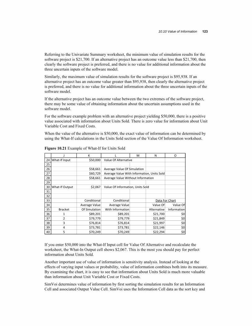
When the value of the alternative is $50,000, the exact value of information can be determined by using the What-If calculations in the Units Sold section of the Value Of Information worksheet.

Figure 10.21 Example of What-If for Units Sold

If you enter $50,000 into the What-If Input cell for Value Of Alternative and recalculate the worksheet, the What-In Output cell shows $2,067. This is the most you should pay for perfect information about Units Sold.

Another important use of value of information is sensitivity analysis. Instead of looking at the effects of varying input values or probability, value of information combines both into its measure. By examining the chart, it is easy to see that information about Units Sold is much more valuable than information about Unit Variable Cost or Fixed Costs.

SimVoi determines value of information by first sorting the simulation results for an Information Cell and associated Output Value Cell. SimVoi uses the Information Cell data as the sort key and

24

25

26

27

28

29

30

31

32

33

34

35

36

37

38

39

40

J K L M N O

What‐If Input $50,000 Value Of Alternative

$58,661 Average Value Of Simulation

$60,729 Average Value With Information, Units Sold

$58,661 Average Value Without Information

What‐If Output $2,067 Value Of Information, Units Sold

Conditional Conditional Data For Chart

Average Value Average Value Value Of Value Of

Bracket Of Simulation With Information Alternative Information

1 $89,201 $89,201 $21,700 $0

2 $79,779 $79,779 $21,849 $0

3 $76,814 $76,814 $21,997 $0

4 $73,781 $73,781 $22,146 $0

5 $70,249 $70,249 $22,294 $0


sorts from highest value down to lowest value. The Trial number is included to make it easy to verify the calculations.

Figure 10.22 Top Ten Rows of Sorted Data for Conditional EMV

Without any additional information, the average value of the simulation model is $58,661, i.e., the mean of Net Cash Flow shown on the Univariate Summary worksheet.

In this example, the Number of Brackets is 25 and the Trials per Bracket is 20. In the sorted data the first 20-row bracket is rows 5:24. When Units Sold is in the range 1349 to 1485, the associated Net Cash Flow values range from $83,313 to $95,938 with average value $89,201. SimVoi uses the name Conditional Average Value of Simulation for this average, and the value is displayed below the What-If area on the worksheet. If we know that Units Sold is in this high range, average value of the simulation is $89,201. The second bracket is rows 25:44 with conditional average value $79,779. And so on, down to the twenty-fifth bracket in rows 485:504 with conditional average value $31,784.

If we know that Units Sold is in a particular bracket, we compare the conditional average value of the simulation with the value of the alternative, and we choose the highest. The third column below the What-If area contains MAX functions, and the result is Conditional Average Value With Information.

The average of the Conditional Average Value With Information values is the Average Value With Information, Units Sold, shown in the What-If area. Also shown is the Average Value Without Information, i.e., the maximum of the Average Value Of Simulation and the Value Of Alternative. The Value of Information is the difference between the Average Value With Information and the Average Value Without Information.

When the value of the alternative is $50,000, the value of information is $2,067. The value of information is highest if the value of the alternative is the same as the average value of the simulation model, i.e., $64,139 – $58,661 = $5,478.

The data for the chart is computed using approximately 500 equally-spaced values between the minimum and maximum of the Net Cash Flow values from the simulation, including the value of Average Value Of Simulation.

3

4

5

6

7

8

9

10

11

12

13

14

AN AO AP

Sort Key

Trial Units Sold Net Cash Flow

322 1485 $90,700

43 1471 $90,922

188 1469 $92,973

239 1469 $93,967

206 1465 $91,794

236 1462 $95,938

114 1460 $93,300

320 1445 $92,665

136 1430 $88,405

8 1422 $90,185

10.11 Random Number Generator Functions 125

10.11 RANDOM NUMBER GENERATOR FUNCTIONS

RandBeta

Returns a random value from a beta distribution.

Syntax

RandBeta(alpha,beta,[minimum_value],[maximum_value])

The required arguments alpha and beta determine the shape of the probability density function and correspond to arguments of the same name used by the Excel family of beta functions. The optional arguments correspond to lower bound A and upper bound B in the Excel beta functions.

Remarks

If any argument is nonnumeric, RandBeta returns the #VALUE! error value.

If alpha <= 0 or beta <= 0, RandBeta returns the #NUM! error value.

If you omit values for minimum_value and maximum_value, RandBeta returns values with minimum_value = 0 and maximum_value = 1.

Example

The charts show the distribution for RandBeta with shape parameter values of 4 and 2, minimum_value 2 and maximum_value 10.

12

F

F

26 Chapter 10

igure 10.23 Ra

igure 10.24 Ra

0 Monte Carlo Sim

andBeta Exam

andBeta Exam

mulation Using S

mple Probability

mple Cumulativ

SimVoi

y Density Func

e Probability F

ction

Function


RandBinomial

Returns a random value from a binomial distribution. The binomial distribution can model a process with a fixed number of trials where the outcome of each trial is a success or failure, the trials are independent, and the probability of success is constant. RandBinomial counts the total number of successes for the specified number of trials. If n is the number of trials, the possible values for RandBinomial are the non-negative integers 0,1,...,n.

Syntax

RandBinomial(trials,probability_s)

Trials (often denoted n) is the number of independent trials.

Probability_s (often denoted p) is the probability of success on each trial.

Remarks

Returns #N/A if there are too few or too many arguments.

Returns #NAME! if an argument is text and the name is undefined.

Returns #NUM! if trials is non-integer or less than one, or probability_s is less than zero or more than one.

Returns #VALUE! if an argument is a defined name of a cell and the cell is blank or contains text.

Example

A salesperson makes ten unsolicited calls per day, where the probability of making a sale on each call is 70 percent. The uncertain total number of sales in one day is =RandBinomial(10,0.7)


Figure 10.25 RandBinomial Example Probability Mass Function

Figure 10.26 RandBinomial Example Cumulative Probability Function

Related Functions

FastBinomial: Same as RandBinomial without any error checking of the arguments.

CritBinom(trials,probability_s,RAND()): Excel's inverse of the cumulative binomial, or CritBinom(trials,probability_s,RandUniform(0,1)) to use the SimVoi Seed feature.

0.00

0.10

0.20

0.30

0 1 2 3 4 5 6 7 8 9 10

Total Number of Sales in 10 Calls, x

Pro

bab

ilit

y, P

(X=

x)

0.0

0.1

0.2

0.3

0.4

0.5

0.6

0.7

0.8

0.9

1.0

0 1 2 3 4 5 6 7 8 9 10

Total Number of Sales in 10 Calls, x

Cu

mu

lati

ve P

rob

abil

ity,

P(X

<=

x)


RandBiVarNormal

Returns two random values from a bivariate normal distribution with specified means, standard deviations, and correlation.

To use this random number generator function, select two adjacent cells on the worksheet. Type =RandBiVarNormal followed by numerical values for the five arguments or references to cells containing the values, separated by commas, enclosed in starting and ending parentheses. After typing the ending parentheses, do not press Enter. Instead, hold down the Control and Shift keys while you press Enter, thus "array entering" the function.

Syntax

RandBiVarNormal(mean1,stdev1,mean2,stdev2,correl12)

Remarks

Returns #REF! if the array function is not entered into two adjacent cells.

Returns #NUM! if a standard deviation is negative or the correlation is outside the range between -1 and +1.

Returns #VALUE! if an argument is not numeric.

Example

Select two adjacent cells, type

=RandBiVarNormal(100,10,50,5,0.5)

Hold down Control and Shift while you press Enter.

Related Function

FastBiVarNormal: Same as RandBiVarNormal without any error checking of the arguments. The two adjacent cells must be in the same row.


RandCumulative

Returns a random value from a piecewise-linear cumulative distribution. This function can model a continuous-valued uncertain quantity, X, by specifying points on its cumulative distribution. Each point is specified by a possible value, x, and a corresponding left-tail cumulative probability, P(X<=x). Random values are based on linear interpolation between the specified points.

Syntax

RandCumulative(value_cumulative_table)

Value_cumulative_table must be a reference, or the defined name of a reference, for a two-column range, with values in the left column and corresponding cumulative probabilities in the right column.

Remarks


Returns #NAME! if the argument is text and the name is undefined.

Returns #NUM! if the first (top) cumulative probability is not zero, if the last (bottom) cumulative probability is not one, or if the values or cumulative probabilities are not in ascending order.

Returns #REF! if the number of columns in the table reference is not two.

Returns #VALUE! if the argument is not a reference, if the argument is a defined name but not for a reference, or if any cell of the table contains text or is blank.

Example

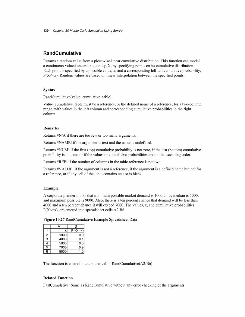
A corporate planner thinks that minimum possible market demand is 1000 units, median is 5000, and maximum possible is 9000. Also, there is a ten percent chance that demand will be less than 4000 and a ten percent chance it will exceed 7000. The values, x, and cumulative probabilities, P(X<=x), are entered into spreadsheet cells A2:B6.

Figure 10.27 RandCumulative Example Spreadsheet Data

The function is entered into another cell: =RandCumulative(A2:B6)

Related Function

FastCumulative: Same as RandCumulative without any error checking of the arguments.

123456

A Bx P(X<=x)

1000 0.04000 0.15000 0.57000 0.99000 1.0


Figure 10.28 RandCumulative Example Probability Density Function

Figure 10.29 RandCumulative Example Cumulative Probability Function

Market Demand, x, in units

Pro

babi

lity

Den

sity

, f(

x)

0

0.0001

0.0002

0.0003

0.0004

0.0005

0 2000 4000 6000 8000 10000

Market Demand, x, in units

Cu

mu

lativ

e P

rob

ab

ility

, P(X

<=

x

0

0.2

0.4

0.6

0.8

1

0 2000 4000 6000 8000 10000


RandDiscrete

Returns a random value from a discrete probability distribution. This function can model a discrete-valued uncertain quantity, X, by specifying its probability mass function. The function is specified by each possible discrete value, x, and its corresponding probability, P(X=x).

Syntax

RandDiscrete(value_discrete_table)

Value_discrete_table must be a reference, or the defined name of a reference, for a two-column range, with values in the left column and corresponding probability mass in the right column.

Remarks



Returns #NUM! if a probability is negative or if the probabilities do not sum to one.

Returns #REF! if the number of columns in the table reference is not two.

Returns #VALUE! if the argument is not a reference, if the argument is a defined name but not for a reference, or if any cell of the table contains text or is blank.

Example

A corporate planner thinks that uncertain market revenue, X, can be approximated by three possible values and their associated probabilities: P(X=10000) = 0.25, P(X=12000) = 0.50, and P(X=15000) = 0.25. The values and probabilities are entered into spreadsheet cells A2:B4.

Figure 10.30 RandDiscrete Example Spreadsheet Data

The function is entered into another cell: =RandDiscrete(A2:B4)

Related Function

FastDiscrete: Same as RandDiscrete without any error checking of the arguments.

1234

A Bx P(X=x)

$10,000 0.25$12,000 0.50$15,000 0.25


Figure 10.31 RandDiscrete Example Probability Mass Function

Figure 10.32 RandDiscrete Example Cumulative Probability Function

0.0

0.2

0.4

0.6

0.8

1.0

$8,000 $10,000 $12,000 $14,000 $16,000

Pro

ba

bili

ty M

ass

, P(X

=x)

Market Revenue, x

0.0

0.2

0.4

0.6

0.8

1.0

$8,000 $10,000 $12,000 $14,000 $16,000

Cu

mu

lativ

e P

roba

bilit

y, P

(X<

=x)

Market Revenue, x


RandExponential

Returns a random value from an exponential distribution. This function can model the uncertain time interval between successive arrivals at a queuing system or the uncertain time required to serve a customer.

Syntax

RandExponential(lambda)

Lambda is the mean number of occurrences per unit of time.

Remarks



Returns #NUM! if lambda is negative or zero.

Returns #VALUE! if the argument is a defined name of a cell and the cell is blank or contains text.

Examples

Cars arrive at a toll plaza with a mean rate of 3 cars per minute. The uncertain time between successive arrivals, measured in minutes, is =RandExponential(3). The average value returned by repeated recalculation of RandExponential(3) is 0.333.


Figure 10.33 RandExponential Example Probability Density Function

Figure 10.34 RandExponential Example Cumulative Probability Function

A bank teller requires an average of two minutes to serve a customer. The uncertain customer service time, measured in minutes, is =RandExponential(0.5). The average value returned by repeated recalculation of RandExponential(0.5) is 2.

Related Functions

FastExponential: Same as RandExponential without any error checking of the arguments.

LN(RAND())/lambda: Excel's inverse of the exponential, or LN(RandUniform(0,1))/lambda to use the SimVoi Seed feature.

RandPoisson: Counts number of occurrences for a Poisson process.

0

1

2

3

0 1 2 3

Tim e Betw een Successive Arrivals in M inutes, x

Pro

bab

ility

Den

sity

, f(x

)

0.0

0.1

0.2

0.3

0.4

0.5

0.6

0.7

0.8

0.9

1.0

0 1 2 3

Tim e Betw een Successive Arrivals in M inutes , x

Cu

mu

lati

ve P

rob

abili

ty, P

(X<=

x)


RandInteger

Returns a uniformly distributed random integer between two integers you specify.

Syntax

RandInteger(bottom,top)

Bottom is the smallest integer RandInteger will return.

Top is the largest integer RandInteger will return.

Remarks



Returns #NUM! if top is less than or equal to bottom.

Returns #VALUE! if bottom or top is not an integer or if an argument is a defined name of a cell and the cell is blank or contains text.

Example

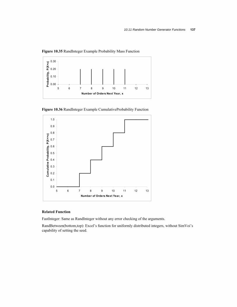
The number of orders a particular customer will place next year is between 7 and 11, with no number more likely than the others. The uncertain number of orders is =RandInteger(7,11).


Figure 10.35 RandInteger Example Probability Mass Function

Figure 10.36 RandInteger Example CumulativeProbability Function

Related Function

FastInteger: Same as RandInteger without any error checking of the arguments.

RandBetween(bottom,top): Excel’s function for uniformly distributed integers, without SimVoi’s capability of setting the seed.

0.00

0.10

0.20

0.30

5 6 7 8 9 10 11 12 13

Number of Orders Next Year, x

Pro

bab

ilit

y, P

(X=

x)

0.0

0.1

0.2

0.3

0.4

0.5

0.6

0.7

0.8

0.9

1.0

5 6 7 8 9 10 11 12 13

Number of Orders Next Year, x

Cu

mu

lati

ve P

rob

abil

ity,

P(X

<=

x)


RandLogNormal

Returns a random value from a lognormal distribution.

Syntax

RandLogNormal(mean,standard_dev)

RandNormal

Returns a random value from a normal distribution. This function can model a variety of phenomena where the values follow the familiar bell-shaped curve, and it has wide application in statistical quality control and statistical sampling.

Syntax

RandNormal(mean,standard_dev)

Mean is the arithmetic mean of the normal distribution.

Standard_dev is the standard deviation of the normal distribution.

Remarks



Returns #NUM! if standard_dev is negative.


Example

The total market for a product is approximately normally distributed with mean 60,000 units and standard deviation 5,000 units. The uncertain total market is =RandNormal(60000,5000).


Figure 10.37 RandNormal Example Probability Density Function

Figure 10.38 RandNormal Example Cumulative Probability Function

Related Function

FastNormal: Same as RandNormal without any error checking of the arguments.

NormInv(RAND(),mean,standard_dev): Excel's inverse of the normal, or NormInv(RandUniform(0,1),mean,standard_dev) to use the SimVoi Seed feature.

0.00000

0.00001

0.00002

0.00003

0.00004

0.00005

0.00006

0.00007

0.00008

0.00009

40000 45000 50000 55000 60000 65000 70000 75000 80000

Total Market Size , x

Pro

bab

ility

Den

sity

, f(x

)

0.0

0.1

0.2

0.3

0.4

0.5

0.6

0.7

0.8

0.9

1.0

40000 45000 50000 55000 60000 65000 70000 75000 80000

Total Market Size , x

Cu

mu

lati

ve P

rob

abili

ty, P

(X<=

x)


RandPoisson

Returns a random value from a Poisson distribution. This function can model the uncertain number of occurrences during a specified time interval, for example, the number of arrivals at a service facility during an hour. The possible values of RandPoisson are the non-negative integers, 0, 1, 2, ... .

Syntax

RandPoisson(mean)

Mean is the mean number of occurrences per unit of time.

Remarks



Returns #NUM! if mean is negative or zero.

Returns #VALUE! if mean is a defined name of a cell and the cell is blank or contains text.

Examples

Cars arrive at a toll plaza with a mean rate of 3 cars per minute. The uncertain number of arrivals in a minute is =RandPoisson(3). The average value returned by repeated recalculation of RandPoisson(3) is 3.


Figure 10.39 RandPoisson Example Probability Mass Function

Figure 10.40 RandPoisson Example CumulativeProbability Function

Example

A bank teller requires an average of two minutes to serve a customer. The uncertain number of customers served in a minute is =RandPoisson(0.5). The average value returned by repeated recalculation of RandPoisson(0.5) is 0.5.

Related Functions

FastPoisson: Same as RandPoisson without any error checking of the arguments.

RandExponential: Describes time between occurrences for a Poisson process.

0.00

0.10

0.20

0.30

0 1 2 3 4 5 6 7 8 9 10

Number of Arrivals in a Minute, x

Pro

bab

ilit

y, P

(X=

x)

0.0

0.1

0.2

0.3

0.4

0.5

0.6

0.7

0.8

0.9

1.0

0 1 2 3 4 5 6 7 8 9 10

Number of Arrivals in a Minute, x

Cu

mu

lati

ve P

rob

abil

ity,

P(X

<=

x)


RandSample

Returns a random sample without replacement from a population.

To use this random number generator function, select a number of cells equal to the sample size, either in a single column or in a single row. Type =RandSample( followed by a reference to the cells containing the population values, enclosed in parentheses. After typing the ending parentheses, do not press Enter. Instead, hold down the Control and Shift keys while you press Enter, thus "array entering" the function.

Syntax

RandSample(population)

The population argument is a reference to a range of values in a single column.

Remarks

Returns #N/A if the population range is not part of a single column.

Returns #REF! if the function is not entered into two adjacent cells.

Example

Type population values into cells A2:A6. For a sample of size 3, select cells B2:B4, and type =RandSample(A2:A6) but don't press Enter. Hold down Control and Shift while you press Enter. Press F9 to recalculate for a different sample.

Related Functions

FastColumnSample: Same as RandSample for two adjacent cells in the same column, without any error checking of arguments.

FastRowSample: Same as RandSample for two adjacent cells in the same row, without any error checking of arguments.

123456

A BPopulation Data Sample

29 7373 5713 294457


RandTriangular

Returns a random value from a triangular probability density function. This function can model an uncertain quantity where the most likely value (mode) has the largest probability of occurrence, the minimum and maximum possible values have essentially zero probability of occurrence, and the probability density function is linear between the minimum and the mode and between the mode and the maximum. This function can also model a ramp density function where the minimum equals the mode or the mode equals the maximum.

Syntax

RandTriangular(minimum,most_likely,maximum)

Minimum is the smallest value RandTriangular will return.

Most_likely is the most likely value RandTriangular will return.

Maximum is the largest value RandTriangular will return.

Remarks



Returns #NUM! if minimum is greater than or equal to maximum, if most_likely is less than minimum, or if most_likely is greater than maximum.


Example

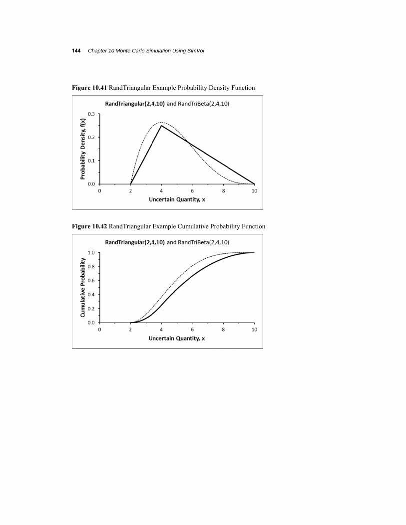
The minimum time required to complete a particular task that is part of a large project is 2 hours, the most likely time required is 4 hours, and the maximum time required is 10 hours.

The function returning the uncertain time required for the task is entered into a cell: =RandTriangular(4,6,10).

The probability density chart shows the difference between the RandTriangular function with its two linear segments and the smoother RandTriBeta function.

Related Function

FastTriangular: Same as RandTriangular without any error checking of arguments.

14

F

F

44 Chapter 10

igure 10.41 Ra

igure 10.42 Ra

0 Monte Carlo Sim

andTriangular

andTriangular

mulation Using S

Example Prob

Example Cum

SimVoi

bability Density

mulative Probab

y Function

bility Function


RandTriBeta

Returns a random value from a beta probability density function. This function can model an uncertain quantity where the most likely value (mode) has the largest probability of occurrence, and the minimum and maximum possible values have essentially zero probability of occurrence. The probability density function is a smooth curve between the minimum and the maximum with its highest point at the mode.

Syntax

RandTriBeta(minimum,most_likely,maximum,shape)

Minimum is the smallest value RandTriBeta will return.

Most_likely is the most likely value RandTriBeta will return.

Maximum is the largest value RandTriBeta will return.

Shape is an optional parameter which determines the peakedness of the density function. If a value for Shape is omitted, RandTriBeta uses the value Shape = 4.

Remarks



Returns #NUM! if minimum is greater than or equal to maximum, if most_likely is less than minimum, or if most_likely is greater than maximum.


Related Function

FastTriBeta: Same as RandTriBeta without any error checking of arguments.

Example

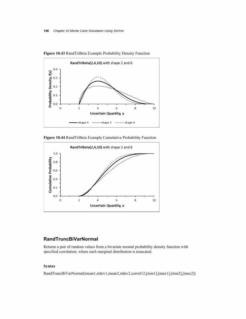
The minimum time required to complete a particular task that is part of a large project is 2 hours, the most likely time required is 4 hours, and the maximum time required is 10 hours.

The function returning the uncertain time required for the task is entered into a cell: = RandTriBeta (2,4,10).

The charts show the shapes of RandTriBeta(2,4,10) where the solid line uses the default shape value 4. The flatter dotted line shows RandTriBeta(2,4,10,2), and the peaked dashed line shows RandTriBeta(2,4,10,6).

14

F

F

R

Rsp

Sy

R

46 Chapter 10

igure 10.43 Ra

igure 10.44 Ra

RandTrunc

Returns a pair opecified correla

yntax

RandTruncBiVa

0 Monte Carlo Sim

andTriBeta Ex

andTriBeta Ex

BiVarNorm

f random valueation, where ea

arNormal(mean

mulation Using S

xample Probabi

xample Cumula

mal

es from a bivarach marginal di

n1,stdev1,mean

SimVoi

ility Density Fu

ative Probabilit

riate normal pristribution is tr

n2,stdev2,corr

unction

ty Function

robability densruncated.

rel12,[min1],[m

sity function wi

max1],[min2],[m

ith

max2])


RandTruncLogNormal

Returns a random value from a truncated log normal probability density function. This function can model an uncertain quantity with a positively-skewed density function where extreme values in the tails of the distribution are not desired. Subranges of the truncated UQ have the same relative probabilities as the same subranges of the original log normal distribution.

Syntax

RandTruncLogNormal(Mean,StDev,MinValue,MaxValue)

Mean and StDev are the parameters for the original log normal distribution.

MinValue is the smallest value RandTruncLogNormal will return.

MaxValue is the largest value RandTruncLogNormal will return.

MinValue and MaxValue are optional arguments.

Remarks: Same as RandTruncNormal

RandTruncNormal

Returns a random value from a truncated normal probability density function. This function can model an uncertain quantity with a bell-shaped density function where extreme values in the tails of the distribution are not desired. Subranges of the truncated UQ have the same relative probabilities as the same subranges of the original normal distribution.

Syntax

RandTruncNormal(Mean,StDev,MinValue,MaxValue)

Mean and StDev are the parameters for the original normal distribution.

MinValue is the smallest value RandTruncNormal will return.

MaxValue is the largest value RandTruncNormal will return.

MinValue and MaxValue are optional arguments.

Remarks

Returns #N/A if a value between MinValue and MaxValue is not found after 10,000 attempts.

Returns #NUM! if MinValue is greater than or equal to MaxValue.

Returns #VALUE! if an argument cannot be interpreted as a numeric value.


Related Function

FastTruncNormal: Same as RandTruncNormal, but with error checking only for maximum of 10,000 attempts.

Example

An uncertain quantity has a normal distribution with mean = 100 and standard deviation = 10, but values are restricted between 90 and 120.

The function returning the uncertain quantity is entered into a cell: = RandTruncNormal (100,10,90,120).

Figure 10.45 shows the original normal density function with mean = 100 and standard deviation = 10. The density function is rescaled so that the total area under the curve between 90 and 120 is equal to one. The corresponding cumulative distributions are shown in Figure 10.46.

For example, with the original normal density function, P(100<=X<=110) = 0.341, and P(110<=X<=120) = 0.136. The ratio of P(100<=X<=110) to P(110<=X<=120) is 0.341/0.136 = 2.512. Thus, a value in the range 100 to 110 is approximately 2.5 times as likely as a value in the range 110 to 120.

With the truncated normal density function, P(100<=X<=110) = 0.417, and P(110<=X<=120) = 0.166. The ratio of P(100<=X<=110) to P(110<=X<=120) is 0. 417/0.166 = 2.512. Thus, a value in the range 100 to 110 is still approximately 2.5 times as likely as a value in the range 110 to 120.


Figure 10.45 RandTruncNormal Probability Density Function

Figure 10.46 RandTruncNormal Cumulative Probability Function

RandUniform

Returns a uniformly distributed random value between two values you specify. As a special case, RandUniform(0,1) is the same as Excel's built-in RAND() function.

Syntax

RandUniform(minimum,maximum)

Minimum is the smallest value RandUniform will return.

Maximum is the largest value RandUniform will return.

Remarks


70 80 90 100 110 120 130

Value, x

Pro

ba

bili

ty D

en

sity

, f(

x)

0.0

0.2

0.4

0.6

0.8

1.0

70 80 90 100 110 120 130

Value, x

Cu

mul

ativ

e P

rob

ab

ility

, P

(X<

=x)



Returns #NUM! if minimum is greater than or equal to maximum.


Example

A corporate planner thinks that the company's product will garner between 10% and 15% of the total market, with all possible percentages equally likely in the specified range. The uncertain market proportion is =RandUniform(0.10,0.15).

Figure 10.47 RandUniform Example Probability Density Function

Figure 10.48 RandUniform Example Cumulative Probability Function

Related Function

FASTUNIFORM: Same as RandUniform without any error checking of the arguments.

0

10

20

30

0.08 0.09 0.10 0.11 0.12 0.13 0.14 0.15 0.16 0.17

Proportion of Total Market Captured, x

Pro

bab

ility

Den

sity

, f(x

)

0.0

0.1

0.2

0.3

0.4

0.5

0.6

0.7

0.8

0.9

1.0

0.08 0.09 0.10 0.11 0.12 0.13 0.14 0.15 0.16 0.17

Proportion of Total Market Captured, x

Cu

mu

lati

ve P

rob

abil

ity,

P(X

<=

x)

10.12 SimVoi Technical Details 151

10.12 SIMVOI TECHNICAL DETAILS SimVoi's random number generator functions are based on a uniformly distributed random number function called RandSeed which is not directly accessible by the user. RandSeed returns a random value x in the range 0<x<=1. Internally, decimal values for RandSeed are calculated by dividing a uniformly distributed random integer by 2,147,483,647, which is RandSeed's period. Random integers in the range 1 through 2,147,483,647 are generated using the well-documented Park-Miller algorithm, where each random integer depends on the previous random integer.

When SimVoi starts, the initial integer seed depends on the system clock. Unlike Excel's RAND() function, you can use SimVoi at any time to specify an integer seed in the range 1 through 2,147,483,647, which is used as the previous random integer for the sequence of random numbers generated by the SimVoi functions.

In the SimVoi dialog box, the Random Number Seed edit box changes the seed only for the SimVoi functions; it does not have any effect on Excel's built-in RAND() function.

Each of SimVoi's random number generator functions use RandSeed as a building block.

RandBeta(alpha,beta,,[MinValue],[MaxValue]) uses RandSeed as the cumulative probability in Excel's built-in BETAINV function.

RandBinomial(trials,probability_s) uses RandSeed as the cumulative probability in Excel's built-in CRITBINOM function.

RandBiVarNormal(mean1,stdev1,mean2,stdev2,correl12) uses two values of RandNormal to obtain correlated normal values.

RandCumulative(value_cumulative_table) uses the value of RandSeed, R, searches to find the adjacent cumulative probabilities that bracket R, and interpolates on the linear segment of the cumulative distribution to find the corresponding value.

RandDiscrete(value_discrete_table) compares RandSeed with summed probabilities of the input table until the sum exceeds the RandSeed value, and then returns the previous value from the input table.

RandExponential(lambda) uses the value of RandSeed, R, as follows. If the exponential density function is f(t) = lambda*EXP(-lambda*t), the cumulative is P(T<=t) = 1 - EXP(-lambda*t). Associating R with P(T<=t), the inverse cumulative is t = -LN(1-R)/lambda. Since R and 1-R are both uniformly distributed between 0 and 1, SimVoi uses -LN(R)/lambda for the returned value.

RandInteger(bottom,top) returns bottom + INT(RandSeed*(top-bottom+1)).

RandLogNormal(Mean,StDev) transforms Mean and StDev, uses RandSeed and the transformed values in SimVoi’s RandNormal function, and transforms the normal result to obtain the log normal value.

RandNormal(mean,standard_dev) uses two RandSeed values in the well-documented Box-Muller method.

RandPoisson(mean) compares RandSeed with cumulative probabilities of Excel's built-in POISSON function until the probability exceeds the RandSeed value, and then returns the previous value.


RandSample(population) uses RandSeed for each of the cells that were selected when the function was array-entered, avoiding population values that have already been selected, thus providing sampling without replacement.

RandTriangular(minimum,most_likely,maximum) uses RandSeed once. The triangular density function has two linear segments, so the cumulative distribution has two quadratic segments. The returned value is determined by interpolation on the appropriate quadratic segment.

RandTriBeta(minimum,most_likely,maximum,[shape]) uses several formulas to transform min-mode-max into the beta function alpha and beta parameters and then uses RandSeed as the cumulative probability in Excel's built-in BETAINV function.

RandTruncBiVarNormal(mean1,stdev1,mean2,stdev2,correl12,[min1],[max1],[min2], [max2]) uses values of RandBiVarNormal until normal values are found between the pairs of min and max values or until it has made 10,000 attempts.

RandTruncLogNormal(Mean,StDev,MinValue,MaxValue)) uses values of RandNormal until a log normal value is found between MinValue and MaxValue or until it has made 10,000 attempts.

RandTruncNormal(Mean,StDev,MinValue,MaxValue)) uses values of RandNormal until a value is found between MinValue and MaxValue or until it has made 10,000 attempts.

RandUniform(minimum,maximum) returns minimum + RandSeed*(maximum-minimum). RandUniform(0,1) is equivalent to Excel's built-in RAND() function.

SimVoi includes a Fast... version of each of the seventeen functions, e.g., FastBinomial, FastCumulative, etc. The Fast... functions are identical to the Rand... functions except there is no error checking of arguments.

10.1 simvoi overview - treeplan chapter 10 monte carlo simulation using simvoi 10.4 random number...

Documents