1

WELFARE ANALYSIS USING LOGSUM DIFFERENCES VS. RULE OF 1 HALF: A SERIES OF CASE STUDIES 2

3 Shuhong Ma 4

Associate Professor 5 School of Highways, Chang’an University 6

Xi’an, China, 710064 7 msh@chd.edu.cn 8

9 Kara M. Kockelman 10

Professor and William J. Murray Jr. Fellow 11 Department of Civil, Architectural and Environmental Engineering 12

The University of Texas at Austin 13 kkockelm@mail.utexas.edu 14

Phone: 512-471-0210 15 16

Daniel J. Fagnant 17 Assistant Professor 18

Department of Civil and Environmental Engineering 19 University of Utah 20

dan.fagnant@utah.edu 21 22 23 The following is a pre-print, the final publication can be found in the Transportation Research

Record, No. 2530: 78-83, 2015.24 ABSTRACT 25

Logsum differences and rule-of-half (RoH) calculations are two different methods to estimate 26 consumer surplus in transport economics. As a traditional and relatively straightforward (and 27 potentially more robust) procedure, RoH has been widely used in project investment and policy 28 analysis, and much of the literature seems to agree that logsums are somewhat superior to the 29 RoH when valuing user benefits- at least when the true travel behaviors stem from random-utility 30 maximization with Gumbel error terms. 31

This paper explores the differences in both methods, through a careful review of literature and 32 many case study results. The comparison of RoH and logsum methods relies on three 33 specifications, in order of increasing complexity: binary logit, multinomial logit, and nested logit 34 models, under a variety of settings/scenarios. This work offers a closer look at three numerical 35 examples, and concludes that the difference between RoH and logsum solutions rises with 36 increases in travel times or costs, and changes in parameters. The monetized differences in 37 logsums is usually smaller than RoH solution for welfare changes under most situations, and 38 gives a more exact result for consumer surplus than RoH (which assumes a linear demand 39 relationship with respect to cost); Larger coefficients on affected variables (like travel time and 40 cost) in the random-utility expressions tend to increase differences between logsum- and RoH-41 based estimates. Such findings should be of interest to policy-makers and planners when 42 developing transportation planning and land use models and interpreting their results, for more 43 accurate and rigorous and behaviorally defensible project evaluations. 44

2

Key Words: logsum differences, rule-of-half, consumer surplus, travel demand modeling, user 1 benefits analysis 2 3

INTRODUCTION 4

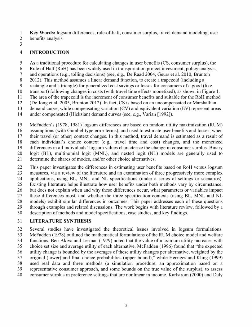
As a traditional procedure for calculating changes in user benefits (CS, consumer surplus), the 5 Rule of Half (RoH) has been widely used in transportation project investment, policy analysis, 6 and operations (e.g., tolling decisions) (see, e.g., De Raad 2004, Geurs et al. 2010, Brunton 7 2012). This method assumes a linear demand function, to create a trapezoid (including a 8 rectangle and a triangle) for generalized cost savings or losses for consumers of a good (like 9 transport) following changes in costs (with travel time effects monetized), as shown in Figure 1. 10 The area of the trapezoid is the increment of consumer benefits and suitable for the RoH method 11 (De Jong et al. 2005, Brunton 2012). In fact, CS is based on an uncompensated or Marshallian 12 demand curve, while compensating variation (CV) and equivalent variation (EV) represent areas 13 under compensated (Hicksian) demand curves (see, e.g., Varian [1992]). 14

McFadden’s (1978, 1981) logsum differences are based on random utility maximization (RUM) 15 assumptions (with Gumbel-type error terms), and used to estimate user benefits and losses, when 16 their travel (or other) context changes. In this method, travel demand is estimated as a result of 17 each individual’s choice context (e.g., travel time and cost) changes, and the monetized 18 differences in all individuals’ logsum values characterize the change in consumer surplus. Binary 19 logit (BL), multinomial logit (MNL), and nested logit (NL) models are generally used to 20 determine the shares of modes, and/or other choice alternatives. 21

This paper investigates the differences in estimating user benefits based on RoH versus logsum 22 measures, via a review of the literature and an examination of three progressively more complex 23 applications, using BL, MNL and NL specifications (under a series of settings or scenarios). 24 Existing literature helps illustrate how user benefits under both methods vary by circumstance, 25 but does not explain when and why these differences occur, what parameters or variables impact 26 these differences most, and whether the three specification contexts (using BL, MNL and NL 27 models) exhibit similar differences in outcomes. This paper addresses each of these questions 28 through examples and related discussions. The work begins with literature review, followed by a 29 description of methods and model specifications, case studies, and key findings. 30

LITERATURE SYNTHESIS 31

Several studies have investigated the theoretical issues involved in logsum formulations. 32 McFadden (1978) outlined the mathematical formulations of the RUM choice model and welfare 33 functions. Ben-Akiva and Lerman (1979) noted that the value of maximum utility increases with 34 choice set size and average utility of each alternative. McFadden (1996) found that “the expected 35 utility change is bounded by the averages of these utility changes per alternative, weighted by the 36 original (lower) and final choice probabilities (upper bound),” while Herriges and Kling (1999) 37 used real data and three methods (a simulation procedure, an approximation based on a 38 representative consumer approach, and some bounds on the true value of the surplus), to assess 39 consumer surplus in preference settings that are nonlinear in income. Karlstrom (2000) and Daly 40

3

(2004) identified conditions for when logsums are appropriate, the foremost of which requires 1 the constant marginal utility of money in the generalized extreme value (GEV) model1. 2

Applications using logsum differences as an evaluation measure have been conducted in Europe, 3 the U.S., and many other countries, for policy and investment decisions in the areas of land use, 4 congestion pricing of roadways, housing location and traffic analysis. For example, the 5 EXPEDITE Consortium (2002) studied the combined effects of an increase in car operating costs 6 and reductions in train and bus/tram/metro costs to illustrate the effects of policy measures. 7 Odeck et al. (2003) used logsums to estimate the relative magnitude of impacts across socio-8 economic groups under Oslo’s cordon toll, based on changes in generalized costs. Castiglione et 9 al. (2003) used San Francisco’s activity-based model and logsum differences to estimate user 10 benefits based on changes in travel costs and induced travel. Gullipali and Kockelman (2008), 11 Gupta et al. (2006), and Kalmanje and Kockelman (2005) used logsum differences to evaluate 12 the impact of credit-based congestion pricing in Texas. 13

The US DOT (2004) compared results of integrated travel demand-land use models to those 14 using demand models only, and used Small and Rosen’ approach (1981) to measure consumer 15 benefit (also known as compensating variation, CV). The authors wondered whether consumer 16 surplus measures for travel demand shifts are still valid when land use demands shift. 17 Essentially, travelers can offset some negative system effects or exploit transport system 18 improvements by moving their home origins, resulting in different (hopefully less negative) 19 welfare implications, but land prices also can change to offset travel benefits, resulting in higher 20 rents. Ma and Kockelman (2014) have a new investigation on such impacts. 21

Finally, Geurs et al.’s (2010) evaluations of Netherland’s data (to anticipate climate change 22 impacts and evaluate potential land-use strategies) suggest that logsum differences help value 23 benefits from changes in trip production and destination utility, which may be quite large and are 24 not measured using the RoH (since RoH assumes that all accessibility benefits accruing to 25 economic agents are attributable to generalized cost changes within the transport system). In this 26 case, logsum and RoH accessibility benefits from the additional road-investment package are 27 quite different (e.g., $148 versus $247 million per year, across 1,000 persons), but on the same 28 order-of-magnitude. In contrast, their differences across the different land-use scenarios were 29 very far apart ($27M versus $697M per year), suggesting that more welfare-characterization 30 research recognizing land use’s welfare impacts may be needed. Most recently, Delle Site and 31 Salucci (2013) proposed welfare calculation methods in the presence of before-after correlations 32 (of the error terms in choice-related utilities), and their example delivered a close correspondence 33 in logsum differences versus RoH values (i.e., 16.41 vs. 16.46 euros per month). 34

Logsum differences come from RUM behaviors, and BL, MNL and NL behavioral specifications 35 are used to anticipate demand changes in most of the literature surveyed here. However, other 36 choice behaviors may dominate. To investigate this idea, Chorus (2010) evaluated route choices 37 under variable travel time, congestion levels, crash exposure, and travel costs, using both RRM 38 (Random Regret Minimization) and RUM (Random Utility Maximization) bases for the MNL 39 specification. He relied on stated preference survey data to compute the logsums which were 40

1 McFadden (1978) noted that, “A random-utility model in which the utilities of the alternatives have independent extreme value distributions yields the Luce (MNL) model. Considering non-independent extreme value distributions leads to the generalized extreme value (GEV) models”.

4

then compared to survey responses (regarding willingness to pay), with only weak correlations 1 found. 2

Kockelman and Lemp (2011) illustrated four-level NL logsum methods (two destinations, three 3 modes, three times of day, and two routes) to equilibrate a toy network’s travel times and choices, 4 and then estimate class-specific user benefits across eight scenarios. They found that road pricing 5 can reduce congestion levels while producing significant and largely positive consumer surplus 6 benefits, though no direct comparisons with RoH valuations were conducted. Brunton (2012) 7 proposed a BL-based example to estimate user benefits in a logsum setting by improving bus 8 transit through decreased travel times, comparing outcomes with RoH estimates, while noting 9 that logsum give a more exact result for consumer surplus than the RoH (which assumes a linear 10 demand relationship). 11

Koopmans and Kroes (2004) and De Raad (2004) compared logsum-based estimates of CS with 12 traditional vehicle-hours-lost (VHL) values, and found logsum method give a higher benefits and 13 increase less rapidly with increasing congestion level than the traditional VHL method. De Jong2 14 et al.’s (2005) comprehensive survey of logsum and RoH comparison results concluded that 15 traditional RoH evaluations should be replaced by logsum differences, to account for non-linear 16 demand assumptions. Brunton’s (2012) example drew a similar conclusion. However, each of 17 these conclusions were based on singular specific scenario examples (e.g., combined project 18 impacts from bus improvements, enhanced capacity, and road toll policy were not evaluated 19 simultaneously in combination in any of the scenarios). 20

Although several works suggest that logsum differences are better than the RoH when valuing 21 user benefits (De Jong et al. 2005; Kockelman and Lemp 2011; Brunton 2012), they also 22 recommend further testing, for more confidence in the details of such results. The literature 23 appears somewhat mixed regarding when the RoH method should closely track logsum 24 differences, and when it should give substantially different results. The following sections 25 describe such comparisons. 26

METHODOLOGY: Using Rule of Half to Estimate User Benefits 27

RoH is one traditional measurement for calculating consumer surplus in transport economics. 28 This method assumes that the consumer demand (in this case, transport demand) curve is linear 29 with respect to generalized costs, at least within the changing context between original and new 30 scenarios. As shown in Figure 1, when generalized cost changes from GC0 to GC1, travel 31 demand in the form of person-trips is assumed to respond accordingly by changing from T0 to T1. 32 Therefore, the change in consumer surplus (∆CS) is denoted by the shaded area of the trapezoid. 33

In accordance with Figure 1’s illustration, ∆CS can be computed as follows: 34

∆ (1) 35

where CS denotes consumer surplus, T0 andT1 are, respectively, the transportation demand before 36 and after a change in scenario context (e.g., tolling changes and/or capacity additions), and GC0 37 and GC1 are the generalized costs before and after the change, respectively. 38 2 This is a survey article, describing much of the research and many applications using logsum methods before the year 2004.

5

Using logsum to estimate user benefits (consumer surplus) 1

The purpose of measuring consumer surplus change is usually to evaluate the social welfare 2 implications resulting from a particular policy or project (De Jong et al. 2005). Since consumer 3 surplus is usually associated with a set of alternatives, when using a logit model with RUM 4 assumption, the change in consumer surplus is calculated as the difference between the expected 5 consumer surplus E(CSn) before and after the change in context (or across scenarios). This 6 procedure relies on the indirect utility of choice alternatives, and is formulated as follows: 7

, ∀n, i (2) 8

where superscript 0 and 1 refer to before and after the change, αn represents the marginal utility 9 of income for person n, and can also be expressed dUn/dYn (assumed to be constant in subsequent 10 case studies investigated here), where Yn is the income of person n, Unis the overall utility for 11 person n, Vn is the indirect utility for person n, and i denotes the choice alternatives available to 12 person n . Therefore, Uni is the overall utility for person n choosing alternative i, and Vni denotes 13 the systematic or representative utility for person n choosing alternative i.

14

This procedure also determines the probabilities that a given person will choose each of the 15 alternatives by using a logit model. These probabilities are estimated by evaluating alternative 16 characteristics in order to assess an indirect utility associated with that alternative. In a MNL 17 model, it is expressed using the following formula: 18

(3) 19

where Pi is the probability of a traveler choosing alternative i from alternative choice set K; and 20 Vi is the indirect utility of alternative i, which is usually a linear function of the attributions of 21 mode i that describe its attractiveness. When using a BL model, the only difference is that the 22 choice set contains just two alternatives. NL models are more complicated than BL and MNL 23 model specifications due to the nested structure and typically greater number of alternatives. 24 However, Equation 3 is the basis of NL within-nest choice decisions, and therefore this equation 25 still governs much of the NL’s behavior. 26

CASE STUDIES 27

In order to fully appreciate the differences between consumer surplus impacts when using 28 logsum and RoH methodologies to estimate user benefits, three broad model categories (BL, 29 MNL and NL models) were investigated here, with several settings or scenarios explored for 30 each model. 31

RoH and Logsum Valuation Comparisons using a Binary Logit Model 32

Brunton (2012) developed a case study assuming 1,000 people traveling from point A to point B. 33 The journey was assumed to take 18 minutes by bus and 10 minutes by car, with assumed 34 VOTTs at $12/hour. Under this scenario, user benefits were calculated from potential decreases 35 in bus travel time using both RoH and logsum methodologies, assuming a BL model. In order to 36 comprehensively assess the difference when using logsum and RoH methodologies, 37

)]ln())[ln(/1()(01

i

V

i

Vnn

nini eeCSE

K

i

VVi

ii eeP1

/

6

improvements in bus travel times (from 1 to 17 minutes) were investigated here, with outcomes 1 shown in Table 1. 2

The BL model’s basic specification and user benefits changes (using logsum methodologies) are 3 expressed as follows: 4

(4) 5

(5) 6

where Pi, Vi,ΔE(CSn) are the same meanings as above, superscript 0 and 1 refer to before and 7 after the bus travel time improvements, GC is generalized cost (in cents), and λ is scaled 8 parameter (assumed here to be -0.03, as in Brunton’s example). 9

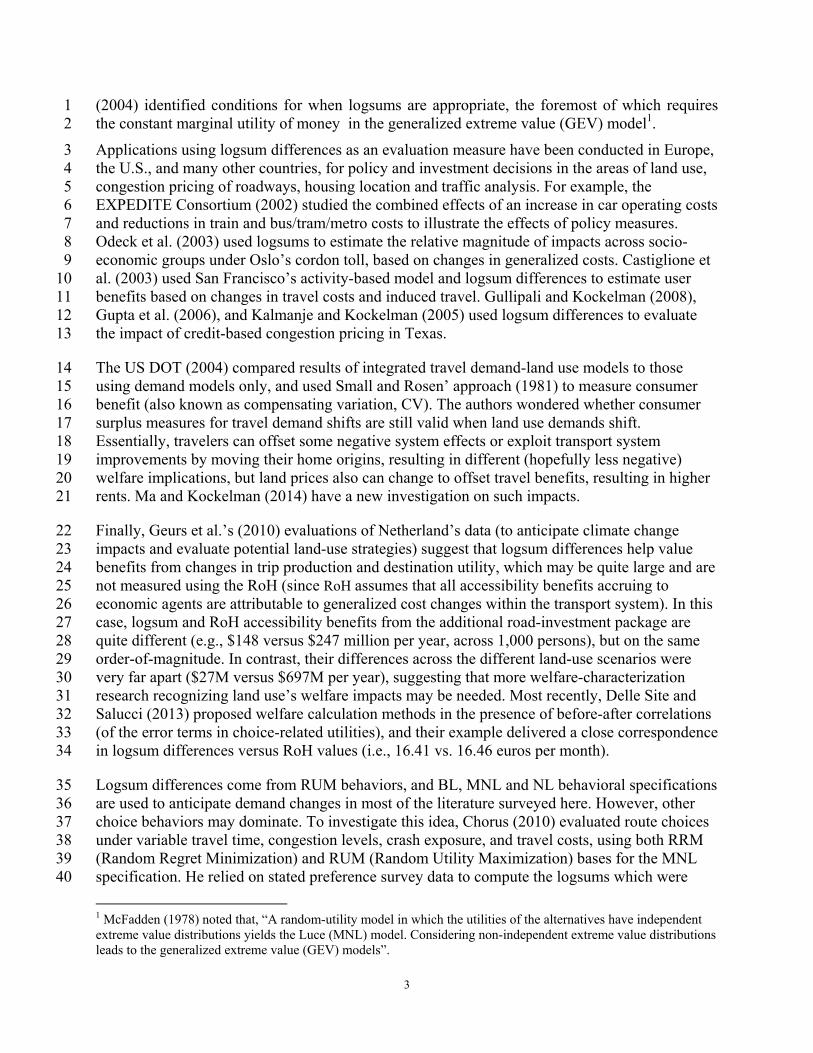
Figure 2 (-a1, -b1, and –c1) illustrates the differences between RoH and logsum calculations, 10 along with estimated bus travel shares as bus travel times fall (-a2, -b2, and –c2), all else equal. 11

Figure 2-a2, shows how the share of bus users increases non-linearly as bus travel times fall, 12 with its graph effectively representing a demand curve (and rotated 90 degrees). The point at 13 which logsum and RoH valuations become equal as bus travel times fall is highlighted by the 14 green dotted line that crosses the curve. This point is critical when comparing RoH- or logsum-15 based benefits (Figure 2-a1). Before this point, the differences between RoH and logsum 16 methodologies present a trend of small-large-small (with a maximum difference of $178.20 per 17 day, or 43.8% in the two valuations [for the 1,000 travelers]) - when bus and car travel times are 18 equal), until reaching Figure 2-a’s green dotted line (the point at which bus travel time is 8 19 minutes less than car travel time, the reverse of the initial scenario). In addition, the logsum 20 benefits curve is lower than the RoH benefits curve, meaning the benefits calculated using 21 logsum differences are lower than those calculated using the RoH. After the inflection point the 22 opposite is true, and differences between the two methodologies become larger again, with the 23 logsum benefits curve higher than the RoH benefits curve. Readers should note that under these 24 circumstances bus travel time is less than 20% of car travel time, an unlikely scenario. However, 25 the binary logit model is structured such that the same results would be obtained for identical bus 26 travel time reductions explored here, even if the initial travel times were 28 and 20 minutes, 27 respectively, for bus and car travel, given that the scale parameter was unchanged. 28

Various λ are investigated here, to determine parameters’ effects on the RoH and logsum values, 29 and their differences (Figure 2). When λ = -0.01 (Figure 2b), the share of bus users almost linear 30 with respect to change in the travel time, and user benefits calculated by RoH and logsum 31 differences are almost identical (with maximum variations between the two of just 4.9% or $32 32 per day, total across 1000 travelers). When λ = -0.05 (Figure 2c), the situation is similar to λ=-33 0.03, except that the differences between RoH and logsum valuations is even larger (with 34 maximum variations growing to 66.8% or $126, over the 1000 affected travelers). Scale 35 parameters (λs) with values of -0.001, -0.005, -0.1 are also investigated here, as shown in Table 36 1. 37

From these results, we can draw the following conclusions: 38

1. If bus percentage grows approximately linearly with decreasing travel times, the benefits 39 calculated by RoH and logsum differences will be very close. 40

i

ii VV )exp()exp( i

ii GCGC )exp()exp(

)]ln())[ln(/1()(01

i

iGC

i

iGCn eeCSE

7

2. Under most circumstances, RoH-calculated benefits are larger than those calculated using 1 logsums, though in extreme cases (like in the very low bus travel times BL scenario), RoH 2 methods may result in smaller user benefits than logsum differences. This should generally 3 hold true when persons shift from one high-use alternative to a lower-use alternative, as the 4 costs of the second alternative fall. 5

3. Figures 2a, 2b, and 2c show the same trend of the differences between RoH and logsum 6 valuations, and the differences grow as λ increases in magnitude. When λ lies near zero (e.g., 7 λ = -0.001 to -0.002), the ratios of logsum/RoH approach 1.0, meaning that the benefits 8 calculated by RoH and logsums are almost the same. When λ grows in magnitude (e.g., λ = -9 0.1), the differences between RoH and logsums become much more substantial. 10

RoH and Logsum Valuation Comparisons using a Multinomial Logit Model 11

Equation 3 noted previously shows the formula used to estimate the probability that a traveler 12 would select a given mode when applying a MNL model. Among this equation, indirect utility, 13 Vi, is generally estimated as a linear function. Here, Equation 6 shows one common expression 14 for indirect utility (from NCHRP Report 365 [Martin and McGuckin, 1998]):. 15

(6) 16

where IVTTi represents the in-vehicle travel time of mode i (in minutes), OVTTi represents the 17 out-of-vehicle travel time of mode i (include walk, wait and transfer times, in minutes), COSTi 18 denotes the out-of-pocket cost of mode i (in dollars), ai, bi, ci, and di are all constant coefficients. 19

Assume that there are 3 modes (Car, Bus, Metro) travelers can choose when they travel from 20 origin O to destination D, where the distance between O and D is 15 miles. Bus and Metro 21 speeds are assumed to be the same as the Car speed (50 mph), however, flat 20 minute and 15 22 minute penalties are added to Bus and Metro times respectively, to represent their added wait, 23 access, and egress times. Further, bus fare is set at $0.50 per trip, metro fare is set at $2 per trip, 24 and a fixed $0.20/mile Car operating cost is assumed3, with a $1.0 parking fee per trip. Therefore, 25 the total Bus travel time is 38 minutes (IVTT 18 min and OVTT 20 min), with $0.50 out of 26 pocket costs; the total Metro travel time is 33 minutes (IVTT 18 min and OVTT 15 min), with 27 $2.00 out of pocket costs; and total Car travel time is 18 minutes (only the IVTT), with $4.00 out 28 of pocket costs. Alternative specific constants (ai) are assumed to be 0.0 for Car, -1.8 for Bus, 29 and -2.0 for Metro, with bi = -0.025, ci = -0.050, and di = -0.004 (Martin and McGuckin, 1998). 30 An average income of $35,000/year, 2080 working-hours/year, and a value of time equal to 25% 31 of income were also assumed, resulting in a VOTT = $16.80/hour. 32

10,000 travelers are assumed here, with no appreciable congestion or bus capacity limitations. 33 That is, the available roadway capacity is large enough such that travel speeds are not impacted, 34 and travelers who shift to the Bus or Metro modes can always find a space. In this scenario, the 35 probabilities of a traveler selecting each mode are calculated, with the Car mode share (0.72) 36 being the largest, due to its relatively high utility. Additionally, four other scenarios are 37 investigated to illustrate the differences in estimated user benefits compared to the base case 38 scenario: Scenario 1 decreases Bus wait times, from the current 18 minutes to just 2-minute waits; 39 Scenario 2 simultaneously decreases Bus and Metro wait times, by 2 minutes each across 6 40 3 Kockelman and Lemp (2011, p. 828) assumed $0.20/mile operating costs, noting that it is “less than the American Automobile Association (AAA 2006) recognizes for full-cost accounting of vehicle ownership and use but about 35% more than current gas costs, assuming a 20 mi/gallon vehicle”.

iiiiiiii COSTdOVVTcIVVTbaV

8

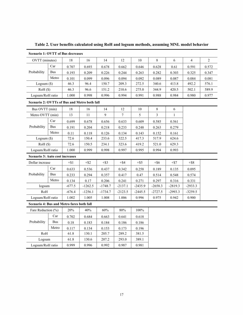
progressive reductions; Scenario 3 increases Car operating costs from $1 to $8, and Scenario 4 1 simultaneously decreases Bus and Metro out-of-pocket costs from the present fares to free rides. 2 As previously noted, logsum-estimated user benefits are calculated using Equation 5.Table 2 3 shows how decreasing Bus OVTTs reduce overall travel times and increase bus shares. There are 4 slight differences between the benefits evaluated using logsum and RoH methodologies, and the 5 RoH is a little larger than the Logsums (Scenario 1). The other three scenarios present similar 6 situations, with just slight differences between logsum and RoH methodology outcomes. This 7 being noted, the magnitude of these differences grows larger with greater changes from the base-8 case scenario. 9

bi, ci and di parameter values were also changed from -0.025, -0.050 and -0.004, to -0.05, -0.1 10 and -0.008, respectively. The results show similar trends (larger parameter values result in 11 greater differences between logsum and RoH valuations), which is largely due the impacts of 12 travel cost growing. 13

RoH and Logsum Valuation Comparisons Using a Nested Logit Model 14

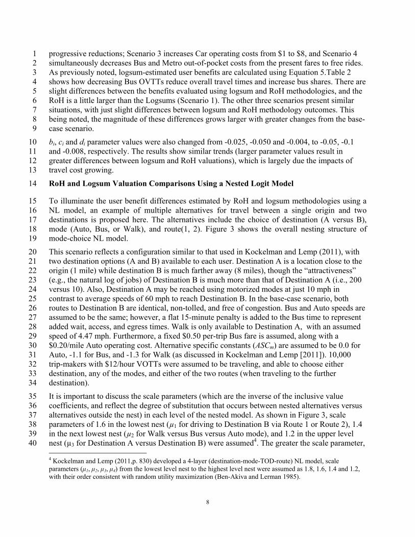
To illuminate the user benefit differences estimated by RoH and logsum methodologies using a 15 NL model, an example of multiple alternatives for travel between a single origin and two 16 destinations is proposed here. The alternatives include the choice of destination (A versus B), 17 mode (Auto, Bus, or Walk), and route(1, 2). Figure 3 shows the overall nesting structure of 18 mode-choice NL model. 19

This scenario reflects a configuration similar to that used in Kockelman and Lemp (2011), with 20 two destination options (A and B) available to each user. Destination A is a location close to the 21 origin (1 mile) while destination B is much farther away (8 miles), though the “attractiveness” 22 (e.g., the natural log of jobs) of Destination B is much more than that of Destination A (i.e., 200 23 versus 10). Also, Destination A may be reached using motorized modes at just 10 mph in 24 contrast to average speeds of 60 mph to reach Destination B. In the base-case scenario, both 25 routes to Destination B are identical, non-tolled, and free of congestion. Bus and Auto speeds are 26 assumed to be the same; however, a flat 15-minute penalty is added to the Bus time to represent 27 added wait, access, and egress times. Walk is only available to Destination A, with an assumed 28 speed of 4.47 mph. Furthermore, a fixed $0.50 per-trip Bus fare is assumed, along with a 29 $0.20/mile Auto operating cost. Alternative specific constants (ASCm) are assumed to be 0.0 for 30 Auto, -1.1 for Bus, and -1.3 for Walk (as discussed in Kockelman and Lemp [2011]). 10,000 31 trip-makers with $12/hour VOTTs were assumed to be traveling, and able to choose either 32 destination, any of the modes, and either of the two routes (when traveling to the further 33 destination). 34

It is important to discuss the scale parameters (which are the inverse of the inclusive value 35 coefficients, and reflect the degree of substitution that occurs between nested alternatives versus 36 alternatives outside the nest) in each level of the nested model. As shown in Figure 3, scale 37 parameters of 1.6 in the lowest nest (µ1 for driving to Destination B via Route 1 or Route 2), 1.4 38 in the next lowest nest (µ2 for Walk versus Bus versus Auto mode), and 1.2 in the upper level 39 nest (µ3 for Destination A versus Destination B) were assumed4. The greater the scale parameter, 40 4 Kockelman and Lemp (2011,p. 830) developed a 4-layer (destination-mode-TOD-route) NL model, scale parameters (μ1, μ2, μ3, μ4) from the lowest level nest to the highest level nest were assumed as 1.8, 1.6, 1.4 and 1.2, with their order consistent with random utility maximization (Ben-Akiva and Lerman 1985).

9

the greater the substitutability among nested alternatives, versus other alternatives. Then, the 1 associated equations, for generalized trip costs, systematic utilities, inclusive values of the nested 2 choices and choice probabilities are as follows: 3

(7) 4

(8) 5

(9) 6

(10)7

(11) 8

(12) 9

(13) 10

Here, GC is the generalized cost, V stands for systematic utility of the alternative (as measured in 11 dollars), denotes the inclusive value or expected maximum utility for an upper level 12 alternative, Pr(·) represents the probability of a particular choice, d, m and r denote Destination 13 (A, B), Mode (Auto, Bus, Walk) and Route (Route1, Route2). VOTT denotes the value of travel 14 time, μ1, μ2, and μ3 are scale parameters for the Route, Mode, and Destination, respectively, 15 COST represents the out-of-pocket travel costs (include fare, toll and operating cost) and has no 16 coefficient (so that utilities are in dollars), IVTT and OVTT denote the travel time spent in and 17 out of the vehicle, attr characterizes the “attractiveness” of each destinations (and attrB is the 18 “attractiveness” of destination B), and ASCm represents the mode-specific (alternative-specific) 19 constants. 20

Consumer surplus change estimates (ΔCS) for each scenario were also computed. The ΔCS 21 computation using normalized logsums of systematic utilities are estimated as follows: 22

(14) 23

While ΔCS can be measured between any two scenarios, this investigation examines changes in 24 consumer surplus relative to the base-case scenario. 25

The base-case scenario assumes two identical, congestion-free, non-tolled routes to Destination 26 B, with scenario summary results (including destination, mode and route choice probabilities) 27 shown in Table 3. Then, In order to compare the differences between user benefits using RoH 28 and logsum methodologies when relying on a NL model, six distinctive alternative scenarios are 29 investigated. Scenario 1 assesses flat tolls on one of the routes to Destination B at rates varying 30

dmrdmrdmrdmr IVTTG COSTVOTTOVTTVOTTC

dmrmdmr GC-A)ln(-)ln(V SCattrattr Bd

)]exp()ln[exp(1

2routedm11routedm11

dm ，， VV

)]exp()exp()ln[exp(1

Walk,d3Bus,d2Autod,22

d VVV

D3

d3d )exp(

)exp(Pr

jj

Mjdj2

dm2ddm )exp(

)exp(PrPr

Rjdmj1

dmr1dmdmr )Vexp(

)Vexp(PrPr

]})exp(ln[-)exp({ln[1

CDd

d0

3Dd

13

3

dS

10

between $0.10 and $0.50 per mile. Scenario 2 explores the impacts of VOTT based on a fix toll-1 rate ($0.20 per mile). Scenario 3 evaluates the impacts of varying operating speeds (from 20 mph 2 to 80 mph, Route 2 to Destination B), reflecting potential roadway facility upgrades with higher 3 speeds or worsening overall congestion with lower speeds. Scenario 4 changes bus wait times 4 reflecting policies that increase or decrease the level-of-service for public transit, while Scenario 5 5 alters bus fares. Scenario 6 varies auto operating costs, reflecting changing gasoline prices and 6 parking fees. 7

Each scenario assumes 10,000 persons who want to travel (to Destination A or B), and with user 8 benefits compared across scenarios (relative to base-case scenario), using RoH and logsum 9 methodologies, with results shown in Table 4. 10

Results show that the benefits calculated when using logsum versus RoH methodologies differ 11 more substantially with travel time changes, and the differences become more significant in 12 Scenario 1 when a route is tolled. When Autos are tolled on Route 2 to Destination B in Scenario 13 1, the difference between the two become larger with increased toll-rates, with logsums 14 valuations typically smaller than RoH valuations. In Scenario 2, when changing the VOTT from 15 $1/hr to $12/hr, the logsum/RoH ratio rises from 0.761 to 0.822, suggesting that higher values of 16 time may lead to more consistent results in logsum and RoH valuations. In Scenario 3,when 17 altering the speed from 20 mph to 80 mph on Route 2 to Destination B, the logsum/ RoH ratios 18 rise, and they are greater than/less than 1.0 when the base-case speed is greater than/less than 60 19 mph. The user benefits evaluated using logsum and RoH methodologies are closer when travel 20 speeds change modestly, from 50 mph and 70 mph, rather than more dramatically. In Scenario 4, 21 the logsum/RoH ratios fall as the Bus OVTT change increases. In Scenarios 5 and 6 (which vary 22 Bus fares and Auto operating costs), there are only slight differences between the two methods 23 for calculating user benefits. 24

Analysis of the 3 Cases 25

In analyzing the results of these 3 cases and their associated scenarios, the following conclusions 26 can be drawn: 27

1. As the magnitude of parameters and variables in utility expression grow, the percentile and 28 absolute differences between logsum and RoH valuations become larger. 29

2. With slight changes in travel time, travel cost and other variables, the percentile and absolute 30 differences between logsum and RoH valuations are very small; but these differences grow 31 as the alternative scenario increasingly diverges from the base-case scenario. Also, when 32 travel demand is a near-linear function of travel time and other variables, the user benefits 33 calculated using RoH and logsum methodologies are close. 34

3. Under most circumstances, the magnitude of the impacts (including negative user benefit 35 valuations) calculated using RoH are larger than using logsum differences. However, in some 36 instances RoH may be smaller than Logsum differences (e.g., when the changes in travel cost 37 are very large, compared to base scenarios). 38

These differences between estimated logsum and RoH valuations may be further illustrated by 39 simultaneously comparing all scenarios and modeling results, providing a useful and quick-40 reference framework for transport planners, managers and decision-makers. Table 5 shows how 41 travel time, travel cost, tolls and other parameters influence the differences between RoH and 42 logsum valuations, as input variables change in sign and magnitude. These input changes reflect 43

11

potential transport policies, projects, and/or management decisions, and may serve as a reference 1 for future planning and decision-making efforts. 2

CONCLUSIONS 3

Much work currently exists on examining logsum differences to estimate potential user benefits 4 from various policies or projects, but existing comparisons between RoH and logsum benefits is 5 largely lacking, particularly in the context of a comprehensive comparison evaluating the 6 impacts of changing travel times, travel costs, added tolls and other important parameters aspects. 7 This paper uses case studies to analyze and summarize the differences between RoH and logsum 8 valuations as a measure of user benefits. As shown using model types, the ratio between logsum 9 and RoH valuations varies on scenario context and the degree to which input parameters change. 10 The tollway scenario illustrates this phenomenon, as the difference in estimated benefits when 11 using these two methodologies becomes larger as toll rates grow. This implies the RoH method 12 may sometimes over-estimate the effects of a given policy, especially when the change is 13 significant compared to the base-case scenario. In these three cases, the differences between RoH 14 and logsum valuations when using the MNL model appear to be smaller than when using either 15 BL or NL models. This is mainly due to the changes in probabilities of each alternative are 16 almost linear or near-linear in MNL model compared in BL and NL models. While this last 17 conclusion is indicated by assessing results from these three specific cases, it is possible that it 18 may not hold under all circumstances, so further research may be needed. 19

Results also indicate that when the transport demand is a linear function, the ratio between 20 logsum and RoH valuations is close to 1, though transport demand usually exhibits nonlinear 21 trends. As such, it is recommended that policy-makers estimate user benefits using logsum 22 valuations when travel time or travel cost impacts are anticipated to be large, since logsums are 23 more accurate than traveler welfare valuations estimated using the RoH methodology. 24

Of course, the analysis provided here illustrates only a limited number of idealized scenarios 25 under three governing model formulations. Many other potential explorations and scenario 26 extensions exist, which could further highlight key issues involved in these differences. For 27 example, other evaluations could examine if multiple inputs simultaneously change (for example, 28 travel times under varying congestion levels and toll prices). In addition, when a given route is 29 tolled, the entire transportation network may be impacted, potentially further influencing 30 differences in logsum and RoH valuations. One could also explore other underlying model 31 structures to generate the demand functions, and investigate which method is more robust to 32 other behavioral assumptions. Linear demand functions are likely to favor the RoH, which was at 33 a disadvantage here (thanks to starting off with a random-utility logit-based model for all choice 34 behaviors). 35

In summary, the comparison evaluating the differences between logsum and RoH valuations 36 should help transportation planners and policy-makers understand how the choice of evaluation 37 methodology will influence and potentially bias the expected benefits from a given project or 38 policy. When relatively minimal impacts are expected to the overall underlying generalized cost 39 of a given choice alternative, the two methods are roughly equivalent. However, when changes 40 in such costs are expected to be substantial, there is a strong chance that using the RoH 41 methodology may produce a substantially mis-estimated result, potentially overestimating or 42 underestimating benefits by up to half. 43

ACKNOWLEDGEMENTS 44

12

Dr. Jason Lemp constructed the original the NL mode-choice model structure, which was 1 modified by the authors for specific scenarios, and he provided some of the reference data at the 2 start of this research. We also appreciate the administrative contributions of Ms. Annette Perrone, 3 the comments of several anonymous reviewers, and the financial support of the China 4 Scholarship Council, which funded the lead author’s one-year stay in the U.S. 5

6

REFERENCES 7

Ben-Akiva, M. and Lerman, S. R., 1979. Disaggregate travel and mobility choice models and 8 measures of accessibility, in Hensher, D. A. and Stopher, P. R. (eds.) Behavioural Travel 9 Modelling, Croom Helm. 10

Ben-Akiva, M., Lerman, S. 1985. Discrete Choice Analysis: Theory and Application to Travel 11 Demand. MIT Press. 12

Brunton P., 2012. Transport User Benefits: An Alternative to the Rule of Half. Available at 13 http://www.citilabs.com/sites/default/files/files/3_Aecom_Transport%20User%20Benefits.pdf. 14

Castiglione, J., Freedman, J. and Davidson W., 2003. Application of a tour-based 15 microsimulation model to a major transit investment, San Francisco County Transportation 16 Authority and PBConsult, San Francisco. http://www.joecastiglione.com/page4/page4.html 17

Delle Site, P., Salucci, M., 2013. Transition Choice Probabilities and Welfare Analysis in 18 Random Utility Models with Imperfect Before-After Correlation. Transportation Research Part B 19 58: 215-242. 20

Daly, A., 2004. Properties of random utility models of consumer choice, presented to TraLog 21 Conference, Molde. http://www.its.leeds.ac.uk/people/a.daly 22

De Jong, G., Pieters, M., Daly, A., Graafland, I., Kroes, E., Koopmans, C., 2005. Using the 23 Logsum as an Evaluation Measure. Report WR-275-AVV, prepared for AVV Transport 24 Research Centre, RAND Europe. Available at 25 http://www.rand.org/content/dam/rand/pubs/working_papers/2005/RAND_WR275.pdf. 26

EXPEDITE Consortium, 2002. EXPEDITE Final Publishable Report, Report for European 27 Commission, DGTREN, RAND Europe, Leiden. 28 http://www.rand.org/pubs/working_papers/WR275.html 29

Geurs, K., Zondag, B., de Jong, G., de Bok, M., 2010. Accessibility Appraisal of Land-Use / 30 Transport Policy Strategies: More than just Adding up Travel-Time Savings. Transportation 31 Research Part D: 382-393. 32

Gulipalli P. and Kockelman K.M., 2008. Credit-Based Congestion Pricing: A Dallas-Fort Worth 33 Application. Transport Policy 15 (1): 23-32. 34

Gupta, S., Kalmanje S., and Kockelman, K., 2006. Road Pricing Simulations:Traffic, Land Use 35 and Welfare Impacts for Austin, Texas. Transportation Planning and Technology, 29 (1): 1-23. 36

Harris, A. J. and Tanner, J. C., 1974. Transport demand models based on personal characteristics, 37 TRRL Supplementary Report 65 UC. 38

Herriges, J. A. and Kling, C. L., 1999. Non-linear income effects in random utility models, 39 Review of Economics and Statistics 81 (1): 62-72. 40

13

Karlstrom, A., 2000. Non-linear value functions in random utility econometrics. Presented to the 1 IATBR Conference, Gold Coast, Australia. 2 http://onesearch.lib.polyu.edu.hk:1701/primo_library/libweb/action/dlDisplay.do?vid=HKPU&d3 ocId=HKPU_MILLENNIUM16213452&fromSitemap=1&afterPDS=true 4

Koopmans, C.C. and Kroes, E.P., 2004. Werkelijke kosten van files tweemaal zo hoog (The real 5 cost of queues twice as high), Economisch Statistische Berichten 89:154-155. 6

Kalmanje S., Sukumar, and Kockelman K.M., 2004. Credit-based congestion pricing travel, land 7 value, and welfare impacts. Transportation Research Record No. 1864: 45-53. 8

Kockelman K.M., and Kalmanje S., 2005. Credit-based congestion pricing: a policy proposal and 9 the public’s response. Transportation Research Part A: 39 (7-9): 671-690 10

Kockelman K.M., Lemp J.D., 2011.Anticipating new-highway impacts: opportunities for welfare 11 analysis and credit-based congestion pricing. Transportation Research Part A, 45 (8): 825-838. 12

Ma, S., Kockelman, K. 2014. Welfare Measures to Reflect Home Location Options When 13 Transportation Systems are Modified. Paper under review for presentation at the 94th Annual 14 Meeting of the TRB, and for publication in Transportation Research Record. 15

Martin, W., McGuckin, N. 1998. Travel Estimation Techniques for Urban Planning. National 16 Cooperative Highway Research Program (NCHRP) Report 365. National Academy of Science, 17 Washington, D.C. http://onlinepubs.trb.org/onlinepubs/nchrp/nchrp_rpt_365.pdf. 18

McFadden, D., 1978. Modelling the choice of residential location. In Karlqvist, A., Lundqvist, L., 19 Snickars, F. and Weibull, J. (eds) Spatial Interaction Theory and Residential Location. North-20 Holland, Amsterdam. 21

McFadden, D., 1996. On computation of willingness-to-pay in travel demand models, Dept. of 22 Economics, University of California, Berkeley. 23

McFadden, D., 1981. Econometric models of probabilistic choice. In Manski, C. and McFadden, 24 D. (eds) Structural Analysis of Discrete Data: With Econometric Applications. The MIT Press, 25 Cambridge, Massachusetts. 26

Nellthorp J. and Hyman G., Alternatives to the Rule of a Half in Matrix-Based 27 Appraisal,http://www.its.leeds.ac.uk/projects/WBToolkit/Note6Annex1.htm 28

Odeck, J., Rekdal, J. and Hamre, T.N., 2003. The Socio-economic benefits of moving from 29 cordon toll to congestion pricing: The case of Oslo. Paper presented at TRB Annual Meeting, 30 Washington D.C. 31

Raad, P.M. de, 2004. Congestion costs closer examined, Monetarising adaptive behaviour using 32 the Logsum-method. MSc Thesis, TU Delft, The Netherlands. 33

Small, K. A. and Rosen, H. S., 1981. Applied welfare economics with discrete choice models, 34 Econometrica 49:105-130. 35

US Department of Transportation, Federal Highway Administration (2004) Case Study: 36 Sacramento, California Methodology Calculation of User Benefits, USDoT, 37 http://www.fhwa.dot.gov/planning/toolbox/sacramento_methodology_user.htm 38

Varian, H. 1992. Microeconomic Analysis, 3rd Edition. W.W. Norton & Co. 39

14

1

2

3

Figure1. Using rule-of-half (RoH) to estimate user benefits 4

Demand D(GC)

Supply1

Supply0

Trips T

Generalized cost GC

GC0

GC1

T0 T1

15

Table 1 User benefits calculated using RoH and logsum methods, with bus travel time falling (BL model specification)

λ = -0.03

Modes Base scenario Bus travel time decreases (min)

car bus 1 2 3 4 5 6 7 8 9 10 11 12 13 14 15 16 17

Travel time (min)

10 18 17 16 15 14 13 12 11 10 9 8 7 6 5 4 3 2 1

Cost (cents) 200 360 340 320 300 280 260 240 220 200 180 160 140 120 100 80 60 40 20

Probability 0.992 0.008 0.008 0.015 0.027 0.047 0.083 0.141 0.231 0.354 0.500 0.646 0.769 0.858 0.917 0.953 0.973 0.985 0.992

Benefits ($)

RoH 2.3 7.0 16.7 36.5 75.0 143.8 253.8 406.5 588.4 776.7 952.9 1110.0 1249.0 1374.2 1490.1 1600.0 1706.2

Logsum 2.2 6.3 13.5 26.2 48.3 85.0 143.1 228.3 343.1 485.0 648.3 826.2 1013.5 1206.3 1402.2 1600.0 1798.8

Logsum/RoH ratio 0.972 0.900 0.807 0.718 0.643 0.591 0.564 0.562 0.583 0.624 0.680 0.744 0.811 0.878 0.941 1.000 1.054

λ = -0.01

RoH 36.6 79.9 131.1 191.2 261.2 341.6 432.7 534.4 646.0 766.7 895.0 1029.5 1168.8 1311.1 1455.2 1600.0 1744.4

Logsum 36.5 79.4 129.4 187.2 253.6 329.1 414.2 509.2 614.2 729.1 853.6 987.2 1129.4 1279.4 1436.5 1600.0 1769.1

Logsum/RoH ratio 0.998 0.994 0.987 0.979 0.971 0.964 0.957 0.953 0.951 0.951 0.954 0.959 0.966 0.976 0.987 1.000 1.014

λ = -0.05

RoH 0.1 0.6 2.1 7.3 23.9 71.7 188.5 400.3 658.3 881.1 1048.2 1178.8 1291.7 1397.0 1499.1 1600.0 1700.4

Logsum 0.1 0.4 1.3 3.6 9.7 25.3 62.6 138.6 262.6 425.3 609.7 803.6 1001.3 1200.4 1400.1 1600.0 1800.0

Logsum/RoH ratio 0.924 0.762 0.605 0.486 0.404 0.353 0.332 0.346 0.399 0.483 0.582 0.682 0.775 0.859 0.934 1.000 1.059

λ = -0.001, -0.002, -0.005, -0.1

logsum/RoH ratio

λ = -0.001 1.000 1.000 1.000 1.000 1.000 1.000 1.000 1.000 1.000 1.000 1.000 1.000 1.000 1.000 1.000 1.000 1.000

λ = -0.002 1.000 1.000 1.000 1.000 1.000 1.000 1.000 1.000 1.000 1.000 1.000 1.000 1.000 1.000 1.000 1.000 1.000

λ = -0.005 1.000 0.999 0.998 0.998 0.997 0.996 0.995 0.994 0.993 0.993 0.993 0.994 0.995 0.996 0.998 1.000 1.003

λ = -0.1 0.762 0.482 0.332 0.250 0.200 0.168 0.152 0.173 0.268 0.409 0.547 0.667 0.769 0.857 0.933 1.000 1.059

Note: These benefits are calculated for 1,000 people traveling from point A to point B for one trip. Benefits in Figures 2a, 2b, and 2c share this same basis.

16

a1 a2

(a) λ = -0.03

b1 b2

(b) λ = -0.01

c1 c2

(c) λ = -0.05

Figure 2. Total user benefits (per day, across 1000 travelers) calculated using RoH and logsum methods and bus share changes following reductions in bus travel times

17

Table 2. User benefits calculated using RoH and logsum methods, assuming MNL model behavior

Scenario 1: OVTT of Bus decreases

OVTT (minutes) 18 16 14 12 10 8 6 4 2

Probability

Car 0.707 0.693 0.678 0.662 0.646 0.628 0.61 0.591 0.572

Bus 0.193 0.209 0.226 0.244 0.263 0.282 0.303 0.325 0.347

Metro 0.101 0.099 0.096 0.094 0.092 0.089 0.087 0.084 0.081

Logsum ($) 46.3 96.4 150.7 209.3 272.5 340.6 413.8 492.2 576.1

RoH ($) 46.3 96.6 151.2 210.6 275.0 344.9 420.5 502.1 589.9

Logsum/RoH ratio 1.000 0.998 0.996 0.994 0.991 0.988 0.984 0.980 0.977

Scenario 2: OVTTs of Bus and Metro both fall

Bus OVTT (min) 18 16 14 12 10 8 6

Metro OVTT (min) 13 11 9 7 5 3 1

Probability

Car 0.699 0.678 0.656 0.633 0.609 0.585 0.561

Bus 0.191 0.204 0.218 0.233 0.248 0.263 0.279

Metro 0.11 0.118 0.126 0.134 0.143 0.152 0.161

Logsum ($) 72.6 150.4 233.6 322.5 417.3 517.9 624.6

RoH ($) 72.6 150.5 234.1 323.6 419.2 521.0 629.3

Logsum/RoH ratio 1.000 0.999 0.998 0.997 0.995 0.994 0.993

Scenario 3: Auto cost increases

Dollar increase +$1 +$2 +$3 +$4 +$5 +$6 +$7 +$8

Probability

Car 0.633 0.536 0.437 0.342 0.258 0.189 0.135 0.095

Bus 0.233 0.294 0.357 0.417 0.47 0.514 0.548 0.574

Metro 0.134 0.17 0.206 0.241 0.271 0.297 0.316 0.331

logsum -677.5 -1262.5 -1748.7 -2137.1 -2435.9 -2658.3 -2819.3 -2933.3

RoH -676.4 -1256.1 -1734.7 -2123.5 -2445.5 -2727.5 -2993.3 -3259.5

Logsum/RoH ratio 1.002 1.005 1.008 1.006 0.996 0.975 0.942 0.900

Scenario 4: Bus and Metro fares both fall

Fare Reduction (%) 20% 40% 60% 80% 100%

Probability

Car 0.702 0.684 0.663 0.641 0.618

Bus 0.18 0.183 0.184 0.186 0.186

Metro 0.117 0.134 0.153 0.173 0.196

RoH 61.8 130.1 205.7 289.2 381.5

Logsum 61.8 130.6 207.2 293.0 389.1

Logsum/RoH ratio 0.999 0.996 0.992 0.987 0.981

18

Figure 3. Mode-choice NL model structure

Trip

Destination A Destination B

Auto Auto Bus Bus Walk

Route 1 Route 2 Route 1 Route 2

µ1=1.6

µ2=1.4 µ2=1.4

µ3=1.2

19

Table 3. Original settings and calculated probabilities for the base-case scenario (NL model)

Destination Mode Route

Travel time (minutes)

Travel cost （$）

Choice probability

IVTT OVTT Fare Opera.

cost Toll

A

Bus 6 15 0.5 0 0

0.125

0.0003 0.0003

Auto 6 0 0 0.2 0 0.122 0.122

Walk 0 13.4 0 0 0 0.0033 0.0033

B

BusRoute 1 8 15 0.5 0 0

0.875

0.0148 0.0074

Route 2 8 15 0.5 0 0 0.0074

AutoRoute 1 8 0 0 1.6 0

0.860 0.430

Route 2 8 0 0 1.6 0 0.430

dPr dmPr dmrPr

20

Table 4. User benefits calculated using RoH and logsum methodologies using an NL model ($)

Scenario 1

Route 2 to Destination B, where Auto is tolled

Toll (cent/mile) 10 ct/mi. 20 30 40 50 10 20 30 40 50

VOTT $12/hour $6/hour

Logsum -2344.5 -3202.2 -3464.7 -3539.8 -3560.8 -2123.5 -2881 -3110.4 -3175.8 -3194.1

RoH -2427.9 -3895.2 -5358.6 -6954.8 -8626.3 -2212.6 -3564.3 -4921.3 -6395.9 -7936.4

Logsum/RoH ratio 0.965 0.822 0.646 0.509 0.413 0.959 0.808 0.632 0.496 0.402

Scenario 2

Route 2 to Destination B, where Auto is tolled at a fixed rate (20¢/mile ) while considering various VOTTs

VOTT($/hr) 1 2 3 4 5 7 8 9 10 11

Logsum -1741.6 -2030.4 -2298.6 -2533.3 -2727.8 -2996.4 -3079.3 -3136.1 -3172.4 -3193.1

RoH -2288.8 -2626.9 -2931.6 -3191.2 -3401.5 -3685 -3770.8 -3828.9 -3865.7 -3886.5

Logsum/RoH ratio 0.761 0.773 0.784 0.794 0.802 0.813 0.817 0.819 0.821 0.822

Scenario 3

Route 2 to Destination B, with speed variations (Base scenario is 60 mph)

Route2 Speed 20 30 40 50 70 80 90

Logsum -3619.9 -3272.8 -2392.7 -1209.2 1100.6 2057.9 is not

realistic

RoH -7075.6 -3967.1 -2474.8 -1212.7 1100.9 2056.4

Logsum/RoH ratio 0.512 0.824 0.966 0.997 1.00 1.001

Scenario 4

Changed Bus OVTT times (on wait, access, and egress times)

Added time -60%

(6 min) -40%

(9 min) -20%

(12 min) 0

+20% (18 min)

+40% (21 min)

+60% (24 min)

Logsum 1138.1 456.6 140.8 --- -61.7 -88.5 -100.1

RoH 1544.9 536.5 145.5 --- -63.7 -105.8 -144.4

Logsum/RoH ratio 0.737 0.851 0.968 --- 0.965 0.836 0.693

Scenario 5

Changed Bus fare (decrease and increase)

Decrease/Increase -100% -80% -60% -40% -20% +20% +40% +60% +80% +100%

Logsum 108.7 80.7 56.2 34.8 16.2 -14.1 -26.4 -37.2 -46.5 -54.6

RoH 110.6 81.0 55.8 34.4 15.9 -13.9 -26.1 -36.9 -46.7 -55.6

Logsum/ RoH ratio 0.983 0.996 1.006 1.014 1.018 1.018 1.014 1.006 0.995 0.981

Scenario 6

Change Auto (car) operating costs (decrease and increase)

Decrease/Increase -20% -40% -60% -80% +20% +40% +60% +80% +100%

Logsum 2856.2 5804.9 8822.8 11891.7 -2734.9 -5315.4 -7705.9 -9873.0 -11790

RoH 2847.6 5765.6 8726.5 11711.4 -2732.1 -5292.2 -7627.1 -9692.8 -11468

Logsum/RoH ratio 1.003 1.007 1.011 1.015 1.001 1.004 1.010 1.019 1.028

21

Table 5. Summary of the comparation of RoH and logsum methodologies

Logsum/RoH Parameter Travel Time Travel Cost Toll Curve of

Logsum/RoH with Change Increase

Relevant Policy

BL model

= -0.001 1.0

public transport priority

speed control

toll or road pricing

travel mode cost change

= -0.005 0.993-1.003

= -0.03 0.562-1.054

= -0.05 0.332-1.059

= -0.1 0.173-1.059

MNL model

bi = -0.05, ci = -0.01, di = -0.008

0.980-0.999 0.506-1.003

bi = -0.025, ci = -0.05, di = -0.004

0.977-1.0 0.900-1.008

bi = -0.0125, ci =-0.025, di = -0.002

0.991-1.0 1.0-1.011

NL model

0.402-0.965

0.512-1.001

0.983-1.028

6.11

4.12

2.13