1

Time-Correlation Functions

Charusita ChakravartyIndian Institute of Technology Delhi

2

Organization• Time Correlation Function: Definitions and Properties• Linear Response Theory :

– Fluctuation-Dissipation Theorem– Onsager’s Regression Hypothesis– Response Functions

• Chemical Kinetics• Transport Properties

– Self-diffusivity– Ionic Conductivity– Viscosity

• Absorption of Electromagnetic Radiation• Space-time Correlation Functions

3

Time Correlation Functions

• Time-dependent trajectory of a classical system:• Since the classical system is deterministic, a time-dependentquantity can be written as :

• Correlation function as a time average over a trajectory:

average Time )()(1

)(

tyStationari )"()'(1

)'"(

average Time )"()'(1

)",'(

0

0

0

dtBALttC

dtBtALtttC

dtBtALtttC

))(),(( tptr

);,());0(),0(())(),(()( tprAtprAtptrAtA

4

• Time-correlation functions can be written as ensemble averages by summing over all possible initial conditions:

Probability of observing a microstate

• Limiting behaviour

• Alternative definition of time-correlation function in terms of deviations of time-dependent properties from mean values.

)),(exp(/)),(exp(),( prHpdrdprHprP

)()0();,()0;,(),()( tBAtprBprAprPpdrdtC

BAtCt

ABtCt

tBAtC

)( ,When

)( ,0When

)()0()(

0)( ,When

1)( ,0When

)0()0(/)()0()('

tCt

tCt

AA(t)-δA(t)

BAtBAtC

5

• Stationarity for systems with continuous interparticle forces, TCFs must be even functions of the time delay:

• Time-derivative with respect to time origins must be zero

• Short-time expansion of autocorrelation functions

)()( tCtC

)0()()()()()0( BtAstBsAtBA

)()()()(

0)()(

stBsAstBsA

tsBsAds

d

....)0()0()2/1()( 2 AAAtC

6

Typical velocity autocorrelation function

Zero slope at origin

Rebound fromSolvent cage

D. Chandler

7

Small Deviations from Equilibrium:Classical Linear Response Theory

• Apply a weak perturbing field f to the system that couples to some physical property of the system– Electric field/ionic motion– Electromagnetic radiation/charges or molecular dipoles

System prepared in non-equilibriumstate by applying perturbing field f

System allowed to relax freely

Equilibrium established

),(),( prfAprH

),( prH

),( prHtime=0

B(t)

D. Chandler

8

Linear Response Theory (contd.)• Let the time-dependent perturbation be such that

• At t=0, the probability of observing a configuration:

• How will the observed value of a quantity B(t) change with time when the perturbation is turned off at time t=0?

)),(exp(/)),(exp(),( fAprHpdrdfAprHprF

)0;,(),()( tprBprFpdrdtB

Integrate over initial conditions of perturbed system at t=0

Time-dependent value of B for a given set of initial conditions

0for 0

0for 1)(

t

ttf

9

Linear Response Theory (contd.)Consider the effect of perturbations only upto first-order:

fAH

fAHfAprH

1)exp(

)exp()exp()),(exp(

D. Chandler, Introduction to Modern Statistical Mechanics

10

• For t>0, the observed value of B will be given by

• Multiply the numerator and denominator by (1/Q) where Q is the partition function of the unperturbed system

• Denominator )exp( HpdrdQ

fAHpdrd

tBfAHpdrd

tprBprFpdrdtB

1)exp(

)(1)exp(

);,(),()(

Af

HpdrdAHpdrdfHpdrd

fAHpdrdQ

1

)exp(/)exp()exp(

1)exp()/1(

11

)()0(

)()0()exp()/1()()exp()/1(

)(1)exp()/1(

tBAfB

tBAHpdrdQftBHpdrdQ

tBfAHpdrdQ

Numerator:

BAftBAfB

AftBAfB

fAtBAfBtB

)()0(

....1)()0(

1)()0()( 1

Time-dependent behaviour of B:

12

Onsager’s regression hypothesis

The relaxation of macroscopic non-equilibrium disturbances is governed by the same dynamics as the regression of spontaneous microscopic fluctuations in the equilibrium system

BAtBAfBtB )()0()(

)()0()( tBAftB

Macroscopic relaxation

Equilibrium Time-correlation function

13

Response Functions

For a weak perturbation , we can define a response function:

The response of the system to an impulsive perturbation:

To correspond to the linear response situation studied earlier:

BAtABfAtAtA )()0()()(

)'()',(')( tfttdttA AB

)'()',(')(),( 00 ttttdttAtt ABAB

)'( )',( :tyStationari

'for 0)',( :Causality

tttt

tttt

ABAB

AB

otherwise 0)'( and 0for )'( tftftf

t

ABAB dfttdtftA )()'(')(0

14

• Provides an alternative route to evaluate the time-dependent response as an integral over a time-correlation function

)()0()(

0for 0

0for )()0()(

)()()0()(

ABdftA

t

ttAB

dfBAtABftA

t

AB

t

AB

15

Transport Properties• Flux=-transport coefficient X gradient• Non-equilibrium MD: create a perturbation and watch the

time-dependent response• Equilibrium MD: measure the time-correlation function

Flux Gradient Linear Laws

Diffusivity Mass Concentration Fick’s Law of Diffusion

Ionic Conductivity

Charge Electric potential Ohm’s Law

Viscosity Momentum Velocity Newton’s Law of Viscosity

ThermalConductivity

Energy Temperature Fourier’s Law of Heat Conduction

16

Self-diffusivityConsider an external field that couples to the position of a

tagged particle such that

The steady state velocity of the tagged particle will then be:xxFHH 0'

0

0

0

)()0(

)()0(

)(

)'('

mobility theis where)(

xxx

xx

xvx

xvx

xx

vvdF

vxdF

dF

ttdtF

Ftv

x

x

17

Can one identify the mobility, as defined below, with the macroscopic velocity:

Fick’s Law: Flux of diffusing species= Diffusivity X Concentration gradient

Combining with the equation of continuity derived by imposing conservation of mass of tagged particles, gives :

Diffusion Equation

0

)()0( xxx vvd

),( trcDj

0),(),(

0),(),(

2

trcDt

trc

trjt

trc

18

If the original concentration profile is a delta-function, then the concentration profile at a later time (t) will be a d-dimensional Gaussian:

Consider the second-moment of one-dimensional distribution:

Einstein relation

By writing the displacement as

one can show that

This definition of self-diffusivity will be the same as that of the mobility derived from linear reponse theory

))4/(exp()4/(1),(

)()0,(22/ DtrDttrc

rrcd

Dtxtx 2)0()(2

Dtrtr 6)0()(2

t

iii dttvrtr0

')'()0()(

0

2)()0(6)0()( xx vvdtrtr

19

Ionic ConductivityConsider an external electric field Ex applied to an ionic melt. Under

steady state conditions, the system will develop a net current:

The ionic conductivity per unit volume, will be defined by:

Effect of the external field on the Hamiltonian:

When the field is switched off at t=0, the current will decay towards the zero value characteristic of the unperturbed system.

)()()( tMtreztj xii

ix

Charge on particle i

velocity particle i

Rate of change of netdipole moment

xx VEtj )(

xxEMHH 0'

20

To apply the relation:

to compute the time-dependent decay of the current, we set:

to obtain:

Conductivity per unit volume will then be given by:

)()0()( tABdftAt

xx MBjA and

)()0(

)()0()(

0

0

MMdE

MMdEtj

x

xx

)()0(1)(

0

xxBx

x jjdTVkVE

tj

21

Collective Transport Properties Silica (6000K, 3.0 g/cc)

Ionic Conductivity Viscosity

22

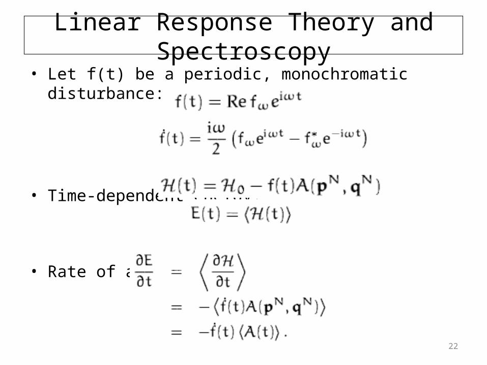
Linear Response Theory and Spectroscopy• Let f(t) be a periodic, monochromatic disturbance:

• Time-dependent energy:

• Rate of absorption of energy:

23

Linear Response Theory and Spectroscopy (contd.)

• Time-dependent value of A reflects response to applied field:

• The average rate of absorption or energy dissipation is given by:

• For a periodic field:

24

Linear Response Theory and Spectroscopy (contd.)• Fourier transform of response function is defined as:

• Compute average rate of absorption of energy over one time period T=

25

Linear Response Theory and Spectroscopy (contd.)

• Using linear response theory

• Absorption spectrum

26

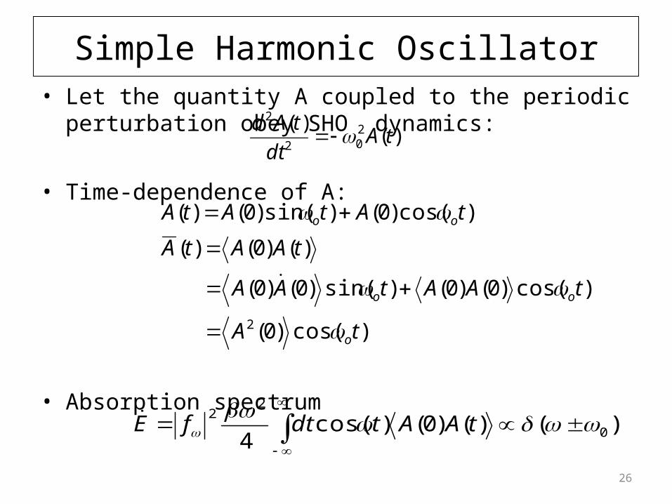
Simple Harmonic Oscillator• Let the quantity A coupled to the periodic perturbation obey

SHO dynamics:

• Time-dependence of A:

• Absorption spectrum

)()( 2

02

2

tAdt

tAd

)cos()0(

)cos()0()0()sin()0()0(

)()0()(

)cos()0()sin()0()(

2 tA

tAAtAA

tAAtA

tAtAtA

o

oo

oo

)()()0()cos(4 0

22

tAAtdtfE

27

Infrared Absorption by a Dilute Gas of Polar Molecules

• X-component of total dipole moment will couple to oscillating electric field .

• Independent dipole approximation:• Perturbed Hamiltonian:

• Change in dipole moment with time:

• Thermal distribution of angular velocities, P(), will be reflected in absorption profile

i

ixM

)()( 0 tEMHtH xx

)cos()3/()()0(3

)()0()()0()()0(

2 tNt)(N/

tttMMi

ixixi j

jxixxx

28

Spectroscopic Techniques

Technique Time-correlation Function

Dynamical quantity

Dielectric relaxation

Unit vector along the molecular permanent dipole moment

Infra-red absorption

Unit vector along the molecular transient dipole, typically due to a normal mode vibration

Raman Scattering

Unit vector along the molecular transient dipole, typically due to a normal mode vibration

Far-Infrared Angular velocity about molecular centre of mass

NMR X-component of the magnectisation of the system

)()0( tMM xx

i

ii t)()0(

)(cos

)()0(

1

P

t

)(cos

2/1)]()0([3

2

P

t

)()0( t

29

Space-Time Correlation Functions:Neutron Scattering Experiments

j

j tt )(),( rrr

mNdt rr ),(

rrrrr dtN

tGm

)0,(),(1

),(

ij

jim

tN

)()0(1

rrr

Number density at a point r at a time t:

Conservation of particle number:

Van Hove Correlation Function for a homogeneous fluid:

30

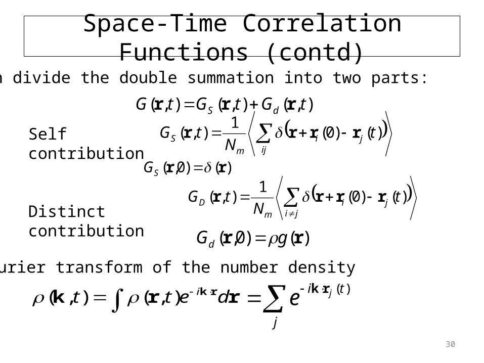
Space-Time Correlation Functions (contd)

),(),(),( tGtGtG dS rrr

ij

jim

S tN

tG )()0(1

),( rrrr

)()0,( rr SG

)()0,( rr gGd

rrk rk dett i),(),( j

ti je )(rk

Can divide the double summation into two parts:

Self contribution

Distinct contribution

ji

jim

D tN

tG )()0(1

),( rrrr

Fourier transform of the number density

31

Space-Time Correlation Functions (contd.)

rrk rk detGtF ),(),(

)0,(),(1

kk tNm

dtetFS t

),(

2

1),( kk

)(),( kk SdS

)0,()( kk FS

Intermediate scattering function

Static structure factor

Dynamic structure factor

Sum rule

32

References• D. Frenkel and B. Smit, Understanding Molecular

Simulations: From Algorithms to Applications• D. C. Rapaport, The Art of Molecular Dynamics

Simulation (Details of how to implement algorithms for molecular systems)

• M. P. Allen and D. J. Tildesley, Computer Simulation of Liquids (SHAKE, RATTLE, Ewald subroutines)

• Haile, Molecular Dynamics Simulation: Elementary Methods

• D. Chandler, Introduction to Modern Statistical Mechanics (Linear Response Theory)

• D. A. McQuarrie, Statistical Mechanics (Spectroscopic Properties)

• J.-P. Hansen and I. R. McDonald, The Theory of Simple Liquids (Almost everything)