1

Robert EngleUCSD and NYU

July 2000

2

WHAT IS LIQUIDITY?

A market with low “transaction costs” including execution price, uncertainty and speed

This may mean different things depending upon the volume to be traded and impatience of the trader.

3

THREE MEASURES:

Bid Ask Spread– measures costs for small trades

Depth– quoted depth for small trades– depth with some price deterioration

Price Impact of a Trade– how much prices move in response to a

large trade

4

BUY VOLUMESELL VOLUME

PRICE

BID ASKSPREAD

MARKETDEPTH

SLOPEIS PRICEIMPACT

5

HOW DO THESE MEASURES OF LIQUIDITY VARY OVER TIME AND CAN THEY BE PREDICTED? BRIEFLY -THE ANSWER FIRST!! ACROSS ASSETS – MORE

TRANSACTIONS AND MORE VOLUME MEANS MORE LIQUIDITY.

HOWEVER – OVER TIME, MARKETS BECOME LESS LIQUID WHEN THEY ARE MORE ACTIVE!!!

6

WHY SHOULD EXECUTION BE WORSE WHEN THE MARKET IS ACTIVE?

Because the market is more active when there is information flowing.

When there is information, traders watch trades (and each other) to learn the information as quickly as possible

Often called “Price Discovery”

7

MICROSTRUCTURE THEORY

Inventory models– More trades make inventories easier to

manage– lower transaction costs and more liquidity

Asymmetric Information models– More informed traders increase adverse

selection costs - greater spreads and price impacts

8

ASYMMETRIC INFORMATION MODELS Glosten and Milgrom(1985) following

Bagehot(1971) and Copeland and Galai(1983)

A fraction of the traders have superior information about the value of the asset but they are otherwise indistinguishable.

9

MARKET MAKER INFERENCE PROBLEM: If the next trader is a buyer, this raises

my probability that the news is good. Knowing all the probabilities I can calculate bid and ask prices:

Over time, the specialist and the market ultimately learn the information and prices reflect this.

askPnewbuyhistorypastValueE )(

10

Easley and O’Hara(1992)

Three possible events- Good news, Bad news and no news

Three possible actions by traders- Buy, Sell, No Trade

Same updating strategy is used

11

BEGINNING OF DAY

P(INFORMATION)=P(GOOD NEWS)=

P(AGENT IS INFORMED)=P(UNINFORMED WILL BE BUYER)=

P(UNINFORMED WILL TRADE)=

END OF DAY

12

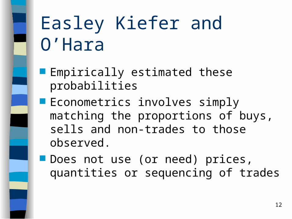
Easley Kiefer and O’Hara

Empirically estimated these probabilities Econometrics involves simply matching

the proportions of buys, sells and non-trades to those observed.

Does not use (or need) prices, quantities or sequencing of trades

13

49.9

50.0

50.1

50.2

50.3

10 20 30 40 50 60 70 80 90 100

EVA EVB

14

49.9

50.0

50.1

50.2

50.3

10 20 30 40 50 60 70 80 90 100

EVA EVB

15

50.00

50.05

50.10

50.15

50.20

50.25

50.30

2 4 6 8 10 12 14

ASK1ASK_EKO

ASK2ASK3

ASK4

ASKING QUOTES WITH VARIOUS FRACTIONSOF INFORMED TRADERS

16

50.00

50.05

50.10

50.15

50.20

50.25

50.30

2 4 6 8 10 12 14

EVAEVANEVA2N

EVA3NEVA4NEVA5N

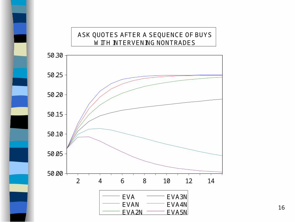
ASK QUOTES AFTER A SEQUENCE OF BUYSWITH INTERVENING NONTRADES

17

LIQUIDITY IMPLICATIONS

When the proportion of informed traders is high, the market is less liquid in all dimensions

When information flows, there are more informed traders, as they rush to trade ahead of price movements

For specific public news events, this could approach 100%

18

INFORMED TRADERS

What is an informed trader? – Information about true value– Information about fundamentals– Information about quantities– Information about who is informed

19

PRICE IMPACTS OF TRADES

In real settings where traders have a choice about when to trade, how to trade and how much to trade– Their choices may indicate whether they

have information– Large trades and rapid trades and trades

by big players all have greater price impacts

20

Econometric Tools

Data are irregularly spaced in time The timing of trades is informative Need to model jointly the time and

characteristics of a trade This is called a marked point process Will use Engle and Russell(1998)

Autoregressive Conditional Duration (ACD)

21

STATISTICAL MODELS

There are two kinds of random variables:– Arrival Times of events such as trades– Characteristics of events called Marks

which further describe the events Let x denote the time between trades

called durations and y be a vector of marks

Data: }N,...1i),y,x{( ii

22

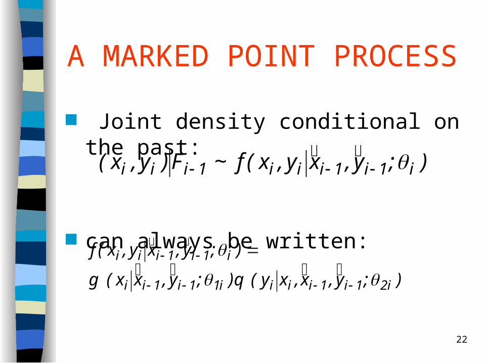
A MARKED POINT PROCESS

Joint density conditional on the past:

can always be written:

);y,xy,x(f~)y,x( i1i1iii1iii

F

);y,x,xy(q);y,xx(g

);y,xy,x(f

i21i1iiii11i1ii

i1i1iii

23

THE CONDITIONAL INTENSITY PROCESS The conditional intensity is the

probability of an event at time t+t given past arrival times and the number of events.( , ( ); ,..., )

( ( ) ( ) ( ), ,..., )

( )

( )lim

t N t t t

P N t t N t N t t t

t

N t

t

N t

1

0

1

24

THE ACD MODEL

The statistical specification is:

where is the conditional duration and is an i.i.d. random variable with non-negative support

(i)

i i i i it t E x t t ( , ..., ; ) [ , ..., ]1 1 1 1

(ii) xi i i

25

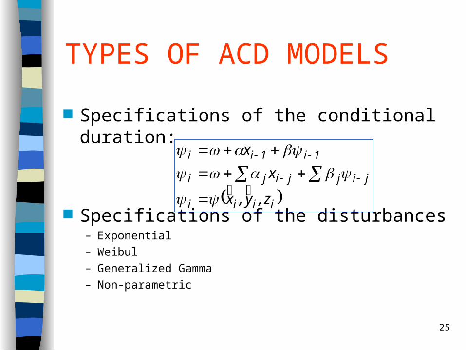
TYPES OF ACD MODELS

Specifications of the conditional duration:

Specifications of the disturbances– Exponential

– Weibul

– Generalized Gamma

– Non-parametric

iiii

jijjiji

1i1ii

z,y,x

x

x

26

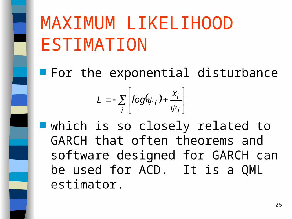
MAXIMUM LIKELIHOOD ESTIMATION For the exponential disturbance

which is so closely related to GARCH that often theorems and software designed for GARCH can be used for ACD. It is a QML estimator.

i i

ii

xlogL

27

EMPIRICAL EVIDENCE

Dufour and Engle(2000), “Time and the Price Impact of a Trade”, Journal of Finance, forthcoming

Engle, Robert and Jeff Russell,(1998) “Autoregressive Conditional Duration: A New Model for Irregularly Spaced Data, Econometrica

Engle, Robert,(2000), “The Econometrics of Ultra-High Frequency Data”, Econometrica

Engle and Lunde, “Trades and Quotes - A Bivariate Point Process”

Russell and Engle, “Econometric analysis of discrete-valued,

irregularly-spaced, financial transactions data”

28

29

APPROACH

Extend Hasbrouck’s Vector Autoregressive measurement of price impact of trades

Measure effect of time between trades on price impact

Use ACD to model stochastic process of trade arrivals

30

DATA:

TORQ dataset -transactions on 18 stocks for 3 months from Nov. 1990-Jan 1991. These are the actively traded stocks.

31

DEFINITIONS

PRICE is midquote when a trade arrives(actually use 5 seconds before a

trade).

R is the log change in PRICE

T is the time between transactions

X = 1 if transaction price> midquote, i.e. BUY

X= -1 if transaction price < midquote, SELL

X= 0 if transaction price = midquote

V is the number of shares in a transaction

32

CORRELATIONS

[ABS(R), T(-1)] <0, FOR 16

[SPREAD, T(-1) ]< 0, FOR ALL 18

[ABS(R), V(-1)] >0 , FOR ALL 18

33

HASBROUCK MODEL (1991)GENERALIZED FOR TIME EFFECT

Vector Autoregression of trade directions and returns

Use to calculate the long run effect of trades on prices as a function of time between trades

.vx ))Tln((xDrcx

vx ))Tln((xDrar

t,2

5

1iitit

xi

xi1t1t

xopen

5

1iitit

t,1

5

0iitit

ri

ritt

ropen

5

1iitit

34

RESULTS FOR RETURN EQUATION: o > 0 for all 18, all very significant

– Buys raise prices o < 0 for 17, 13 significant

– Buys raise prices more when durations are short H: all = 0; rejected for 13

– Time Matters H: ;

• rejected for 13,• negative for 16

05

1i

ri

35

for 18 , all very significant,

– serial correlation in trade direction for 15, significantly negative for 10,

– short durations increase autocorrelation rejected for 11

rejected for 12, 11 negative– time matters for trade dynamics

x5

x10 ...0:H

0:H5

1i

xi0

0x1

0x1

RESULTS FOR TRADE EQN.

36

INTRODUCING OTHER INTERACTIONS

H: all =0; rejected for 8 of 18 stocks. Volume and Spread are very significant

iti,3i,2iti,1iit

t

5

0iitittopen

5

1iitit

Sprd)Vln()Tlog(b

XbDRR

37

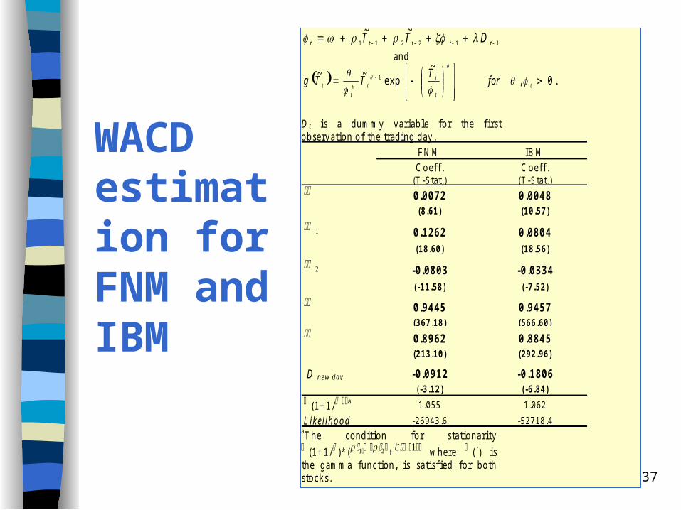
WACD estimation for FNM and IBM

112211

~~ ttttt DTT

a n d

.0, ~

exp~~ 1

t

t

tt

t

t forT

TTg

D t i s a d u m m y v a r ia b le fo r th e f i r s to b s e rv a t io n o f th e t r a d in g d a y .

F N M IB M

C o e f f . C o e f f .( T - S t a t . ) ( T - S t a t . )

0 .0 0 7 2 0 .0 0 4 8( 8 .6 1 ) ( 1 0 .5 7 )

0 .1 2 6 2 0 .0 8 0 4( 1 8 .6 0 ) ( 1 8 .5 6 )

-0 .0 8 0 3 -0 .0 3 3 4( - 1 1 .5 8 ) ( - 7 .5 2 )

0 .9 4 4 5 0 .9 4 5 7( 3 6 7 .1 8 ) ( 5 6 6 .6 0 )

0 .8 9 6 2 0 .8 8 4 5( 2 1 3 .1 0 ) ( 2 9 2 .9 6 )

D n e w d a y -0 .0 9 1 2 -0 .1 8 0 6( - 3 .1 2 ) ( - 6 .8 4 )

(1 + 1 / a 1 .0 5 5 1 .0 6 2

L ik e lih o o d - 2 6 9 4 3 .6 - 5 2 7 1 8 .4a T h e c o n d i t io n fo r s ta t io n a r i ty (1 + 1 / )* ( + w h e re () i sth e g a m m a fu n c t io n , i s s a t i s f ie d fo r b o ths to c k s .

38

CALCULATE IMPULSE RESPONSES OF A TRADE. WITH DURATIONS FIXED AT A

PARTICULAR VALUE WITH DURATIONS EVOLVING

JOINTLY MEASURED IN CALENDAR TIME

RATHER THAN TRANSACTION TIME Latter two require stochastic simulation

of the ACD

39

Cumulative percentage quote revision after an

unexpected buy

0

0.02

0.04

0.06

0.08

1 3 5 7 9 11 13 15 17 19 21

1/17/91

12/24/90

Transaction Time (t)

40

Cumulative percentage quote revision after an unexpected buy

0

0 .02

0 .04

0 .06

0 .080

:00

02:0

5

04:1

0

06:1

5

08:2

0

10:2

5

12:3

0

14:3

5

16:4

0

18:4

5

20:

50

Calendar time (min:sec)

1/17/91

12/24/90

41

SUMMARY The price impacts, the spreads, the

speed of quote revisions, and the volatility all respond to information

Econometric measures of information – high shares per trade– short duration between trades– wide spreads

42

CONCLUSIONS

MARKETS ARE LESS LIQUID WHEN THEY ARE MORE ACTIVE

TRANSITION TO FULL INFORMATION OR EFFICIENT PRICES IS FASTER WHEN THERE IS INFORMATION ARRIVING