1 predicting and understanding the breakdown of linear flow models p. stuart, i. hunter, r....
TRANSCRIPT

1
Predicting and Understanding the Breakdown of Linear Flow Models
P. Stuart, I. Hunter, R. Chevallaz-Perrier, G. Habenicht
19 March 2009
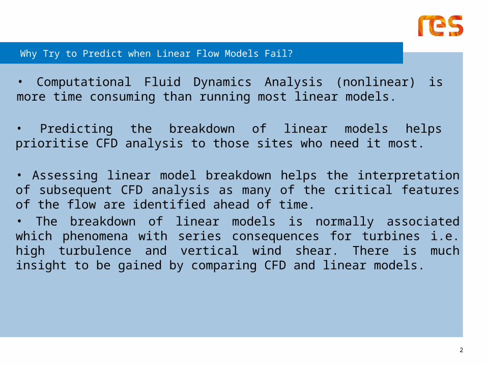
Why Try to Predict when Linear Flow Models Fail?
2
• Computational Fluid Dynamics Analysis (nonlinear) is more time consuming than running most linear models.
• Predicting the breakdown of linear models helps prioritise CFD analysis to those sites who need it most.
• Assessing linear model breakdown helps the interpretation of subsequent CFD analysis as many of the critical features of the flow are identified ahead of time.
• The breakdown of linear models is normally associated which phenomena with series consequences for turbines i.e. high turbulence and vertical wind shear. There is much insight to be gained by comparing CFD and linear models.

3
What is a Linear Hill?
If the wind flow over a hill can be assumed to be linear then the effects of a single hill can be decomposed into several smaller hills.
= +
Another example:
=h
L
One example:
+L
0.5h
Models like WASP / MS3DJH decompose real terrain into many sinusoidal hills, solve them individually and then recombine to get their final solution.

4
Why does linear theory break down?
The linear theory (from which both WASP and MS3DJH are derived) simplifies the governing flow equations under the assumption of small terrain slope.
),,()(),,( 0 zyxuzuzyxu 0
*0 ln)(
z
zuzu
),,(ˆ),,( * zyxuuzyxu (Jackson and Hunt, 1975)
The velocity is decomposed as follows:
• is assumed to be O(1).• ε is assumed to be small.• Linearise by neglecting terms O(ε2).• ε increases with increasing slope.• For large slopes ε becomes large and the theory becomes invalid.
u
perturbationundisturbed

Methodology
• Calculate flow over idealised hills using both CFD and linear models for incrementally increasing slopes and tree heights.
MS3DJH / RES Roughness
• Establish guidelines for where linear models fail by comparing to CFD.
Linear CFD
• Use simple geometrical considerations to assess likely impact on real sites.
• Confirm predicted effects using CFD.

Computer code
Mathematical and Physical Modelling
• Reynolds averaged Navier Stokes (RaNS) equations
• Two-equation (k-ε) turbulence model with canopy model
• Terrain-following coordinate system
Numerical Techniques
• Finite volume
• SIMPLE algorithm
• Steady State & Transient

7
Breakdown of Linear Behaviour for a 2D Symmetric Hill
16°
RecirculationAttached Boundary Layer
<10% Difference between Linear and
CFD
>10% Difference between Linear and
CFD

3D Symmetric: Max Slope 16°3D Symmetric: Max Slope 21°
8
Comparison of 2D and 3D Symmetric Hills
2D Symmetric: Max Slope 16°
c.f. Kaimal and Finnigan (1994): 2D Critical slope ~18°, 3D Critical Slope ~20°.
9
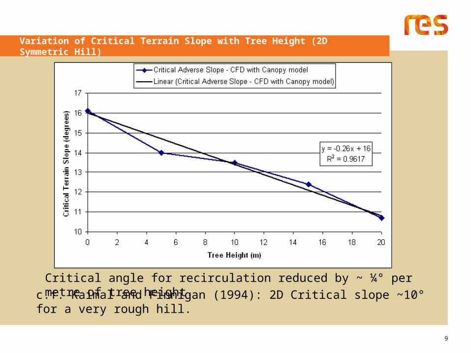
Variation of Critical Terrain Slope with Tree Height (2D Symmetric Hill)
Critical angle for recirculation reduced by ~ ¼° per metre of tree height.
c.f. Kaimal and Finnigan (1994): 2D Critical slope ~10° for a very rough hill.

Variation of Critical Terrain Slope with Tree Height (2D Symmetric Hill)
Critical angle for linear model break down reduced by ~½° per metre of tree height.
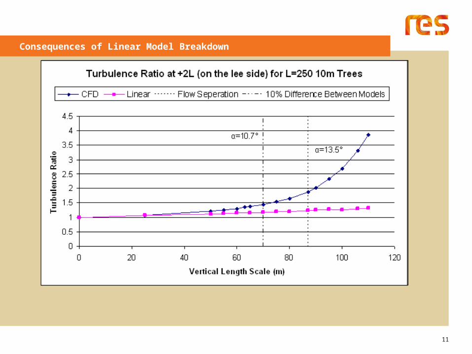
Consequences of Linear Model Breakdown
11

Case Study #1 : Complex Terrain Short Trees
12
β
Predominant wind direction
• Plot adverse gradients exceeding threshold by direction.
dy
dh)180cos(+
dx
dh)180sin(tan= 1-
• Identify turbines downwind of critical adverse gradients.
•Consider spreading of terrain induced wake (β~5°).
• Establish critical angle considering tree height (3m).
154
16= TR
H 5.142
16= TN
H
β

Case Study #2 : Complex Terrain No Trees
13
β
Predominant wind direction
• No trees, critical angle: φR=φN=16°
Transient CFD: Turbulence

Case Study #3 : Complex Terrain With Tall Trees
14
• Establish critical angles considering tree height (20m).
114
16= TR
H 62
16= TN
H
Predominant wind direction

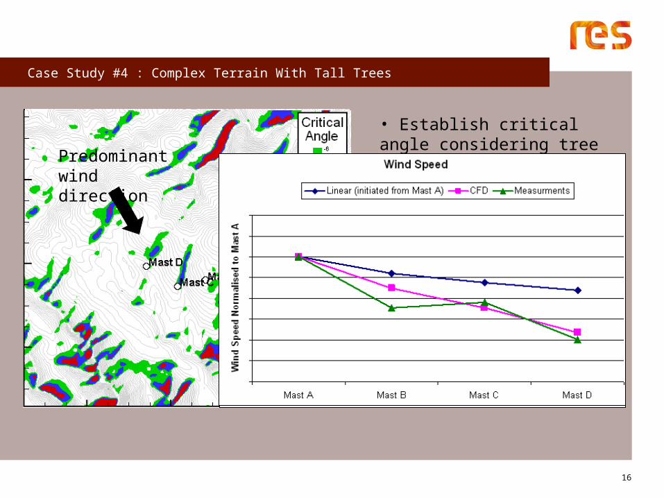
Case Study #4 : Complex Terrain With Tall Trees
Case Study #4 : Complex Terrain With Tall Trees
16
• Establish critical angle considering tree height (20m).
114
16= TR
H 62
16= TN
HPredominant wind direction

17
Conclusions
• Considering the critical angle and using simple geometry can provide an extremely useful insight into where linear models are likely to fail. This helps identify where it is necessary to apply CFD.
• CFD indicates critical angle for recirculation is reduced by around ¼° per metre of tree height.
• Terrain assessment method can produce false positives, but CFD analysis provides clarification.
• CFD indicates critical angle for linear model breakdown is reduced by around ½° per metre of tree height.
• Comparison with measurements demonstrates the value of the analysis.
•This presentation summarises 7 to 8 years of experience of learning how to take advantage of CFD modelling within RES

18