1: Photometry

The mathematical thermology created by Fourier may tempt us to hope that. . . wemay in time ascertain the mean temperature of the heavenly bodies: but I regardthis order of facts as forever excluded from our recognition.

Auguste Comte Cours de la Philosophie Positive1 (1835)

. . . within a comparatively few years, a new branch of astronomy has arisenwhich studies the sun, moon, and stars for what they are in themselves and inrelation to ourselves.

Samuel Pierpont Langley The New Astronomy (1888)

Purpose

In 1835 the French philosopher Auguste Comte noted that since we know stars only bytheir light (and cannot take bits of stars into the laboratory), our knowledge of stars wouldbe forever limited essentially to location. Fifty years later astrophysics—the study of thephysics of stars—was beginning, and the first measurements of the Sun’s temperature andcomposition were being made. Evidently, careful measurement of starlight (photometry)allows the intrinsic properties of stars to be determined. In this lab you will use broadbandphotometry to measure the temperature of stars.

Introduction

We begin our study of stars with blackbody radiation, which you studied in Modern Physicsand you will yourself measure in the Thermionic Emission lab (p. 113). The light producedby a hot object is akin to audio noise: in both cases a random process produces a simul-taneous superposition of a wide distribution of wavelengths. In his Opticks, Newton notedcertain systematic dependencies in the light emitted by incandescent objects and suggestedsomething fundamental was behind the process2. Apparently the light produced by an in-candescent object is fundamentally related to its temperature not its material composition.In 1879 Joseph Stefan proposed that every object emits light energy at the rate (power in

1http://socserv2.mcmaster.ca/~econ/ugcm/3ll3/comte/ provides this as an etext translated andedited by Harriet Martineau.

2Query 8: Do not all fix’d Bodies, when heated beyond a certain degree, emit Light and shine. . .Query 11:. . . And are not the Sun and fix’d Stars great Earths vehemently hot. . .

21

22 Photometry

watts):P = ǫT σT 4A (1.1)

where σ is the Stefan-Boltzmann3 constant, T is the temperature of the body, A is thesurface area of the body, and ǫT is the total emissivity.

Experimentally it was found that the wavelength distribution of the light from hot objectswas broadly similar to the Maxwell-Boltzmann speed distribution: a bell-shaped curve inwhich the location of the peak depended on temperature. In 1893 Wilhelm Wien4 concludedthat the wavelength of this peak must be inversely proportional to temperature. Experimentconfirmed that the wavelength of this peak was given by:

λmax =2898 µm · K

T(1.2)

Together the Stefan-Boltzmann and Wien displacement laws—both the results of classicalphysics—explain much of what is commonly observed in hot objects. At room tempera-ture objects do not appear to be a source of light: they appear dark (unless externallyilluminated). This is a result both of the small rate of emission given by Stefan-Boltzmannand (from Wien) for T = 300 K, we find λmax ∼ 10 µm, that is the wavelengths typicallyemitted are well outside the range of light that can be detected by the eye5. On the otherhand for an object like the Sun: T ≈ 6000 K, so λmax ∼ 0.5 µm — right in the middle ofof the visible range.

Our ‘spherical cow’ model6 of a star is an incandescent ball (radius R) of gas shining as ablackbody. Thus the total power output of a star (called the luminosity7) is

L = σT 4 4πR2 (1.3)

The equation for the exact distribution of photon wavelengths produced by a blackbodywas actively researched with erroneous equations produced by Wien and Rayleigh & Jeans.In 1900 Max Planck8 published his derivation of the wavelength distribution of light froma blackbody. However before we can discuss his result we must explain what precisely ismeant by ‘wavelength distribution’.

In Physics 211 you learned about the speed distribution9 of the molecules in a gas: abell-shaped curve that shows that slow molecules are rare and supersonic molecules are

3In 1879 Jozef Stefan (1835–93) proposed the law based on experimental measurements; five years laterLudwig Boltzmann (1844–1906) derived the result from fundamental thermodynamics. Today the result isknown as the Stefan-Boltzmann Law.

4Wilhelm Wien (1864–1928) German physicist, 1911 Nobel Prize in Physics5The human eye can detect light with a wavelength in the range 0.4 µm (violet) to 0.7 µm (red).6This model of a star works best with stars similar in temperature to the Sun, but every star’s light is

considerably modified by absorption as it travels through the star’s atmosphere. In hot stars, UV wavelengthsthat can photoionize hydrogen (H(n = 2)+γ → H++e−) are highly attenuated producing the Balmer jump.The spectra of cool stars shows broad absorption bands due to molecules.http://www.jb.man.ac.uk/distance/life/sample/java/spectype/specplot.htm is an applet allowing acomparison of blackbody light to actual star light.

7The MKS unit for luminosity is watt, but the numbers are so large that it is usually expressed as amultiple (or fraction) of the Sun’s luminosity (a.k.a., solar luminosity) L⊙ = 3.846 × 1026 W.

8Max Planck (1858–1947) German physicist, 1918 Nobel Prize in Physics9Derived by James Clerk Maxwell (1831–1879); Ludwig Boltzmann (1844–1906) provided a firm founda-

tion for the result using statistical mechanics. Today the result is generally known as the Maxwell-Boltzmanndistribution.

Photometry 23

0 .5 1.0 1.5 2.0

10.E+07

8.E+07

6.E+07

4.E+07

2.E+07

0

Blackbody Thermal Radiation

wavelength ( m)

F (

W/m

m

)

6000 K

4000 K

µ

µλ

2

Figure 1.1: The distribution of the light emitted by a blackbody plotted as a function ofwavelength. Hotter objects emit much more light than cool ones, particularly at the shorterwavelengths.

rare, whereas a molecular kinetic energy near 3

2kT is common. ‘Speed probability’ is a

problematic concept. For example the probability that a molecule has a speed of exactlyπ m/s (or any other real number) must be essentially zero10 (as an infinite number of digitsmust match, but there are only a finite [but huge] number of molecules). Probability densityprovides a meaningful context to talk about speed distribution: determine the fraction ofmolecules (‘hits’) that have speed in an interval (bin) (v−∆v/2, v+∆v/2) for various speedsv. (Here the bin is centered on the speed v and has bin-size ∆v.) Clearly the number ofhits in a bin depends on the bin-size (or range), but you should expect that the hit density

(number of hits divided by the bin-size) should be approximately independent of the bin-size. A plot of fraction-per-bin-size vs. bin center provides the usual bell-shaped curve.Bins centered on both slow and supersonic speeds include few molecules whereas bins thatcorrespond to molecular kinetic energy near 3

2kT include a large fraction of molecules.

In a similar way we can sort the light by wavelength into a sequence of wavelength intervals(bins), and calculate the total light energy per bin-size. For example, if there were11 a totalof 2 J of light energy (about 5×1018 photons) with wavelengths in the interval (.50, .51) µmwe would say the intensity of light at λ = .505 µm was about 200 J/µm. In the case ofthe thermal radiation continuously emitted from the surface of a body, we are interested inthe rate of energy emission per area of the body, with units (W/m2)/µm. This quantity iscalled the monochromatic flux density and denoted Fλ

12. Planck’s result was:

Fλ =2πhc2

λ5

1

exp(hc/λkT ) − 1(1.4)

10A mathematician would say the probability is zero for almost every speed.11These numbers correspond approximately to 0.1 sec of full sunlight on 1 m2 of the Earth.12One could just as well measure bin-size in Hz. The result is denoted Fν with units (W/m2)/Hz. A

helpfully sized unit for Fν is the jansky: 1 Jy = 10−26W · m−2· Hz−1. Fν is commonly used in radio

astronomy whereas Fλ is commonly used in optical astronomy.

24 Photometry

where h is Planck’s constant, whose presence is a sign of the importance of quantum me-chanical effects. The primary assumption in Planck’s derivation of this distribution was thephoton: an indivisible packet of light carrying total energy E = hc/λ. With this identifica-tion notice the Boltzmann factor in Planck’s equation: exp(E/kT ). As before, this factormeans that high energy (i.e., short wavelength) photons are rarely in the mix of emittedphotons. Thus only ‘high’ temperature stars will emit an abundance of UV radiation.

Of course, the light emitted from the surface of a star gets spread over an ever larger areaas it moves away from the star. Thus the flux coming into a telescope a distance r from thecenter of the star would be:

Fλ =2πhc2

λ5

R2

r2

1

exp(hc/λkT ) − 1(1.5)

Theoretically its now easy to measure the temperature of stars: simply measure the wave-length distribution (‘spectra’) of the starlight and fit the measurements to the above theorywith two adjustable parameters: T and R/r. (Do notice that increasing R or decreasingr produces exactly the same effect—an overall increase in the flux density—so we cannotseparately determine R and r from the spectra. A large, distant T = 6000 K star couldhave exactly the same spectra as a small, close T = 6000 K star.) Let me enumerate a few(of the many) reasons this does not work perfectly.

1. We assumed above that space was transparent: that the only effect of distance wasdiluting the light over a greater area. However, our Galaxy is filled with patchy cloudsof dust. Unfortunately the dust in these clouds has the property of being more likelyto absorb blue light than red. Thus a dust-obscured star will lose more blue than redlight and the observed spectra will be distorted from that emitted. A dust-obscuredstar would measure cooler and appear more distant (i.e., dimmer) than it actuallywas. These two effects of dust are called ‘reddening’ and ‘extinction’. Of coursesubstantial dust absorption is more likely for more distant stars. It is usually ‘small’for stars within 300 Ly of Earth. However, 300 Ly covers a very tiny fraction ofour Galaxy. In this lab we will side step this problem by selecting stars with littledust absorption. However, with a bit of additional work, dust absorption could bemeasured and corrected for using photometry.

2. Starlight measured from the surface of the Earth must traverse the Earth’s atmo-sphere. The non-transparency of the Earth’s atmosphere will also modify the observedstarlight. In addition, the telescope and detector typically introduce additional ‘non-transparency’, that is blue and red photons at the telescope aperture are not equallylikely to be counted. The ‘efficiency’ of the system depends on wavelength. Unlessextraordinary care is taken, this efficiency can change on a daily basis. (And, ofcourse, the atmosphere’s transparency can change in a matter of minutes.) As a re-sult frequent calibration of the system is required. Calibration at the multitude ofwavelengths required to make a full spectra is obviously more difficult than calibrationat just a few wavelengths.

3. There is a competition between the accurate measurement of the value of Fλ andthe bin-size used. As you should notice in the Bubble Chamber lab, if you select asmall bin-size, each bin captures relatively few hits which results in relatively large√

N errors. So if you have only a few thousand photons, you may do better to usea big bin-size (so you capture enough counts to get an accurate measurement of Fλ),

Photometry 25

but then only have a few bins (each spanning a large interval of in wavelength) so,unfortunately, the spectrum has been reduced to just a few points. Of course, youcould always collect starlight for a longer period of time (longer ‘integration time’)or use a telescope with a larger aperture. However, these solutions miss the point:The boundary between the known and unknown in astronomy is almost always atthe edge of what you can just barely detect. Thus you must always come up withthe maximally efficient use of the available photons. Telescope time is allocated fora detailed spectra only when it is expected that the results cannot be obtained in a‘cheaper’ way.

4. Stars are not exact blackbodies, and of course they are not at a temperature. Cer-tainly if we move from the surface to core of a star we would experience quite differenttemperatures. But even on the ‘surface’ of our Sun we see regions (‘sunspots’) withunusually low temperature. In the Langmuir Probe lab, you will find that the elec-trons in a tube of gas may have a different temperature from the co-mingled atoms.Similarly, in the atmospheres of stars it is not unusual for the various components ofthe gas to be at different temperatures (that is to say the gas is not in local thermody-namic equilibrium [LTE]). Hence it may make no sense to try to obtain high-precisionmeasurements of ‘the’ temperature.

Oddly enough the fact that stars are not blackbodies is actually helpful as it allowsa variety of information to be decoded from the starlight. (A blackbody spectraincludes just two bit of information the temperature T and R/r.) Varying absorptionin the star’s atmosphere means that some light (i.e., λ at which the star’s atmosphereis largely transparent) comes from deeper in the star and hence represents a highertemperature. Ultimately the absorption lines in a star’s spectra provide the bulk ofthe information we have about stars. Chemical composition of the star’s atmosphereand temperature—accurate13 to a few percent—are best obtained this way. However,consideration of these absorption lines is beyond the aims of this lab.

Temperature I

Our aim in this lab is to measure the temperature of stars without resorting to a detailedmeasurement of the star’s spectra. We begin by considering measurement of Fλ at just twowavelengths: F1 at λ1 and F2 at λ2 where λ1 < λ2. (Think of λ1 as blue light and λ2 asred light.) There is a huge cancellation of factors if we look at the ratio: F2/F1:

F2

F1

=λ5

1

λ52

exp(hc/λ1kT ) − 1

exp(hc/λ2kT ) − 1(1.6)

In general, ratios are great things to measure because (A) since they are dimensionless theyare more likely to be connected to intrinsic properties and (B) it is often the case thatsystematic measurement errors will (at least in part) cancel out in a ratio.

While the ratio has considerably reduced the complexity of the formula, it would help ifwe had an even simpler formula. Towards that goal we make the approximation that the

13Statements like this—that imply we know the true accuracy of our measurements—should be read withthe knowledge that history shows unexpected jumps in measurements as systematic errors are discovered.The history of the measured chemical composition of stars would show graphs much like those in Figure 1on page 10.

26 Photometry

exponential terms are much larger than 1:

F2

F1

=λ5

1

λ52

exp(hc/λ1kT ) − 1

exp(hc/λ2kT ) − 1(1.7)

≈ λ51

λ52

exp(hc/λ1kT )

exp(hc/λ2kT )=

λ51

λ52

exp

[

hc

kT

(

1

λ1

− 1

λ2

)]

(1.8)

log(F2/F1) ≈ hc

kT

(

1

λ1

− 1

λ2

)

log e + 5 log(λ1/λ2) (1.9)

Example

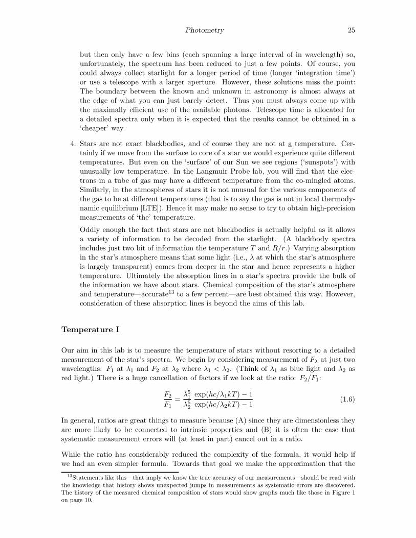
Consider the case where λ1 = .436 µm (blue) and λ2 = .545 µm (yellow or ‘visible’). Forhistorical reasons, astronomers prefer to consider 2.5 log10(F2/F1), and if we evaluate all ofthe constants we find:

2.5 log10(F2/F1) ≈7166 K

T− 1.21 (1.10)

Do notice that for cool stars this quantity is large (more ‘visible’ than blue light) andthat extremely hot stars (T → ∞) will all have much the same value for this quantity:−1.21. This last result is a consequence of the ‘Rayleigh-Jeans’ approximation for thePlanck distribution, valid for λ ≫ λmax. In this large wavelength (or high temperature)limit, the Boltzmann factors are nearly one and:

exp(hc/λkT ) − 1 ≈ hc/λkT (1.11)

so14

Fλ ≈ 2πhc2

λ5

λkT

hc= kT

2πc

λ4(1.12)

Since temperature is now an over-all factor, it will cancel out in any flux ratio.

Color Index

At increasing distance from the star, both F2 and F1 will be diminished, but by exactly thesame fraction (assuming space is transparent, or at least not colored). Thus this ratio is anintrinsic property of the star, and you saw above that this ratio is related to the temperatureof the star. The ratio is, of course, a measure of the relative amounts of two colors, and assuch is called a color index. (Our experience of color is independent of both the brightnessof the object and the distance to the object. It instead involves the relative amounts of theprimary colors; hence the name for this ratio.) Any two wavelengths λ1, λ2 can be used toform such a color index, but clearly one should select wavelengths at which the stars arebright and λ . λmax (to avoid the Rayleigh-Jeans region where the ratio is independent oftemperature).

Magnitude

For historical reasons, astronomers typically measure light in magnitudes. Magnitudes arerelated to fluxes by:

m = −2.5 log10(F/F0) (1.13)

14Do notice the absence of h in this classical result.

Photometry 27

2000 4000 8000 20,000 40,000

2

1

0

–1

Color Index vs. Temperature

Temperature (K)

Col

or I

ndex

Figure 1.2: In the case where λ1 = .436 µm (blue) and λ2 = .545 µm (yellow or ‘visible’), the‘color index’ 2.5 log(F2/F1) is plotted as a function of temperature. The dotted line showsthe approximate result Eq. 1.10; the solid line shows the actual ratio of Planck functions.Do remember that high temperature stars have a smaller, even negative, color index.

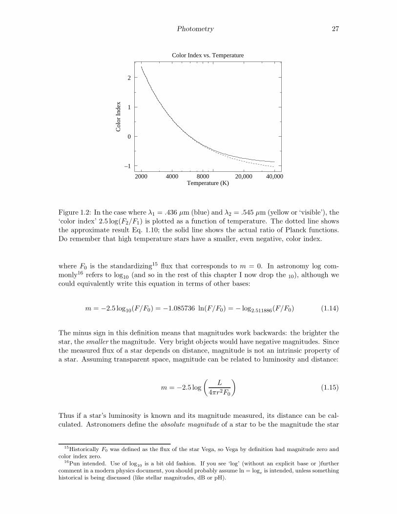
where F0 is the standardizing15 flux that corresponds to m = 0. In astronomy log com-monly16 refers to log10 (and so in the rest of this chapter I now drop the 10), although wecould equivalently write this equation in terms of other bases:

m = −2.5 log10(F/F0) = −1.085736 ln(F/F0) = − log2.511886(F/F0) (1.14)

The minus sign in this definition means that magnitudes work backwards: the brighter thestar, the smaller the magnitude. Very bright objects would have negative magnitudes. Sincethe measured flux of a star depends on distance, magnitude is not an intrinsic property ofa star. Assuming transparent space, magnitude can be related to luminosity and distance:

m = −2.5 log

(

L

4πr2F0

)

(1.15)

Thus if a star’s luminosity is known and its magnitude measured, its distance can be cal-culated. Astronomers define the absolute magnitude of a star to be the magnitude the star

15Historically F0 was defined as the flux of the star Vega, so Vega by definition had magnitude zero andcolor index zero.

16Pun intended. Use of log10 is a bit old fashion. If you see ‘log’ (without an explicit base or )furthercomment in a modern physics document, you should probably assume ln = log

eis intended, unless something

historical is being discussed (like stellar magnitudes, dB or pH).

28 Photometry

would have if observed from a distance of 10 pc17. Thus:

m = −2.5 log

[

L

4πr2F0

]

(1.16)

= −2.5 log

[

(

L

4π(10 pc)2F0

)

·(

10 pc

r

)2]

(1.17)

= −2.5 log

[

L

4π(10 pc)2F0

]

+ 5 log

[

r

10 pc

]

(1.18)

= M + 5 log

[

r

10 pc

]

(1.19)

where M is the absolute magnitude and the remaining term: 5 log(r/10 pc) is known as thedistance modulus. The main point here is that distance affects magnitude as a constantoffset. This result is a lemma of the general result:

Theorem: If the measured flux Fm is a fraction (ǫ) of the actual flux F (as wouldoccur due to a less-than-perfectly efficient detector, a dusty mirror, atmospheric absorption,absorption due to interstellar dust,. . . ) the resulting magnitude as measured (mm) is justa constant (2.5 log ǫ) off from the actual magnitude (m).

Proof:

mm = −2.5 log(Fm/F0) (1.20)

= −2.5 log(ǫF/F0) (1.21)

= −2.5 log(F/F0) − 2.5 log(ǫ) (1.22)

= m − 2.5 log(ǫ) (1.23)

Much of this lab will involve finding the constant offset that relates our measured (instru-mental) magnitudes to the actual (standardized) magnitude.

Filters

In the above equation for magnitude, the flux might be the total (all wavelengths or ‘bolo-metric’) light flux, or a monochromatic flux density Fλ, or the flux in a particular rangeof wavelengths. Much of astronomy is concerned with the flux through the five standard18

U , B, V , R, and I filters. The characteristics of these filters are detailed in Figure 1.3,but essentially each filter allows transmission of a range of wavelengths ∆λ, centered ona particular wavelength. The name of the filter reports the type of light allowed to pass:U (ultraviolet), B (blue), V (‘visible’, actually green), R (red), and I (infrared). The fil-ters are broad enough that the resulting bin really doesn’t well represent a value for Fλ.(An appendix to this chapter describes the u′g′r′i′z′ filters19 used in the Sloan Digital SkySurvey.)

The magnitude of a star as measured through a B filter is called the B magnitude andis simply denoted: B. Notice that we can now form color indices just by subtracting two

17pc = parsec = 3.0857 × 1016 m = 3.2616 Ly18Johnson, H. L. and Morgan, W. W. (1951) ApJ 114 522 & (1953) ApJ 117 313

Cousins, A.W.J. (1976) memRAS 81 2519Fukugita, M., Ichikawa, T., Gunn, J. E., et al. 1996 AJ, 111, 1748

Photometry 29

.4 .6 .8 1.0 1.2

1.0

.8

.6

.4

.2

0

Johnson–Cousins UBVRI

Tra

nsm

issi

on

wavelength ( m)

U B V R I

µ

Filter λ ∆λ F0

Name (µm) (µm) (W/m2 µm)

U 0.36 0.07 4.22 × 10−8

B 0.44 0.10 6.40 × 10−8

V 0.55 0.09 3.75 × 10−8

R 0.71 0.22 1.75 × 10−8

I 0.97 0.24 0.84 × 10−8

Figure 1.3: The characteristics of the standard filters: U (ultraviolet), B (blue), V (visible),R (red), I (infrared) from Allen’s Astrophysical Quantities p. 387 and The General Catalogueof Photometric Data: http://obswww.unige.ch/gcpd/system.html

30 Photometry

0 .5 1.0 1.5 2.0

14000

12000

10000

8000

6000

4000

Temperature vs B–V

B–V

Tem

pera

ture

(K

)

0 .5 1.0 1.5 2.0

12000

10000

8000

6000

4000

Temperature vs R–I

R–I

Tem

pera

ture

(K

)

Figure 1.4: Using data from Allen’s Astrophysics Quantities calibration curves relatingstellar temperature to color index can be obtained. The fit equations for these curves isgiven in the text.

magnitudes. For example, the most common color index is B − V :

B − V = 2.5 (log(FV /FV 0) − log(FB/FB0)) (1.24)

= 2.5 (log(FV /FB) + log(FB0/FV 0)) (1.25)

= 2.5 log(FV /FB) + constant (1.26)

So B − V is related to the flux ratio FV /FB and so is an intrinsic property of the starrelated to temperature. Furthermore, while Eq. 1.10 was derived assuming monochromaticflux densities (in contrast to the broad band fluxes that make up B and V ), we can still hopeequations similar to Eq. 1.10 can be derived for B − V . Allen’s Astrophysical Quantities

provides calibration data to which Kirkman has fit a curve:

B − V =35800

T + 3960− 3.67 + 1.08 × 10−4 T (1.27)

and the inverse relationship:

T =1700

(B − V ) + .36+ 5060 − 1600(B − V ) (1.28)

The data with fitted curve is plotted in Figure 1.4. Notice that for B − V < 0 smalluncertainties in B − V result in large uncertainties in T : it would probably we wise toswitch to a different color index like U − B to measure the temperature of such a hot star.

Similar work can be done for R − I, with results:

T =2750

(R − I) + .314+ 1400 + 160(R − I) (1.29)

For the Sun, Allen’s Astrophysics Quantities reports: T=5777 K, B − V =0.65, R− I=0.34whereas Eq. 1.28 gives 5703 K and Eq. 1.29 gives 5659 K. In general errors of a few percentshould be expected.

Photometry 31

Temperature II

The starting point for physics is usually hard intrinsic quantities like temperature, densityand pressure. However, in astronomy the transducers20 used to measure these quantities areparts of the star itself (say the absorption lines of a particular element in the atmosphere ofthe star). We will always be a bit uncertain about the exact situation of these transducers,and hence the calibration of these transducers is correspondingly uncertain. For examplestars with unusual chemical composition (like population II stars) or unusual surface gravityg (like giant stars) really deserve separate calibration curves. Since the usual physicalquantities are in astronomy provisional and subject to recalibration, astronomers attachprimary importance to the quantities that are not subject to the whims of revised theory:the actual measurements of light intensity. Thus astronomers use as much as possiblehard quantities21 like B − V directly without converting them to temperature using someprovisional formula. For example just using B − V , stars can be arranged in temperature-increasing order, since there is a monotone relationship between B − V and T . Of course,in this lab the aim is to measure star temperatures in normal units.

Summary

In this lab you will measure the temperature of stars by measuring their B,V,R, I magni-tudes, calculating the color indices B−V and R−I, and then, using the supplied calibrationcurves, find T . The calibration curves are based on detailed spectra of bright, normal stars;In using these calibration curves we are automatically assuming our (distant and hencedimmer) target stars are also ‘normal’.

Detector System

In this lab photons are counted using a charge coupled device or CCD. Our Kodak KAF-1001E CCD consists of a typical 26-pin DIP integrated circuit with a window that exposes tolight a 1”×1” field of 1024×1024 light sensitive regions or pixels. Photons incident on a pixelfree electrons via the photoelectric effect22. Each pixel stores its charge during an exposure,and then each bucket of charge is transferred (in a manner similar to a bucket brigade)to a capacitor where it produces a voltage proportional to the number of electrons. Ananalog-to-digital converter then converts that voltage to a 16-bit binary number (decimal:

20In normal usage, a transducer is a device which converts a physical quantity (e.g., pressure, temperature,force,. . . ) to an electrical quantity (volts, amps, Hz . . . ) for convenient measurement: for example, amicrophone. Here I’ve broadened the usual meaning to include natural ‘devices’ whose emitted or absorbedlight allows a physical quantity to be determined. Obviously we are connected to the stars by light, notcopper wires.

21In this lab you will see that even as simple a quantity as B is actually only distantly related to directmeter readings. The direct meter readings must be ‘reduced’ to eliminate confounding factors like detectorefficiency or atmospheric absorption. Nevertheless, since these problems are ‘at hand’ astronomers believethat they can be properly treated. Astronomers willing archive B data, whereas T calculations are alwaysconsidered ephemeral.

22Albert Einstein (1879–1955) received the 1921 Nobel prize for his 1905 theory explaining this effect.Robert Millikan’s [(1868–1953), B.A. Oberlin College, Ph.D. Columbia] experimental studies (1912–1915) ofthe photoelectric effect were cited, in part, for his Nobel in 1923.

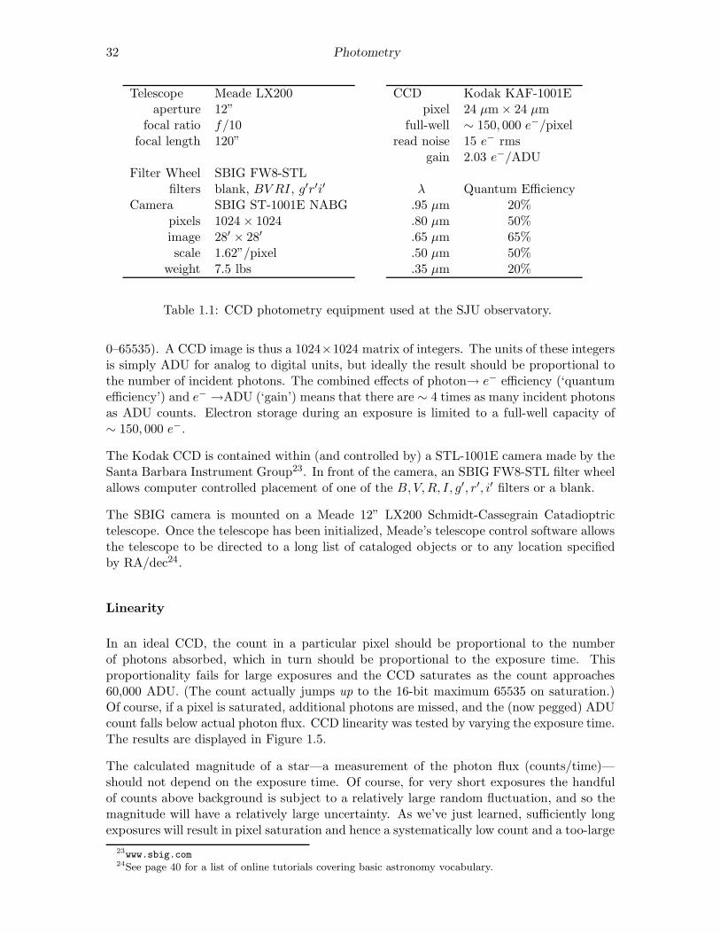
32 Photometry

Telescope Meade LX200aperture 12”

focal ratio f/10focal length 120”

Filter Wheel SBIG FW8-STLfilters blank, BV RI, g′r′i′

Camera SBIG ST-1001E NABGpixels 1024 × 1024image 28′ × 28′

scale 1.62”/pixelweight 7.5 lbs

CCD Kodak KAF-1001Epixel 24 µm × 24 µm

full-well ∼ 150, 000 e−/pixelread noise 15 e− rms

gain 2.03 e−/ADU

λ Quantum Efficiency.95 µm 20%.80 µm 50%.65 µm 65%.50 µm 50%.35 µm 20%

Table 1.1: CCD photometry equipment used at the SJU observatory.

0–65535). A CCD image is thus a 1024×1024 matrix of integers. The units of these integersis simply ADU for analog to digital units, but ideally the result should be proportional tothe number of incident photons. The combined effects of photon→ e− efficiency (‘quantumefficiency’) and e− →ADU (‘gain’) means that there are ∼ 4 times as many incident photonsas ADU counts. Electron storage during an exposure is limited to a full-well capacity of∼ 150, 000 e−.

The Kodak CCD is contained within (and controlled by) a STL-1001E camera made by theSanta Barbara Instrument Group23. In front of the camera, an SBIG FW8-STL filter wheelallows computer controlled placement of one of the B,V,R, I, g′, r′, i′ filters or a blank.

The SBIG camera is mounted on a Meade 12” LX200 Schmidt-Cassegrain Catadioptrictelescope. Once the telescope has been initialized, Meade’s telescope control software allowsthe telescope to be directed to a long list of cataloged objects or to any location specifiedby RA/dec24.

Linearity

In an ideal CCD, the count in a particular pixel should be proportional to the numberof photons absorbed, which in turn should be proportional to the exposure time. Thisproportionality fails for large exposures and the CCD saturates as the count approaches60,000 ADU. (The count actually jumps up to the 16-bit maximum 65535 on saturation.)Of course, if a pixel is saturated, additional photons are missed, and the (now pegged) ADUcount falls below actual photon flux. CCD linearity was tested by varying the exposure time.The results are displayed in Figure 1.5.

The calculated magnitude of a star—a measurement of the photon flux (counts/time)—should not depend on the exposure time. Of course, for very short exposures the handfulof counts above background is subject to a relatively large random fluctuation, and so themagnitude will have a relatively large uncertainty. As we’ve just learned, sufficiently longexposures will result in pixel saturation and hence a systematically low count and a too-large

23www.sbig.com24See page 40 for a list of online tutorials covering basic astronomy vocabulary.

Photometry 33

0 10 20 30

6.E+04

4.E+04

2.E+04

0

Linearity Test

Exposure Time (s)

AD

U

0 1 2 3 4

8000

6000

4000

2000

0

Linearity Test

Exposure Time (s)

AD

U

Figure 1.5: Below ∼ 60, 000 ADU (30 second exposure) the response of our CCD seems tobe linear (reduced χ2 ∼ 1 for errors approximated as

√ADU—generally an overestimate

for error), with saturation evident in the 32 second exposure. (At ∼ 62, 000 ADU thecount jumps up to the 16-bit maximum 65535.) The linear fit even looks good at minimumexposure times where systematic error in the shutter speed control is expected. Note thatthe y intercept is not exactly zero: with this camera zero-time exposures are designed toproduce an output of about 100 ADU.

(dim) magnitude. As shown in Figure 1.6, there is a large range of exposures (includingthose with slight saturation) which can produce an accurate magnitude.

Flat Frame

Individual pixels have different sensitivities to light. While the effect is not large (∼ 5%),it would be a leading source of uncertainty if not corrected. The solution is (in theory)simple: take a picture of a uniformly illuminated surface, and record the count in eachpixel. Evidently this ‘flat frame’ count records how each pixel responds to one particularflux level. If in another frame a pixel records some fraction of its flat-frame count, linearityguarantees that the measured flux level is that same fraction of the flat-frame flux level.Thus to correct for varying sensitivities we just divide (pixel by pixel) the raw CCD frameby the flat frame.

In practice it is difficult to obtain a uniformly illuminated surface. In a sky flat, one assumesthat the small section of a blue sky covered in a CCD frame is uniform. (Typically thisis done after sunset so the sky is dim enough to avoid saturation in the short (. 1 sec)exposure, but not so dim that stars show through.) In a dome flat we attempt to uniformlyilluminate a white surface with electric lights. Whatever the source of the flat, it is best toaverage several of them to average out non-uniformities in the source.

It should be clear that a flat frame records the overall efficiency of the system: both thevarying quantum efficiency of individual pixels and the ability of the telescope to gatherlight and concentrate it on a particular pixel. Generally the optical efficiency of a telescopedecreases for sources far from the optical axis. The off-axis limits (where the optical ef-ficiency approaches zero) define a telescope’s maximum field-of-view. The limited opticalefficiency near the edge of the field of view leads to ‘vignetting’: the gradual fade of opticalefficiency to zero at the extreme edge. In addition optical flaws, like dust on optical surfaces,is recorded in a flat frame. As a result a flat frame depends on the entire detection system

34 Photometry

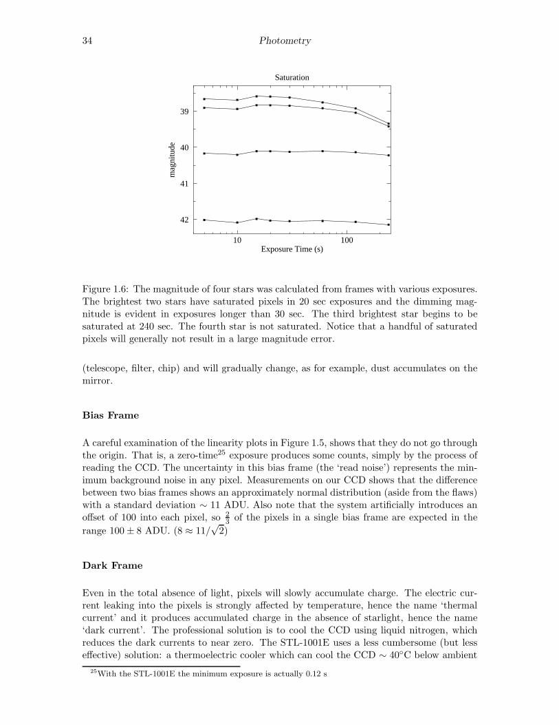
10 100

42

41

40

39

Saturation

Exposure Time (s)

mag

nitu

de

Figure 1.6: The magnitude of four stars was calculated from frames with various exposures.The brightest two stars have saturated pixels in 20 sec exposures and the dimming mag-nitude is evident in exposures longer than 30 sec. The third brightest star begins to besaturated at 240 sec. The fourth star is not saturated. Notice that a handful of saturatedpixels will generally not result in a large magnitude error.

(telescope, filter, chip) and will gradually change, as for example, dust accumulates on themirror.

Bias Frame

A careful examination of the linearity plots in Figure 1.5, shows that they do not go throughthe origin. That is, a zero-time25 exposure produces some counts, simply by the process ofreading the CCD. The uncertainty in this bias frame (the ‘read noise’) represents the min-imum background noise in any pixel. Measurements on our CCD shows that the differencebetween two bias frames shows an approximately normal distribution (aside from the flaws)with a standard deviation ∼ 11 ADU. Also note that the system artificially introduces anoffset of 100 into each pixel, so 2

3of the pixels in a single bias frame are expected in the

range 100 ± 8 ADU. (8 ≈ 11/√

2)

Dark Frame

Even in the total absence of light, pixels will slowly accumulate charge. The electric cur-rent leaking into the pixels is strongly affected by temperature, hence the name ‘thermalcurrent’ and it produces accumulated charge in the absence of starlight, hence the name‘dark current’. The professional solution is to cool the CCD using liquid nitrogen, whichreduces the dark currents to near zero. The STL-1001E uses a less cumbersome (but lesseffective) solution: a thermoelectric cooler which can cool the CCD ∼ 40◦C below ambient

25With the STL-1001E the minimum exposure is actually 0.12 s

Photometry 35

200 400 800 2000 4000

.999

.99

.9

.5

.1

.01

.001

Distribution of Pixel Dark Current

ADU

Perc

entil

e

–20˚ C0˚ C

(a) The distribution of pixel dark current at0◦C and −20◦C. All but a few of the pixelshave a (log)normal distribution of dark cur-rent. About 1% percent of the pixels showmuch larger dark current: these are the ‘hot’pixels. Note that both classes of pixels respondto temperature: lowering the temperature re-duces every pixel’s dark current.

40 45 50 55 60

4000

2000

800

400

200

Along a Row: Dark Current

pixel

AD

U

(b) Part of a row of pixels is displayed at threetemperatures: • = 0◦C, � = −10◦C, H =−20◦C. Isolated hot pixels are randomly sprin-kled throughout the image (here at columns 43and 56). The data here and in (a) are from 15minute dark frames.

0 5 10 15

5000

4000

3000

2000

1000

0

Temperature Reduction ‘cools’ Hot Pixels

Time (min)

AD

U 0˚ C

–10˚ C

–20˚ C

(c) Pixel counts grow with ‘exposure’ time asthe dark current produces ever larger storedcharge in a pixel; of course reducing the tem-perature reduces the dark current.

0 5 10 15

250

200

150

100

Typical Pixels at –20˚ C

Time (min)

AD

U

(d) While it is more evident in this low countdata, there is always random deviation incounts. While we can subtract the average darkcharge, deviations from the average produce‘noise’ in our images. Reducing the temper-ature reduces this noise.

Figure 1.7: Dark frames are ‘exposures’ with the shutter closed. The source of these countsis not starlight, rather a thermally induced current allows charge to accumulate in eachpixel. This ‘dark current’ can be exceptionally large in ‘hot pixels’.

36 Photometry

temperature, reducing the dark currents by more than a factor of 10. The resulting darkcurrents are not negligible for exposures longer than a few minutes. A ‘dark frame’ is sim-ply an ‘exposure’ with the shutter closed; it is a bias frame plus accumulated charge dueto dark currents. A dark frame can be subtracted from an (equally timed) exposed frameto compensate for this non-photon-induced current, however variation in the dark current(‘noise’) results in a corresponding uncertainty in the adjusted pixel counts.

There is tremendous pixel-to-pixel variation in the dark current. About 1% of the pixelshave a dark currents ∼10 times the typical value. The ‘hottest’ pixels26 will saturate in a5 minute exposure at 0◦C. Thus a dark frame looks black except for a handful of bright(‘hot’) pixels; it could be mistaken for the night sky, except the ‘stars’ are not bright disksrather isolated, single hot pixels. Since taking a dark frame takes as much time as a realexposure, use dark frames only when required: when you are taking real data. Simply learnto disregard the sprinkling of isolated hot pixels in non data-taking situations.

Since the dark current depends on temperature, the CCD needs to achieve a stable tem-perature before the dark frames are taken. The CCD has an on-board thermometer, but astable temperature at one point does not mean that the temperature as stabilized through-out the CCD. Direct measures displayed in Figure 1.8 show that it may take several hoursto achieve reproducible dark frames. And the lower the requested temperature the longerit takes to achieve thermal equilibrium. For a requested temperature of −20◦C, 1.8 hoursare required for 95% (e−3 with τ ≈ 0.6 hour) of the excess counts to be eliminated. For arequested temperature of −10◦C, 0.8 hours are required for 95% (e−3 with τ ≈ 0.26 hour)of the excess counts to be eliminated. When requesting particularly low CCD temperaturesit is advisable to take dark frames at the end of the observing session or to cool down thecamera well before sunset. (That is, the obvious time time to take dark frames—at dustbetween taking sky flats and dark-sky frames—may not be the best time to take the darkframes.)

Data Frames

The term ‘object frame’ here refers to a raw CCD frame of the sky as delivered by thecamera-controlling software. If the object frame was not automatically dark-subtracted,there must be a matching (time & temperature) dark frame. A ‘reduced frame’ is an objectframe that has been dark-subtracted and flat-field corrected. By adjusting for non-photon-induced charge and varying pixel sensitivity, we hope our reduced frame shows the actualdistribution of photons. It should be noted that all of these corrections will be applied bymaking the proper requests of the CCD control software. In the end, you should retainboth the fully processed reduced frame and the original object frame.

Basic Plan

Given a reduced frame, determining the number of counts/second from a star is a relativelystraightforward27 task which will be performed (with your help) by the software. This re-

26For example: (265, 742), (68, 97), (233, 866), (266, 166)27Many important details are hereby hidden from view. A short list: (1) determining the background level

to be subtracted from the star pixels (2) determining the proper aperture that encloses all the stars light

Photometry 37

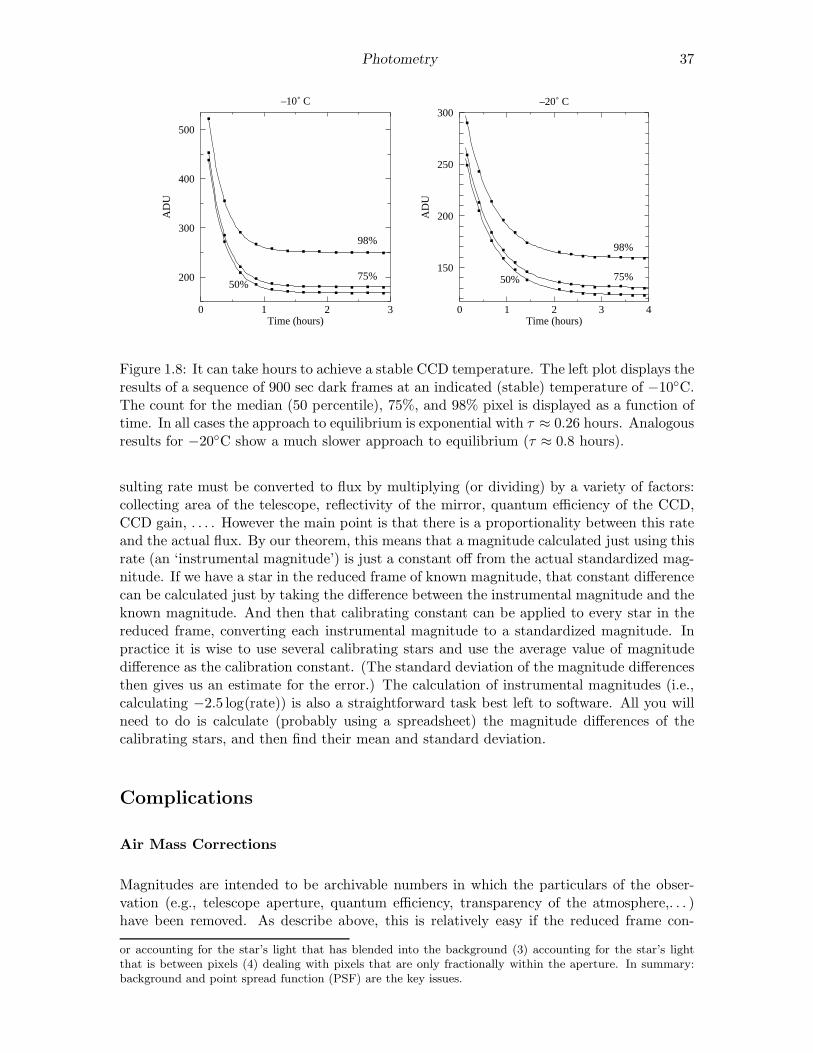
0 1 2 3

500

400

300

200

–10˚ C

Time (hours)

AD

U

50%75%

98%

0 1 2 3 4

300

250

200

150

–20˚ C

Time (hours)

AD

U

50% 75%

98%

Figure 1.8: It can take hours to achieve a stable CCD temperature. The left plot displays theresults of a sequence of 900 sec dark frames at an indicated (stable) temperature of −10◦C.The count for the median (50 percentile), 75%, and 98% pixel is displayed as a function oftime. In all cases the approach to equilibrium is exponential with τ ≈ 0.26 hours. Analogousresults for −20◦C show a much slower approach to equilibrium (τ ≈ 0.8 hours).

sulting rate must be converted to flux by multiplying (or dividing) by a variety of factors:collecting area of the telescope, reflectivity of the mirror, quantum efficiency of the CCD,CCD gain, . . . . However the main point is that there is a proportionality between this rateand the actual flux. By our theorem, this means that a magnitude calculated just using thisrate (an ‘instrumental magnitude’) is just a constant off from the actual standardized mag-nitude. If we have a star in the reduced frame of known magnitude, that constant differencecan be calculated just by taking the difference between the instrumental magnitude and theknown magnitude. And then that calibrating constant can be applied to every star in thereduced frame, converting each instrumental magnitude to a standardized magnitude. Inpractice it is wise to use several calibrating stars and use the average value of magnitudedifference as the calibration constant. (The standard deviation of the magnitude differencesthen gives us an estimate for the error.) The calculation of instrumental magnitudes (i.e.,calculating −2.5 log(rate)) is also a straightforward task best left to software. All you willneed to do is calculate (probably using a spreadsheet) the magnitude differences of thecalibrating stars, and then find their mean and standard deviation.

Complications

Air Mass Corrections

Magnitudes are intended to be archivable numbers in which the particulars of the obser-vation (e.g., telescope aperture, quantum efficiency, transparency of the atmosphere,. . . )have been removed. As describe above, this is relatively easy if the reduced frame con-

or accounting for the star’s light that has blended into the background (3) accounting for the star’s lightthat is between pixels (4) dealing with pixels that are only fractionally within the aperture. In summary:background and point spread function (PSF) are the key issues.

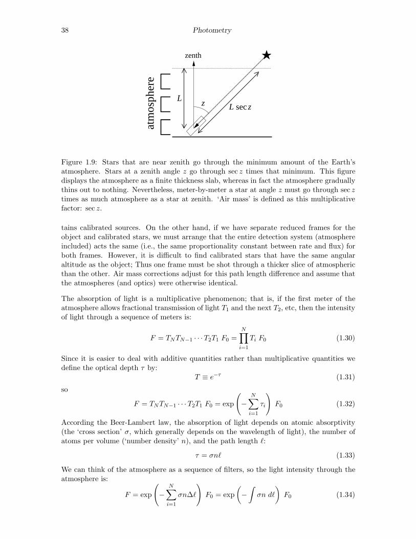
38 Photometry

atm

osph

ere

★zenth

zL

L sec z

Figure 1.9: Stars that are near zenith go through the minimum amount of the Earth’satmosphere. Stars at a zenith angle z go through sec z times that minimum. This figuredisplays the atmosphere as a finite thickness slab, whereas in fact the atmosphere graduallythins out to nothing. Nevertheless, meter-by-meter a star at angle z must go through sec ztimes as much atmosphere as a star at zenith. ‘Air mass’ is defined as this multiplicativefactor: sec z.

tains calibrated sources. On the other hand, if we have separate reduced frames for theobject and calibrated stars, we must arrange that the entire detection system (atmosphereincluded) acts the same (i.e., the same proportionality constant between rate and flux) forboth frames. However, it is difficult to find calibrated stars that have the same angularaltitude as the object; Thus one frame must be shot through a thicker slice of atmosphericthan the other. Air mass corrections adjust for this path length difference and assume thatthe atmospheres (and optics) were otherwise identical.

The absorption of light is a multiplicative phenomenon; that is, if the first meter of theatmosphere allows fractional transmission of light T1 and the next T2, etc, then the intensityof light through a sequence of meters is:

F = TNTN−1 · · ·T2T1 F0 =N∏

i=1

Ti F0 (1.30)

Since it is easier to deal with additive quantities rather than multiplicative quantities wedefine the optical depth τ by:

T ≡ e−τ (1.31)

so

F = TNTN−1 · · ·T2T1 F0 = exp

(

−N∑

i=1

τi

)

F0 (1.32)

According the Beer-Lambert law, the absorption of light depends on atomic absorptivity(the ‘cross section’ σ, which generally depends on the wavelength of light), the number ofatoms per volume (‘number density’ n), and the path length ℓ:

τ = σnℓ (1.33)

We can think of the atmosphere as a sequence of filters, so the light intensity through theatmosphere is:

F = exp

(

−N∑

i=1

σn∆ℓ

)

F0 = exp

(

−∫

σn dℓ

)

F0 (1.34)

Photometry 39

1.8 2.0 2.2 2.4 2.6 2.8

31.20

31.15

31.10

31.05

31.00

Air Mass

v–V

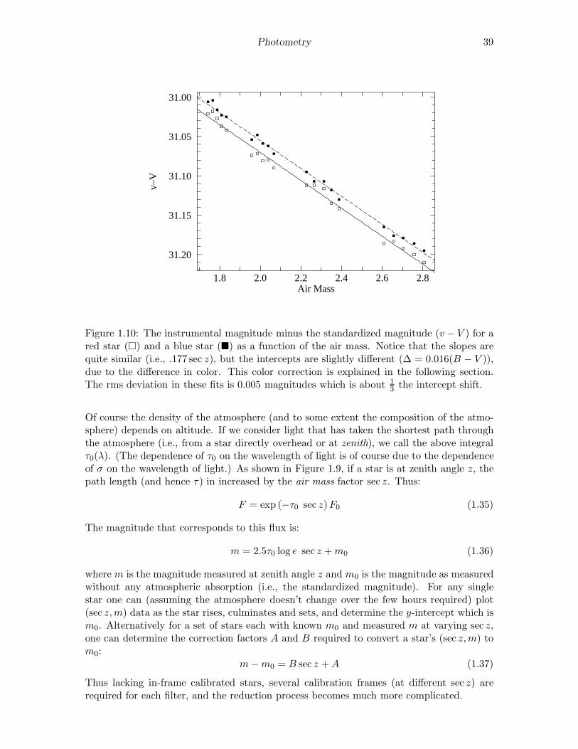
Figure 1.10: The instrumental magnitude minus the standardized magnitude (v − V ) for ared star (�) and a blue star (�) as a function of the air mass. Notice that the slopes arequite similar (i.e., .177 sec z), but the intercepts are slightly different (∆ = 0.016(B − V )),due to the difference in color. This color correction is explained in the following section.The rms deviation in these fits is 0.005 magnitudes which is about 1

3the intercept shift.

Of course the density of the atmosphere (and to some extent the composition of the atmo-sphere) depends on altitude. If we consider light that has taken the shortest path throughthe atmosphere (i.e., from a star directly overhead or at zenith), we call the above integralτ0(λ). (The dependence of τ0 on the wavelength of light is of course due to the dependenceof σ on the wavelength of light.) As shown in Figure 1.9, if a star is at zenith angle z, thepath length (and hence τ) in increased by the air mass factor sec z. Thus:

F = exp (−τ0 sec z)F0 (1.35)

The magnitude that corresponds to this flux is:

m = 2.5τ0 log e sec z + m0 (1.36)

where m is the magnitude measured at zenith angle z and m0 is the magnitude as measuredwithout any atmospheric absorption (i.e., the standardized magnitude). For any singlestar one can (assuming the atmosphere doesn’t change over the few hours required) plot(sec z,m) data as the star rises, culminates and sets, and determine the y-intercept which ism0. Alternatively for a set of stars each with known m0 and measured m at varying sec z,one can determine the correction factors A and B required to convert a star’s (sec z,m) tom0:

m − m0 = B sec z + A (1.37)

Thus lacking in-frame calibrated stars, several calibration frames (at different sec z) arerequired for each filter, and the reduction process becomes much more complicated.

40 Photometry

–8 –6 –4 –2 0 2 4 6 8

60

40

20

0

–20

Air Mass

Hour Angle

Dec

linat

ion

1.1 1.2 1.5 2.0 2.5

3.0

Z

Figure 1.11: Air mass (sec z) depends on where a star is in the sky. Air mass is plotted hereas a function of the star’s declination and hour angle for the SJU observatory location. Zmarks zenith, where the minimum (1) air mass is found.

Note that the zenith angle z can be calculated28 from:

cos z = sin δ sin ϕ + cos δ cos h cos ϕ (1.38)

where δ and h are the star’s declination and hour angle and ϕ is the observatory’s latitude.The above terms from astrometry (declination, hour angle, altitude, zenith, right ascension,. . . ) are part of the everyday vocabulary of astronomers. If you are not familiar with theseterms you should read the following online tutorials:

• http://www.physics.csbsju.edu/astro/CS/CSintro.html

• http://www.physics.csbsju.edu/astro/sky/sky.01.html

• http://www.physics.csbsju.edu/astro/terms.html

For example at SJU (ϕ = 45◦34.5′) for stars on the celestial equator (δ = 0), the minimumair mass (at h = 0h) is sec z = 1.43. The sequence of air masses: sec z=1.5, 2.0, 2.5, 3.0occurs at hour angles h = ±1.18h,±2.96h,±3.68h,±4.10h. Figure 1.11 plots these air massvalues for other declinations.

Color Corrections

We learned in the above section that the Earth’s atmosphere acts as a non-negligible filter,attenuating (absorbing or scattering, generally reducing) starlight before it reaches our

28xephem can do this calculation for you

Photometry 41

Fλ Fλ

λλ

hot star cool star

B B7777777777777777777777777777777777777777777777777777777777777777

7777777777777777777777777777777777777777777777777777777777777777777777777777777777777777777777777777777777777777

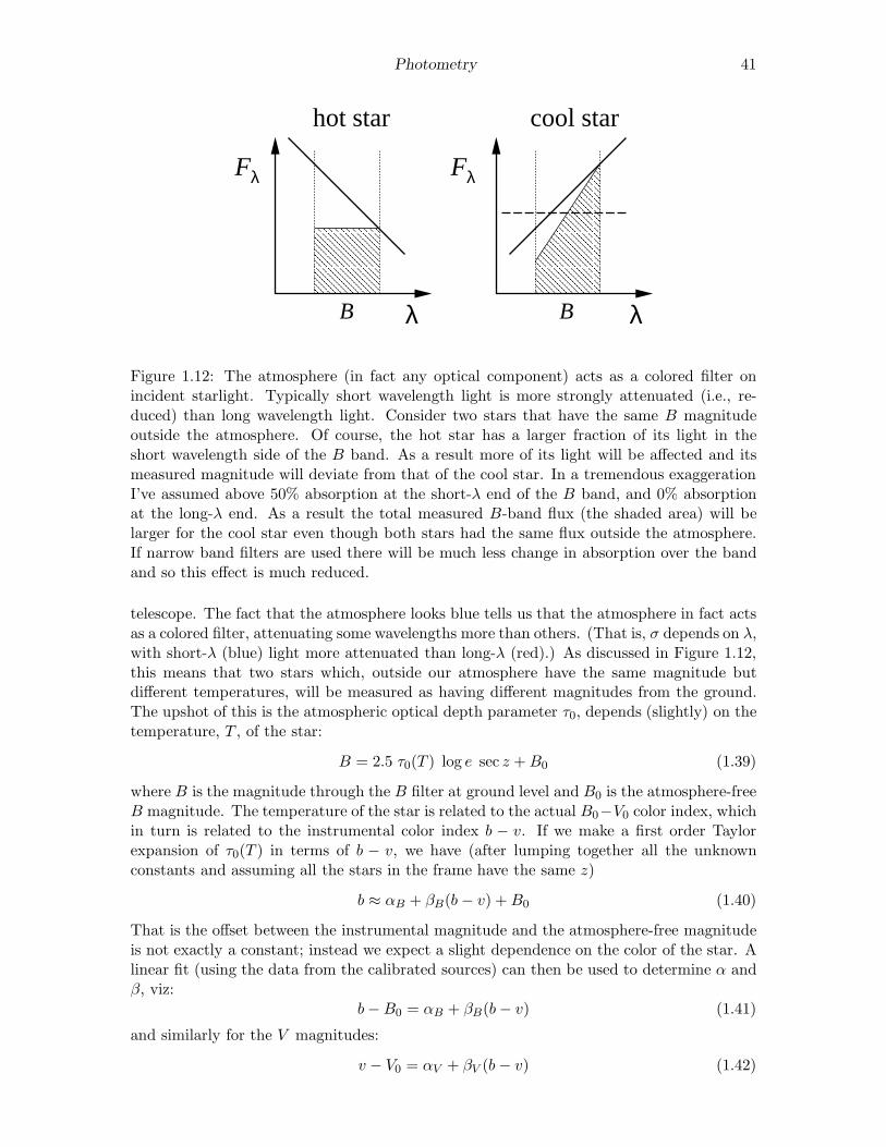
Figure 1.12: The atmosphere (in fact any optical component) acts as a colored filter onincident starlight. Typically short wavelength light is more strongly attenuated (i.e., re-duced) than long wavelength light. Consider two stars that have the same B magnitudeoutside the atmosphere. Of course, the hot star has a larger fraction of its light in theshort wavelength side of the B band. As a result more of its light will be affected and itsmeasured magnitude will deviate from that of the cool star. In a tremendous exaggerationI’ve assumed above 50% absorption at the short-λ end of the B band, and 0% absorptionat the long-λ end. As a result the total measured B-band flux (the shaded area) will belarger for the cool star even though both stars had the same flux outside the atmosphere.If narrow band filters are used there will be much less change in absorption over the bandand so this effect is much reduced.

telescope. The fact that the atmosphere looks blue tells us that the atmosphere in fact actsas a colored filter, attenuating some wavelengths more than others. (That is, σ depends on λ,with short-λ (blue) light more attenuated than long-λ (red).) As discussed in Figure 1.12,this means that two stars which, outside our atmosphere have the same magnitude butdifferent temperatures, will be measured as having different magnitudes from the ground.The upshot of this is the atmospheric optical depth parameter τ0, depends (slightly) on thetemperature, T , of the star:

B = 2.5 τ0(T ) log e sec z + B0 (1.39)

where B is the magnitude through the B filter at ground level and B0 is the atmosphere-freeB magnitude. The temperature of the star is related to the actual B0−V0 color index, whichin turn is related to the instrumental color index b − v. If we make a first order Taylorexpansion of τ0(T ) in terms of b − v, we have (after lumping together all the unknownconstants and assuming all the stars in the frame have the same z)

b ≈ αB + βB(b − v) + B0 (1.40)

That is the offset between the instrumental magnitude and the atmosphere-free magnitudeis not exactly a constant; instead we expect a slight dependence on the color of the star. Alinear fit (using the data from the calibrated sources) can then be used to determine α andβ, viz:

b − B0 = αB + βB(b − v) (1.41)

and similarly for the V magnitudes:

v − V0 = αV + βV (b − v) (1.42)

42 Photometry

FWHM

FWHM

bright stardim star

pixel

AD

U

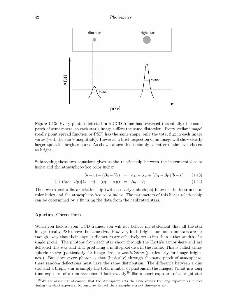
Figure 1.13: Every photon detected in a CCD frame has traversed (essentially) the samepatch of atmosphere, so each star’s image suffers the same distortion. Every stellar ‘image’(really point spread function or PSF) has the same shape, only the total flux in each imagevaries (with the star’s magnitude). However, a brief inspection of an image will show clearlylarger spots for brighter stars. As shown above this is simply a matter of the level chosenas bright.

Subtracting these two equations gives us the relationship between the instrumental colorindex and the atmosphere-free color index:

(b − v) − (B0 − V0) = αB − αV + (βB − βV )(b − v) (1.43)

[1 + (βV − βB)] (b − v) + (αV − αB) = B0 − V0 (1.44)

Thus we expect a linear relationship (with a nearly unit slope) between the instrumentalcolor index and the atmosphere-free color index. The parameters of this linear relationshipcan be determined by a fit using the data from the calibrated stars.

Aperture Corrections

When you look at your CCD frames, you will not believe my statement that all the starimages (really PSF) have the same size. However, both bright stars and dim stars are farenough away that their angular diameters are effectively zero (less than a thousandth of asingle pixel). The photons from each star shoot through the Earth’s atmosphere and aredeflected this way and that producing a multi-pixel disk in the frame. This is called atmo-spheric seeing (particularly for image size) or scintillation (particularly for image bright-ness). But since every photon is shot (basically) through the same patch of atmosphere,these random deflections must have the same distribution. The difference between a dimstar and a bright star is simply the total number of photons in the images. (That is a longtime exposure of a dim star should look exactly29 like a short exposure of a bright star

29We are assuming, of course, that the atmosphere acts the same during the long exposure as it doesduring the short exposure. No surprise: in fact the atmosphere is not time-invariant.

Photometry 43

if the two cases produce the same number of photons.) To see that the distributions areidentical you should look at the full width at half maximum (FWHM) of the PSF: Firstdetermine the peak count in an image, and then find the circle at which the count is halfof this maximum. The diameter of the circle (typically a few arcsec) is the FWHM.

Because of the obvious difference in the image size, when totaling the counts in a stellarimage one is tempted to expand or reduce the range of pixels included as part of a starto match the apparent size of that star. Doing this means that an accurate count willbe obtained for bright stars, whereas counts will be excluded in dim stars. While thisdoesn’t sound like a particularly horrendous idea, recall that our theorem states that if wecapture a consistent fraction of the counts in every star, all our instrumental magnitudeswill just be a constant off from the standardized magnitudes. So a consistent fraction of thecounts may be combined with all the other proportionality constants in the final differencebetween instrumental magnitude and standardized magnitude. Now there may be occasionswhere we must adjust the aperture used for magnitude calculation (for example to exclude aneighboring star), however then inconsistencies (and hence errors) are then being generated.The disadvantage of using a constant aperture is relatively more noise-prone ‘background’pixels will be included in dim stars. There are a variety of solutions to this problems(generally under the heading of PSF fitting), however they are beyond the aims of this lab.

The blurring of star images (i.e., PSF) depends both on atmospheric seeing and the ad-justment of the telescope. Clearly an out-of-focus telescope (see below) will produce largerstar images than a properly focused telescope. It should also be noted that the telescope’s‘optical aberrations’ result in additional blurring near the edge of the telescope’s field ofview.

Focus

The aim of focus is to achieve that smallest possible FWHM, so each star’s light is con-centrated in the fewest possible number of pixels. Since every pixel comes with a certainbackground ‘noise’, fewer pixels means less noise in the stellar magnitude. You should planon spending a good bit of time (maybe a half hour) trying to achieve the best possible focus.There are two approaches to monitoring improved focus: (1) monitor the peak count in abright star (∼ 4 mag), (2) watch for the appearance of numerous dim stars as their peakgets above the ‘bright’ level. (You must learn to ignore the apparent size of bright stars:it is a poor measure of good focus.) A complicating factor is that both (1) and (2) varyindependently of focus adjustments since atmospheric seeing varies from second to second,and since photon counts should be expected to vary ∼

√N .

Software

xephem

xephem is planetarium software designed to display various types of night-sky maps inadvance of observing. You will also use it to tabulate astrometry data relevant to yourobservations. The file using.xephem.txt describes how to use this program to produce thetables and maps required for the pre-observation phase of the lab. In addition you can use

44 Photometry

it for astrometry and photometry on .fit images (although I recommend gaia below forthese reductions).

Aladin

Aladin is a front-end to various astronomy databases on the internet. You will use it tofind images to use as finder maps and to identify (and obtain data on ) the stars in thoseimages. The Aladin server and SkyView+ are often a good sources of images; Simbad isthe usual source for stellar information. Sometimes just information from the SAO catalogis required; then VizieR can be used to access just the SAO catalog. You will use Aladin

mostly in the pre-observation phase. The file using.Aladin.txt briefly describes how touse this program to produce the maps and data required for the pre-observation phase ofthe lab. Note: NASA has a very handy web page30 that also allows you to do many of thesethings. gaia (see below) is also and excellent way to make finder maps.

CCDops

CCDOps is software used to control the camera and create/save CCD frames. You will beusing a small fraction of its capabilities. Typical commands will be: to set the tempera-ture (cooling) of the CCD, focus, grab images (set the exposure time and perhaps take adark frame), examine images (histogram, crosshair), save images (in both .SBIG and .fit

formats), and reduce images by dark-subtracting, flat-fielding or averaging.

ccdview

ccdview will be used as a first-look program. Immediately following your observing nightyou will want to examine the image files (stored on /media/disk). (At the same time youshould put copies of the important frames in your linux directory.) While you can usethis program to determine magnitudes, gaia (see following) will do a better job. The fileusing.ccdview.txt briefly describes how to use this program.

gaia

gaia is the recommended reduced-frame analysis program. In order to use gaia you willneed to convert your .SBIG frame into a ndf frame (.sdf) using the program sbig2ndf.The file using.gaia.txt briefly describes how to use this program.

IRAF

IRAF is the Image Reduction and Analysis Facility, a general purpose software systemfor the reduction and analysis of astronomical data. It is the standard for professionalastronomers: designed for the expert user—with no compromises for the beginner. While

30http://skyview.gsfc.nasa.gov/: start with 1000×1000 pixel Digitized Sky Survey image with 0.5◦

Image Size, B-W Log Inverse Color Table, and a Grid

Photometry 45

its use is encouraged for those thinking of becoming astronomers, I cannot recommend itfor this lab.

Planning to Observe

Minnesota weather is is unpredictable31 and we need an extraordinary, no-visible-cloudsnight. We must be prepared to use any/every of these rare nights on short notice. Ofcourse, you have other commitments (your concert, the night before your math/physicsexam, the St. Thomas game. . . ), the aim here is to communicate those constraints to meand to your lab partners in well in advance. Thus you will need to carefully record yourschedule a lunar month ahead. Note that Murphy’s Law guarantees that if you forget toX-out some important night (your girlfriend’s birthday, the day before your term paper isdue, a ‘free’ day), that night will be clear, and somebody (I hope not me!) is going tobe disappointed. My family commitments and intro astro labs are going X-out all Sundaynights and many Monday and Wednesday nights.

Before each full moon, mark on the class calendar the dates you and your lab partner(s)are committed to observe.

Since clear nights are precious, ‘go’ days need a well-thought-out plan. If you’re followingthe standard project, your plan involves a target whose frame will include several starswith known32 B,V,R, I magnitudes. Thus you need to: (A) Find a target that has therequired stars. (Stars with recorded R magnitudes are relatively rare.) (B) Know wherethose standard stars are in your target (so you can aim so your CCD frames to include thestars you need). (C) Know where your target is among the neighboring stars (so if yourfirst try at finding the target fails, you have a plan [not ‘hunt-and-peck’] for getting to theright spot). (D) And of course, know that your target is well above the horizon when youare planning to observe. While the standard project does not require additional standardstars, you may want you to record alternative (out-of-frame) standards.

Thus, you must produce (and turn in) the pre-observation documents described below. Us-ing the following new moon as a date, use xephem, to select your targets. The problem is tofind a star cluster that has the required calibrated stars. For example, in early Septemberxephem makes M39 or NGC 6871 obvious choices. However, I’m unable to find any calibrat-ing R magnitudes in those clusters. (Of course, correcting for air mass and using calibratedsources outside of the cluster is an option.) Starting with the options listed in Table 1.2,clusters between NGC 6940 (air mass 1.2) and M5 (air mass 2.0) are OK; NGC 6940 orNGC 6738 seems to have the smallest air mass. http://obswww.unige.ch/webda/ showslots of R and I magnitude stars well within the capabilities of our system (V < 13), soeither looks like a fine choice.

31http://www.physics.csbsju.edu/astro/ has a link designed to report (guess) sky conditions at theSJU observatory. It cannot be relied on, but I believe it’s the best available information. Note: black isgood for this clear sky clock.

32Professionally, only very carefully measured ‘standard’ stars—for example those measured by Landoltor Stetson—would be used for calibration. For the purposes of this lab you may use any star that has a‘book’ magnitude. It is not at all unusual for such literature magnitudes to have 10% errors

46 Photometry

Pre-observation Checklist

The following should be prepared before each full moon (4-Sep-09, 4-Oct-09, 2-Nov-09):

1. Sign up for ‘go’ days during the following lunar month.

2. Using xephem set for the date of the following new moon print out the following:

(a) A Sky View showing the entire sky with the labeled location of the target.It is helpful to label the brightest stars with the Meade * number from theMeade250.edb file.

(b) A .xephem/datatbl.txt file recording basic data (RA, dec, air mass, . . . ) forthe target for several times through the night.

(c) A copy&pasted list of basic data on the SAO stars used to locate the target andselected standard stars (‘LX200 stars’)—perhaps copy&pasted into the abovefile. Find and record nearby mag ∼4 stars to help achieve sharp focus. The fileusing.xephem.txt describes what data you need to have recorded.

3. Using Aladin (or web-based skyview.gsfc.nasa.gov) print out the following findingcharts for your target cluster:

(a) a low magnification (degree scale) image showing the relationship between theLX200 star and the desired CCD frame.

(b) an image scaled to about 2× the CCD frame showing exactly the desired CCDframe. (Since the target CCD frame must include calibrated stars, clearly youmust know where the calibrated stars are in the target.) Record the RA and decfor your target frame(s).

Learning to effectively use these pre-observation programs will be a bit of a challenge andtake several hours, so do not procrastinate and feel free to seek my help. In addition to theusual problems of learning new software, you will need to learn how to make the web-basedastronomy databases find the information you need.

Example 1: Plan for Lunar Month starting 21-July-2005

Immediately on starting xephem, Set the location: SJU Observatory, click on the Calendar

for the following new moon (“NM”, in this case 4-August-2005) and enter a Local Time of21:00 (9 p.m.). Hit Update so xephem is ready to display the sky at that time. View→Sky

View then displays the night sky for that location/date/time. (Print a copy of this sky viewas described in using.xephem.txt and record: UTC Time: 2:00, Sidereal: 16:37.) IC 4665is the obvious target; its RA (listed in Table 1.2) is most nearly equal to the sidereal timeand hence it is near the meridian, However, with a diameter of 70′, IC 4665 is much largerthan the CCD frame, so only a small fraction of it will be imaged—a fraction that mustinclude several calibrated stars. A visit to the IC 4665 cluster web page33 finds a couple ofdozen of VRIc observations. I copy and paste that data into a spreadsheet, and then seekcorresponding UBV CCD data. The result is 12 stars with the full set of BV RI data. Next

33http://obswww.unige.ch/webda/

Photometry 47

we need to find a CCD frame that will include as many of these stars as possible. (It is ofcourse possible to use a different set of stars to calibrate different filters, but it will be easierif one set of stars will serve for all calibrations.) Surprisingly, most of the 12 stars haveSAO34 identifications; only three stars must be located by RA and dec. Aladin can find alow magnification (1.5◦ × 1.5◦) image of IC 4665. (Print this image as a low magnificationfinder chart.) A request to VizieR for the SAO catalog objects near IC 4665 allows meto locate the calibrated sources found above. Since IC 4665 is much larger than our CCDframe, we aim for the largest possible subset of these stars. A CCD frame centered nearSAO 122742 will pick up four fully calibrated stars (73, 82, 83, 89). Simbad gives B−V datafor several other bright stars in this frame (e.g., TYC 424-75-1, Cl* IC4665 P44), but I don’tfind additional R−I data in Simbad. Returning to obswww.unige.ch, I find (depending onthe exact position of the CCD frame) it may be possible to include R − I calibrated stars67, 76, 84, & 90. You should decide exactly how to place the CCD frame and locate thecalibrated stars on a finder chart that is about 2× the size of the CCD frame. For focusstars consider SAO 122671 (mag=3) and SAO 123005 (mag=5). Note that SAO 122723would make a good (bright: mag=6.8) star to aim the LX200 near this object. (I callsuch aiming/finding stars ‘LX200 stars’. The LX200 object library includes all SAO starsbrighter than magnitude 7, but any bright star can help assure the telescope is aimed atwhat you intend (and that the telescope’s reported RA/dec are accurate). You can load theSAO LX200.edb database into xephem to display the LX200 stars; SAO mag75.edb includesabout twice as many stars (down to magnitude 7.5); SAO full.edb includes about a quarterof a million stars (down below magnitude 9).

In such a large cluster, it would be wise to select additional fields, for example one centerednear SAO 122709. A CCD frame there might include R− I calibrated stars: 39, 40, 43, 44,49, 50, 58, 62.

To select alternative standards. . . WIYN has a web page35 with recommended standard starregions. (WIYN’s stars are designed for a large telescope, and hence would require longexposures on our telescope). Peter Stetson’s extensive list of standards is also online36.The xephem databases LONEOS.edb, Landolt83.edb and Buil91.edb contain shorter listsof brighter stars: < 13mag, ∼9.5mag and < 8mag respectively.) Generally these goodstandard stars will be well-separated from the target, so air mass air mass correction wouldbe required. (Since I have internal ‘calibrated’ sources, I’m not required to take CCD framesof these standards, however I’ve decided to ‘be prepared’ and hence have recorded the basicdata I would need to observe them.) I select: #109 (PG1633+099, at RA=16:35, LX200star: SAO 121671), #121 (110 506, at RA=18:43, LX200 star: SAO 142582), and #125(111 1969, at RA=19:37, LX200 star: SAO 143678, also see: SAO 124878). These standardstars can be marked as xephem Favorites from the UBVRI.edb database. These sourcesshould span a good range of air mass in the general direction of the target. Following theinstructions in using.xephem.txt, I create a file of basic location data for my target andstandard fields. By default, this file is: .xephem/datatbl.txt and can be printed (% lp

filename) or edited (% kwrite filename).

34Smithsonian Astrophysical Observatory—a standard catalog of ‘bright’ stars.35http://www.noao.edu/wiyn/obsprog/images/tableB.html36http://cadcwww.hia.nrc.ca/standards/

48 Photometry

Example 2: Plan for Lunar Month starting 19-August-2005

After Setting xephem for location: SJU Observatory, the new moon date 3-September-2005, and Local Time 21:00 (9 p.m.), I find and record: UTC Time: 2:00, Sidereal: 18:35.NGC 6633, whose RA is most nearly equal to the sidereal time and hence is near themeridian, is the obvious target. After adding NGC 6633 to xephem Favorites and loading theSAO database (Data→Files; Files→SAO mag75.edb), it’s easy to zoom in (lhs scroll bar) onNGC 6633 and find the nearby bright (5.7 mag) star SAO 12351637 , which would be a goodstar to steer the LX200. For focus stars consider SAO 122671 (mag=3) and SAO 123377(mag=5). A visit to the NGC 6633 cluster web page38 finds six VRIe observations for R.Cross-reference shows that all six are ∼ 8 mag SAO stars39, however only two (50 & 70) arein the central region of the cluster. (They could also be found using SAO full.edb.) Stetsonreports BV I data for NGC 6633, however the brightest ten of his stars are ∼ 13 mag,which is 100× dimmer than the ∼ 8 mag R-mag stars. Thus different frames are requiredto properly expose the Stetson standards and the R ‘standards’.

Using the Buil91.edb database, I can find bright standard stars: SAO 085402, SAO 141956,SAO 145050. These bright SAO stars are themselves LX200 stars.

Example 3: Plan for Lunar Month starting 21-June-2005

After Setting xephem for location: SJU Observatory, the new moon date 6-July-2005, andLocal Time 22:00 (10 p.m. — it’s not dark at 9 p.m.), I find and record: UTC Time: 3:00,Sidereal: 15:43. Because of its larger declination, Upgren 1 has a bit less air mass thanNGC 6633, so it becomes the target. Upgren 1 is not in xephem’s databases, so it must beadded to Favorites following the procedure recorded in using.xephem.txt. A visit to theUpgren 1 cluster web page40 finds seven stars with VRIc and UBV observations. Howeverthe color index disagreements are of order 0.05, so we can use this as an opportunity to findthe correct values. Using the Landolt83.edb database, I find three neighboring standardstars with a range of colors: HD 102056 (LX200 star: SAO 81968, bluer than the Upgren1 stars), HD 106542 (LX200 star: SAO 100009, redder than the Upgren 1 stars), andHD 107146 (LX200 star: SAO 100038, similar to the Upgren 1 stars). Using the Oja96.edbdatabase, I find two very close stars with similar colors: BD+35 2356 and BD+34 2338.(For these dimmer, ∼10 magnitude, stars finder charts are required.) ∗#133 (SAO 63257,with mag 5 partner 63256) is a neighboring mag 3 star, SAO 44230 is a mag 4 star — bothcan help focus and alignment. SAO 63118 is the nearest LX200 star to Upgren 1 (sinceUpgren 1 is not in the LX200 catalog of clusters, the final jump must be made based onRA/dec). All but one of the Upgren 1 seven stars is an SAO star; they are all easy toidentify with Aladin. (FYI: spiral galaxies M94 and M63 might be worth a look.)

Target and standards were fairly close together and near the meridian during the measure-ments, with airmass varying from 1.01 to 1.14. This was not a sufficient range to detectairmass correction terms. Increasing airmass dims and reddens stars. As a result calibratedstars viewed through a larger air mass will have a smaller constant in the color calibration

37VizieR reports R = 5.703, for this star, which may serve as an additional standard. FYI: this star isalso known as: HD 170200 and HR 6928.

38Again: http://obswww.unige.ch/webda/39These dim SAO stars are not in SAO mag75.edb so I located them using Aladin40Again: http://obswww.unige.ch/webda/

Photometry 49

Names Constellation Right Ascension Declination Diameter Reddening(2000) (2000) (arcmin) (mag)

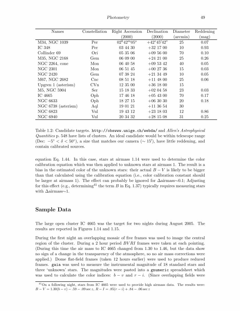
M34, NGC 1039 Per 02h42m05s +42◦45′42” 25 0.07IC 348 Per 03 44 30 +32 17 00 10 0.93Collinder 69 Ori 05 35 06 +09 56 00 70 0.10M35, NGC 2168 Gem 06 09 00 +24 21 00 25 0.26NGC 2264, cone Mon 06 40 58 +09 53 42 40 0.05NGC 2301 Mon 06 51 45 +00 27 36 15 0.03NGC 2420 Gem 07 38 24 +21 34 49 10 0.05M67, NGC 2682 Cnc 08 51 18 +11 48 00 25 0.06Upgren 1 (asterism) CVn 12 35 00 +36 18 00 15M5, NGC 5904 Ser 15 18 33 +02 04 58 23 0.03IC 4665 Oph 17 46 18 +05 43 00 70 0.17NGC 6633 Oph 18 27 15 +06 30 30 20 0.18NGC 6738 (asterism) Aql 19 01 21 +11 36 54 30NGC 6823 Vul 19 43 12 +23 18 03 12 0.86NGC 6940 Vul 20 34 32 +28 15 08 31 0.25

Table 1.2: Candidate targets. http://obswww.unige.ch/webda/ and Allen’s Astrophysical

Quantities p. 548 have lists of clusters. An ideal candidate would be within telescope range(Dec: −5◦ < δ < 50◦), a size that matches our camera (∼ 15′), have little reddening, andcontain calibrated sources.

equation Eq. 1.44. In this case, stars at airmass 1.14 were used to determine the colorcalibration equation which was then applied to unknown stars at airmass 1. The result is abias in the estimated color of the unknown stars: their actual B − V is likely to be biggerthan that calculated using the calibration equation (i.e., color calibration constant shouldbe larger at airmass 1). The effect can probably be ignored for ∆airmass∼0.1; Adjustingfor this effect (e.g., determining41 the term B in Eq. 1.37) typically requires measuring starswith ∆airmass∼1.

Sample Data

The large open cluster IC 4665 was the target for two nights during August 2005. Theresults are reported in Figures 1.14 and 1.15.

During the first night an overlapping mosaic of five frames was used to image the centralregion of the cluster. During a 2 hour period BV RI frames were taken at each pointing.(During this time the air mass to IC 4665 changed from 1.30 to 1.46, but the data showno sign of a change in the transparency of the atmosphere, so no air mass corrections wereapplied.) Dome flat-field frames (taken 12 hours earlier) were used to produce reducedframes. gaia was used to measure the instrumental magnitude of 18 standard stars andthree ‘unknown’ stars. The magnitudes were pasted into a gnumeric spreadsheet whichwas used to calculate the color indices: b − v and r − i. (Since overlapping fields were

41On a following night, stars from IC 4665 were used to provide high airmass data. The results were:B − V = 1.30(b − v) − .59 − .09 sec z, R − I = .85(r − i) + .84 − .06 sec z

50 Photometry

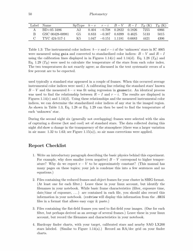
Label Name SpType b − v r − i B − V R − I TB (K) TR (K)

A BD+05 3486 A2 0.404 −0.708 0.2822 0.1826 7255 6966B GSC 00428-00981 G5 0.833 −0.387 0.8399 0.4625 5133 5015C TYC 424-517-1 K5 1.047 −0.151 1.1181 0.6683 4421 4306

Table 1.3: The instrumental color indices: b− v and r− i of the ‘unknown’ stars in IC 4665were measured using gaia and converted to standardized color indices: B − V and R − Iusing the calibration lines displayed in in Figures 1.14(c) and 1.14(d). Eq. 1.28 (TB) andEq. 1.29 (TR) were used to calculate the temperature of the stars from each color index.The two temperatures do not exactly agree; as discussed in the text systematic errors of afew percent are to be expected.

used typically a standard star appeared in a couple of frames. When this occurred averageinstrumental color indices were used.) A calibrating line relating the standard stars’ knownB − V and the measured b − v was fit using regression in gnumeric. An identical processwas used to find the relationship between R − I and r − i. The results are displayed inFigures 1.14(c) and 1.14(d). Using these relationships and the measured instrumental colorindices, we can determine the standardized color indices of any star in the imaged region.As shown in Table 1.3, Eq. 1.28 or Eq. 1.29 can then be used to find the temperature ofeach ‘unknown’ star.

During the second night six (generally not overlapping) frames were selected with the aimof capturing a diverse (hot and cool) set of standard stars. The data collected during thisnight did show a change in the transparency of the atmosphere (there was a larger variationin air mass: 1.32 to 1.63; see Figure 1.15(a)), so air mass corrections were applied.

Report Checklist

1. Write an introductory paragraph describing the basic physics behind this experiment.For example, why does smaller (even negative) B − V correspond to higher temper-ature? Why do we expect v − V to be approximately constant? (This manual hasmany pages on these topics; your job is condense this into a few sentences and noequations.)

2. Files containing the reduced frames and object frames for your cluster in SBIG format.(At least one for each filter.) Leave these in your linux account, but identify thefilenames in your notebook. While basic frame characteristics (filter, exposure time,date/time of exposure, . . . ) are contained in each file, you should also record thisinformation in your notebook. (ccdview will display this information from the .SBIG

files in a format that allows easy copy & paste.)

3. Files containing the flat-field frames you used to flat-field your images. (One for eachfilter, but perhaps derived as an average of several frames.) Leave these in your linuxaccount, but record the filenames and characteristics in your notebook.

4. Hardcopy finder charts, with your target, calibrated stars and nearby SAO LX200stars labeled. (Similar to Figure 1.14(a).) Record an RA/dec grid on your findercharts.

Photometry 51

(a) This Digitized Sky Survey image shows thecentral ∼ 50′

× 25′ region of the open clusterIC 4665. The standard stars of J.W. Menziesand F. Marang (MNRAS, 282, 313–316 (1996))are labeled along with three ‘unknown’ stars:A, B, C.

.2 .4 .6 .8 1.0 1.2 1.4 1.6

28.26

28.24

28.22

28.20

28.18

28.16

28.14

v–V Calibration

b–v

v–V

(b) There is little evidence for a significantcolor correction in this data set. See Eq. 1.42.

.2 .4 .6 .8 1.0 1.2 1.4 1.6

1.5

1.0

.5

0

B–V Calibration

b–v

B–V

(c) Calibration of the standardize color indexB −V in terms of the instrumental color indexb − v. See Eq. 1.44.

–1.0 –.8 –.6 –.4 –.2 0 .2

1.0

.8

.6

.4

.2

0

R–I Calibration

r–i

R–I

(d) Calibration of the standardize color indexR − I in terms of the instrumental color indexr − i.

Figure 1.14: An overlapping mosaic of five frames was used to image the central region of theopen cluster IC 4665. This region includes 18 standard stars which were used to calibratethe relationships between standardized color indices and instrumental color indices. Usingthese relationships and the measured instrumental color indices, we can determine thestandardized color indices of any star in the imaged region.

52 Photometry

1.35 1.40 1.45 1.50 1.55 1.60

31.46

31.44

31.42

31.40

31.38

31.36

Air Mass Corrections

Air Mass

<b–

B>

or

<i–

I>

(a) Short wavelengths are more affected byatmospheric absorption than long; the aboveshows the effect on B magnitudes (filledsquares) and I magnitudes (open circles). They axis displays the difference between instru-mental and standardized magnitudes averagedover all the blue stars in the frame.

.6 .8 1.0 1.2 1.4 1.6 1.8

30.96

30.94

30.92

30.90

30.88

30.86

Color Correction

b–v

v–V

(b) Color correction is evident in this data set,but both air mass and color correction shouldbe applied to this data. This full result was:v − V = 30.611 + 0.179 sec z + 0.048(b − v).The rms variation from this line was less than0.02 mag.

.6 .8 1.0 1.2 1.4 1.6 1.8

1.5

1.0

.5

0

B–V Color Calibration

b–v

B–V

(c) Calibration of the standardize color indexB −V in terms of the instrumental color indexb − v.B − V = −0.67 + 1.29(b − v)

–.8 –.6 –.4 –.2 0 .2

.8

.6

.4

.2

0

R–I Color Calibration

r–i

R–I

(d) Calibration of the standardize color indexR − I in terms of the instrumental color indexr − i.R − I = 0.80 + 0.86(r − i)

Figure 1.15: Six frames were used to image 22 standard stars in the open cluster IC 4665.The selected stars have a wide variation in color in order to to achieve robust color cali-brations. During the 2+ hours of data collection the air mass increased from 1.32 to 1.63and the resulting increase in atmospheric absorption increased (dimmed) B,V,R, and Imagnitudes in proportion to the air mass (see Figure 1.15(a)).

Photometry 53

5. xephem datafile containing basic data (RA, Dec, altitude, air mass for each observationnight). Print this out and tape in your lab notebook.

6. Table containing the basic data on your calibrated stars, including standard namesand magnitudes. (Perhaps included in the below file.)

7. Spreadsheet file, reasonably well documented, containing known and instrumentalmagnitudes. For each filter, calculate instrumental−standard magnitudes (e.g., v−V )and record the basic statistics (mean, standard deviation). (Note that aside from asmall color correction, we expect v − V to be constant.) You should use this spread-sheet to calculate instrumental color indices and prepare the data for the followingplots. Self document these calculations before you print out the data table for inclu-sion in your notebook.

8. Hardcopy plot of B − V vs. instrumental b − v with a fitted line. (Similar to Fig-ure 1.14(c).) (As usual: include a hardcopy fit report for each fit!)

9. Hardcopy plot of R − I vs. instrumental r − i with a fitted line. (Similar to Fig-ure 1.14(d).)

10. Hardcopy plot of v−V vs. known B−V with a fitted line. (Similar to Figure 1.14(b).)

11. Calculation of the temperature of several unknown stars based on b − v. (See Ta-ble 1.3.) Note: the error in B − V for the unknown stars can be estimated from thedeviation-from-fit observed for the standard stars. The ‘high-low’ method will allowyou to propagate that B −V error into a TB error. Calculation of the temperature ofthose same stars based on r − i.

12. Comments on the uncertainty in temperature. What do you believe are the majorsources of uncertainty?

Other Projects

The lab is aimed at one fairly simple project: measuring stellar magnitudes using in-framecalibrated stars. However, the techniques discussed here can be applied to a variety of otherprojects, some of which are listed below.

1. Imaging of extended objects (galaxies, nebulae, planets,. . . )

2. Orbit determination of Solar System objects (moons, comets, asteroids,. . . )

3. Magnitude as a function of time

(a) Pulsing stars: Delta Scuti (http://www.astro.univie.ac.at/~dsn/), RR Lyrae,Cepheids

(b) Cataclysmic variables (http://cba.phys.columbia.edu/)

(c) Eclipsing binaries (http://www.rollinghillsobs.org/)

(d) Novae and supernovae

(e) Rotation period of an asteroid

54 Photometry

(f) American Association of Variable Star Observers (www.aavso.org) projects

4. Careful determination of any significant parameter of the telescope system (e.g., S/Nissues, atmospheric extinction, color corrections, tracking, . . . )

References

1. Santa Barbara Instrument Group (www.sbig.com), Operating Manual for STL-1001E,STL Operating Manual.pdf

2. Santa Barbara Instrument Group (SBIG), Users Guide for CCDOps Version 5CCDops v5.pdf

3. Meade (www.meade.com), Instruction Manual for 12” LX200LX200 Classic Manual.pdf

4. Howell, Steve B., Handbook of CCD Astronomy, Cambridge, 2000

5. Howell, Steve B., Astronomical CCD Observing and Reduction Techniques, ASP Vol.23 1992

6. Buil, Christian, CCD Astronomy, Willmann-Bell, 1991

7. Romanishin, W. An Introduction to Astronomical Photometry Using CCDs, 2006http://observatory.ou.edu

8. J. Palmer & A.C. Davenhall [starlink], The CCD Photometric Calibration Cookbook,starlink ccd.pdf

9. ed. Cox, Arthur N., Allen’s Astrophysical Quantities, AIP/Springer, 2000

10. American Association of Variable Star Observers (www.aavso.org), CCD Manual

aavso ccdmanual.pdf

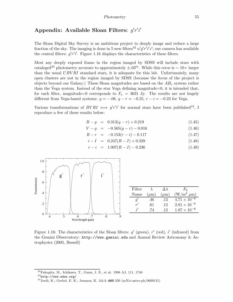
Photometry 55

Appendix: Available Sloan Filters: g′r′i′

The Sloan Digital Sky Survey is an ambitious project to deeply image and reduce a largefraction of the sky. The imaging is done in 5 new filters42 u′g′r′i′z′; our camera has availablethe central filters: g′r′i′. Figure 1.16 displays the characteristics of these filters.

Most any deeply exposed frame in the region imaged by SDSS will include stars withcataloged43 photometry accurate to approximately ±.03m. While this error is ∼ 10× largerthan the usual UBV RI standard stars, it is adequate for this lab. Unfortunately, manyopen clusters are not in the region imaged by SDSS (because the focus of the project isobjects beyond our Galaxy.) These Sloan magnitudes are based on the ABν system ratherthan the Vega system. Instead of the star Vega defining magnitude=0, it is intended that,for each filter, magnitude=0 corresponds to Fν = 3631 Jy. The results are not hugelydifferent from Vega-based systems: g = −.08, g − r = −0.25, r − i = −0.23 for Vega.

Various transformations of BV RI ⇐⇒ g′r′i′ for normal stars have been published44, Ireproduce a few of these results below:

B − g = 0.313(g − r) + 0.219 (1.45)

V − g = −0.565(g − r) − 0.016 (1.46)

R − r = −0.153(r − i) − 0.117 (1.47)

i − I = 0.247(R − I) + 0.329 (1.48)

r − i = 1.007(R − I) − 0.236 (1.49)

.4 .5 .6 .7 .8 .9

1.0

.8

.6

.4

.2

0

Wavelength ( m)

Tra

nsm

issi

on

g´ r´ i´

µ

Filter λ ∆λ F0

Name (µm) (µm) (W/m2 µm)

g′ .46 .13 4.71 × 10−8

r′ .61 .12 2.81 × 10−8

i′ .74 .12 1.87 × 10−8

Figure 1.16: The characteristics of the Sloan filters: g′ (green), r′ (red), i′ (infrared) fromthe Gemini Observatory: http://www.gemini.edu and Annual Review Astronomy & As-trophysics (2005, Bessell)

42Fukugita, M., Ichikawa, T., Gunn, J. E., et al. 1996 AJ, 111, 174843http://www.sdss.org/44Jordi, K.; Grebel, E. K.; Ammon, K. A&A 460 339 (arXiv:astro-ph/0609121)

56 Photometry

Appendix: ST-7E Camera

In June 2009 we ‘retired’ the old but fully functional SBIG ST-7E camera. I’ve dumped thespecifications for this camera in this Appendix as it is possible that it might be returnedto service. Flaws in the CCD are most evident in the bias frame45. Measurements on ourCCD shows that the difference between two bias frames shows an approximately normaldistribution (aside from the flaws) with a standard deviation ∼ 6 ADU. Also note that thesystem artificially introduces an offset of 100 into each pixel, so 2

3of the pixels in a bias

frame are expected in the range 100± 6 ADU. The ST-7 uses a thermoelectric cooler whichcan cool the CCD ∼ 30◦C below ambient temperature, reducing the dark currents by abouta factor of 10. The resulting dark currents are not negligible for exposures longer than afew minutes.

45Our CCD has a flaw at pixel (592, 194) which affects the entire 592 column

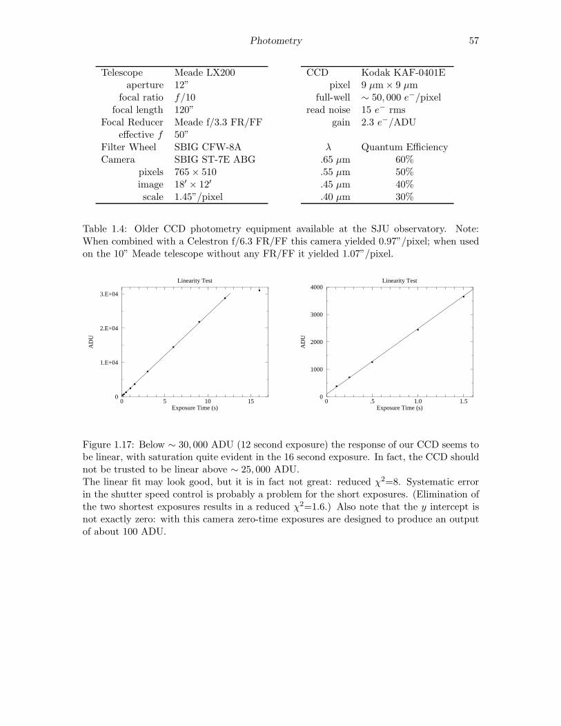
Photometry 57

Telescope Meade LX200aperture 12”

focal ratio f/10focal length 120”

Focal Reducer Meade f/3.3 FR/FFeffective f 50”

Filter Wheel SBIG CFW-8ACamera SBIG ST-7E ABG

pixels 765 × 510image 18′ × 12′

scale 1.45”/pixel

CCD Kodak KAF-0401Epixel 9 µm × 9 µm

full-well ∼ 50, 000 e−/pixelread noise 15 e− rms

gain 2.3 e−/ADU

λ Quantum Efficiency.65 µm 60%.55 µm 50%.45 µm 40%.40 µm 30%

Table 1.4: Older CCD photometry equipment available at the SJU observatory. Note:When combined with a Celestron f/6.3 FR/FF this camera yielded 0.97”/pixel; when usedon the 10” Meade telescope without any FR/FF it yielded 1.07”/pixel.

0 5 10 15

3.E+04

2.E+04

1.E+04

0

Linearity Test

Exposure Time (s)

AD

U

0 .5 1.0 1.5

4000

3000

2000

1000

0

Linearity Test

Exposure Time (s)

AD

U

Figure 1.17: Below ∼ 30, 000 ADU (12 second exposure) the response of our CCD seems tobe linear, with saturation quite evident in the 16 second exposure. In fact, the CCD shouldnot be trusted to be linear above ∼ 25, 000 ADU.The linear fit may look good, but it is in fact not great: reduced χ2=8. Systematic errorin the shutter speed control is probably a problem for the short exposures. (Elimination ofthe two shortest exposures results in a reduced χ2=1.6.) Also note that the y intercept isnot exactly zero: with this camera zero-time exposures are designed to produce an outputof about 100 ADU.

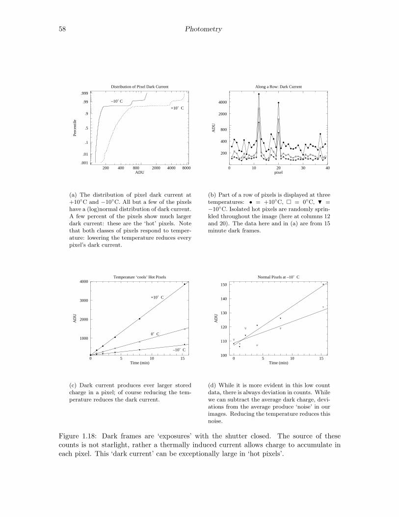
58 Photometry

200 400 800 2000 4000 8000

.999

.99

.9

.5

.1

.01

.001

Distribution of Pixel Dark Current

ADU

Perc

entil

e

–10˚ C

+10˚ C

(a) The distribution of pixel dark current at+10◦C and −10◦C. All but a few of the pixelshave a (log)normal distribution of dark current.A few percent of the pixels show much largerdark current: these are the ‘hot’ pixels. Notethat both classes of pixels respond to temper-ature: lowering the temperature reduces everypixel’s dark current.

0 10 20 30 40

4000

2000

800

400

200

Along a Row: Dark Current

pixel

AD

U

(b) Part of a row of pixels is displayed at threetemperatures: • = +10◦C, � = 0◦C, H =−10◦C. Isolated hot pixels are randomly sprin-kled throughout the image (here at columns 12and 20). The data here and in (a) are from 15minute dark frames.

0 5 10 15

4000

3000

2000

1000

Temperature ‘cools’ Hot Pixels

Time (min)

AD

U

0˚ C

+10˚ C

–10˚ C

(c) Dark current produces ever larger storedcharge in a pixel; of course reducing the tem-perature reduces the dark current.

0 5 10 15

150

140

130

120

110

100

Normal Pixels at –10˚ C

Time (min)

AD

U

(d) While it is more evident in this low countdata, there is always deviation in counts. Whilewe can subtract the average dark charge, devi-ations from the average produce ‘noise’ in ourimages. Reducing the temperature reduces thisnoise.

Figure 1.18: Dark frames are ‘exposures’ with the shutter closed. The source of thesecounts is not starlight, rather a thermally induced current allows charge to accumulate ineach pixel. This ‘dark current’ can be exceptionally large in ‘hot pixels’.