1

NONLINEAR MAPPING: APPROACHES BASED ON

OPTIMIZING AN INDEX OF CONTINUITY AND APPLYING CLASSICAL METRIC MDS TO

REVISED DISTANCESBy Ulas Akkucuk

& J. Douglas Carroll

Rutgers Business School – Newark and New Brunswick

2

Outline• Introduction• Nonlinear Mapping Algorithms

• Parametric Mapping Approach• ISOMAP Approach• Other Approaches

• Experimental Design and Methods• Error Levels• Evaluation of Mapping Performance• Problem of Similarity Transformations

• Results• Discussion and Future Direction

3

Introduction

• Problem: To determine a smaller set of variables necessary to account for a larger number of observed variables

• PCA and MDS are useful when relationship is linear

• Alternative approaches needed when the relationship is highly nonlinear

4

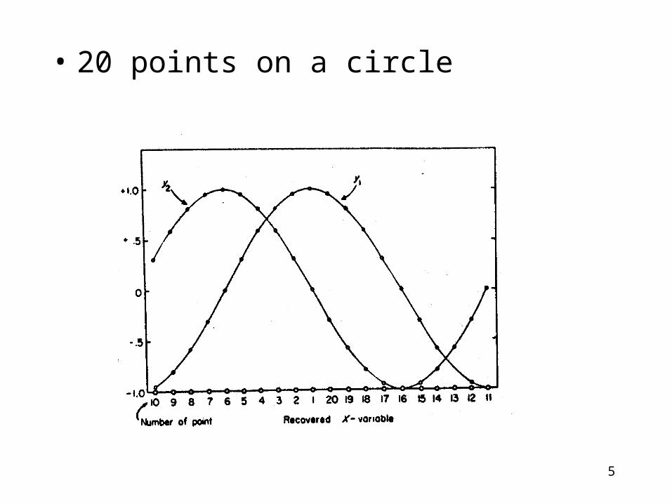
• Shepard and Carroll (1966)– Locally monotone analysis of proximities:

Nonmetric MDS treating large distances as missing• Worked well if the nonlinearities were not too severe (in

particular if the surface is not closed such as a circle or sphere)

– Optimization of an index of “continuity” or “smoothness”

• Incorporated into a computer program called “PARAMAP” and tested on various sets of data

5

• 20 points on a circle

6

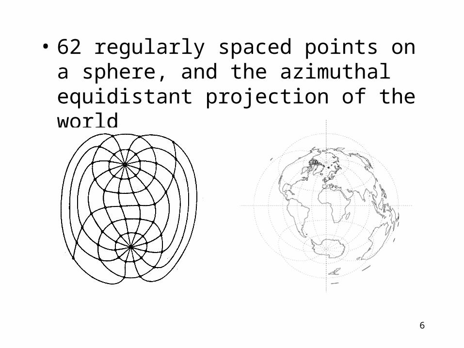
• 62 regularly spaced points on a sphere, and the azimuthal equidistant projection of the world

7

• 49 points regularly spaced on a torus embedded in four dimensions

8

• In all cases the local structure is preserved except points at which the shape is “cut open” or “punctured”

• Results were successful, but severe local minimum problem existed

• Addition of error to the regular spacing made the local minimum problem worse

• Current work is stimulated by two articles on nonlinear mapping (Tenenbaum, de Silva, & Langford, 2000; Roweis & Saul, 2000)

9

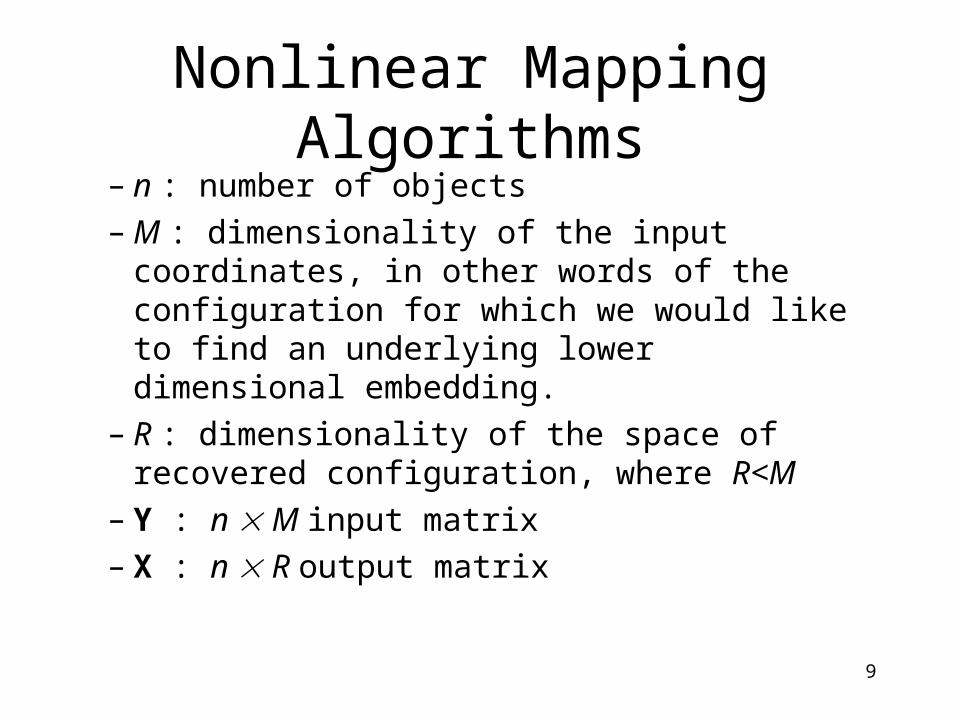
Nonlinear Mapping Algorithms– n : number of objects– M : dimensionality of the input coordinates, in

other words of the configuration for which we would like to find an underlying lower dimensional embedding.

– R : dimensionality of the space of recovered configuration, where R<M

– Y : n M input matrix– X : n R output matrix

10

– The distances between point i and point j in the input and output spaces respectively are calculated as:

[ ij ]D [ dij ]

jixxd

jiyy

R

rjririj

M

mjmimij

, ,)(

, ,)(

1

22

1

22

11

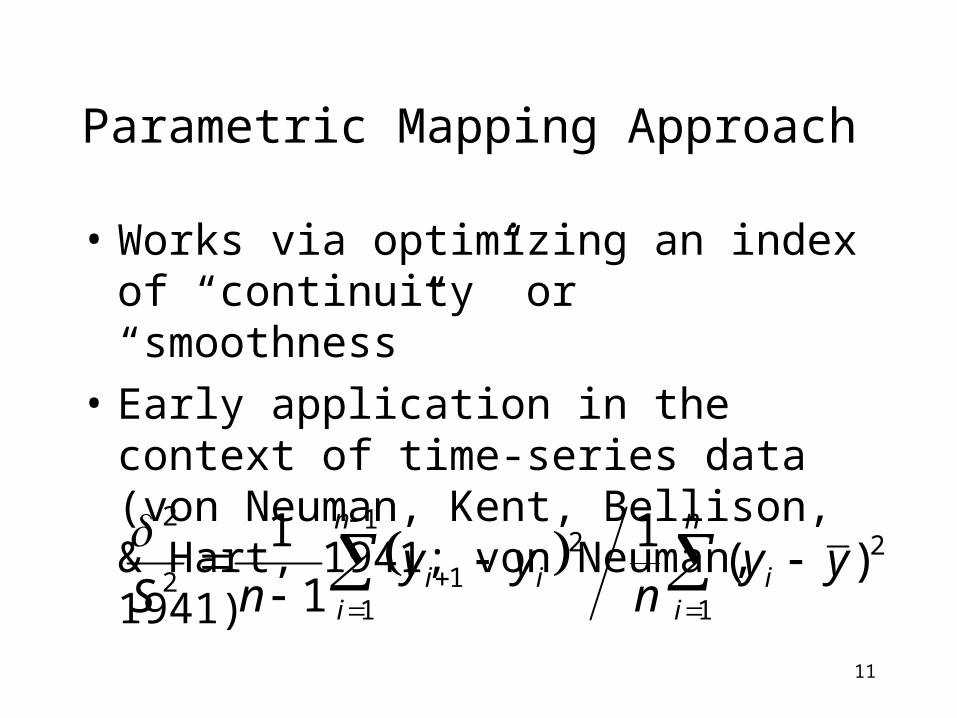
Parametric Mapping Approach

• Works via optimizing an index of “continuity” or “smoothness”

• Early application in the context of time-series data (von Neuman, Kent, Bellison, & Hart, 1941; von Neuman, 1941)

n

ii

n

iii yy

nyy

nS 1

21

1

212

2

)(1

1

1

12

• A more general expression for the numerator is:

• Generalizing to the multidimensional case we reach

21

1

2

1

1

n

i i

i

x

y

n

2

24

21

ji ji ijij

ij

dd

13

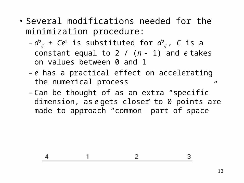
• Several modifications needed for the minimization procedure:– d2

ij + Ce2 is substituted for d2ij , C is a constant equal

to 2 / (n - 1) and e takes on values between 0 and 1

– e has a practical effect on accelerating the numerical process

– Can be thought of as an extra “specific” dimension, as e gets closer to 0 points are made to approach “common” part of space

14

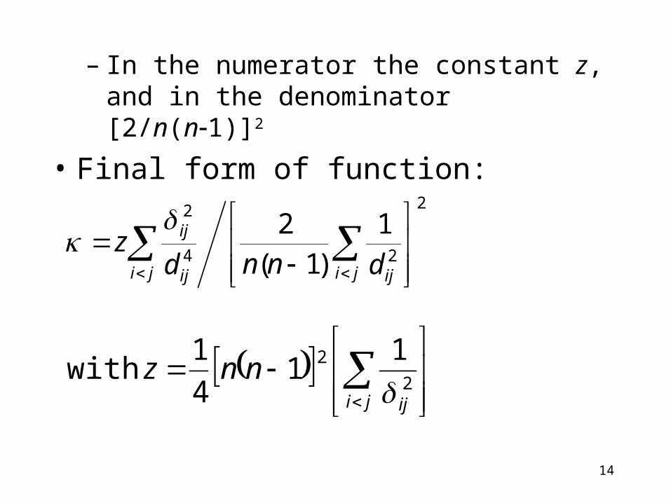
– In the numerator the constant z, and in the denominator [2/n(n1)]2

• Final form of function:

2

24

21

)1(

2

ji ji ijij

ij

dnndz

ji ij

nnz2

2 11

4

1with

15

• Implemented in C++ (GNU-GCC compiler)

• Program takes as input e, number of repetitions, dimensionality R to be recovered, and number of random starts or starting input configuration

• 200 iterations each for 100 different random configurations yields reasonable solutions

• Then this resulting best solution can be further fine tuned by performing more iterations

16

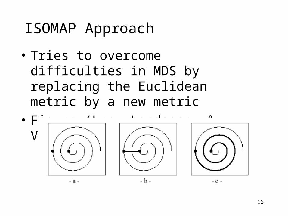
ISOMAP Approach

• Tries to overcome difficulties in MDS by replacing the Euclidean metric by a new metric

• Figure (Lee, Landasse, & Verleysen, 2002)

17

• To approximate the “geodesic” distances ISOMAP constructs a neighborhood graph that connects the closer points – This is done by connecting the k closest neighbors or

points that are close to each other by or less distance

• A shortest path procedure is then applied to the resulting matrix of modified distances

• Finally classical metric MDS is applied to obtain the configuration in the lower dimensionality

18

Other Approaches

• Nonmetric MDS: Minimizes a cost function

• Needed to implement locally monotone MDS approach of Shepard (Shepard & Carroll, 1966)

jiij

jiijij

d

dd

STRESS2

2ˆ

1

jiij

jiijij

dd

dd

STRESS2

2

)(

ˆ

2or

19

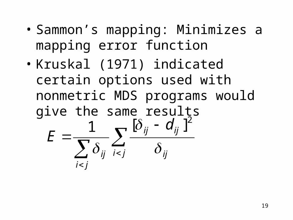
• Sammon’s mapping: Minimizes a mapping error function

• Kruskal (1971) indicated certain options used with nonmetric MDS programs would give the same results

ji ij

ijij

jiij

dE

2][1

20

• Multidimensional scaling by iterative majorization (Webb, 1995)

• Curvilinear Distance Analysis (CDA) (Lee et al., 2002), analogue of ISOMAP, omits the MDS step replacing it by a minimization step

• Self organizing map (SOM) (Kohonen 1990, 1995)

• Auto associative feedforward neural networks (AFN) (Baldi & Hornik, 1989; Kramer, 1991)

21

Experimental Design and Methods

• Primary focus: 62 located at the intersection of 5 equally spaced parallels and 12 equally spaced meridians

• Two types of error A and B – A: 0%, 10%, 20%– B: ±0.00, ±0.01, ±0.05, ±0.10, ±0.20

• Control points being irregularly spaced and being inside or outside the sphere respectively

22

23

• To evaluate mapping performance:We calculate “rate of agreement in local structure”abbreviated “agreement rate” or A– Similar to RAND index used to compare

partitions (Rand, 1971; Hubert & Arabie, 1985)

– Let ai stand for the number of points that are in the k-nearest neighbor list for point i in both X and Y. A will be equal to

knan

ii

1

24

1 2 3 4 5

2 1 1 2 1

3 4 4 3 2

1 2 3 4 5

4 3 2 1 3

5 4 4 5 4

k=2, Agreement rate = 2/10 or 20 %

Example of calculating agreement rate

25

• Problem of similarity transformations: We use standard software to rotate the different solutions into optimal congruence with a landmark solution (Rohlf & Slice 1989)

• We use the solution for the error free and regularly spaced sphere as the landmark

• We report also VAF

R

r

n

iir

R

r

n

iirir

x

xxVAF

1 1

2

1 1

2

)(

)ˆ(1

26

• The VAF results may not be very good

• Similarity transformation step is not enough

• An alternating algorithm is needed that reorders the points on each of the five parallels and then finds the optimal similarity transformation

• We also provide Shepard-like diagrams

27

(a) 0% Type A Error / 0.00 Type B Error

-0.20 -0.10 0.00 0.10 0.20

-0.20

-0.10

0.00

0.10

0.20

1

23 4

56

7891011

1213

14

15 16

17

18

19

20212223

24

2526

27

28

29

30

31

32333435

36

37

3839

40

41

42

43

444546

47

48

4950 51 52

535455

56575859

6061

62

(b) 0% Type A Error / 0.01 Type B ErrorVAF = 0.47

-0.20 -0.10 0.00 0.10 0.20

-0.20

-0.10

0.00

0.10

0.20

12

3 4 5 678

91011

1213

14

1516 17 18

19

20

21

2223

24

25

26

27 28 29 30

31

32

33 34

35

36

37

38

39 40 4142

43

44

45

4647

48

49

5051 52 53 54

5556

575859

6061

62

Why similarity transformation is not enough?

28

Results• Agreement rate for the regularly spaced and

errorless sphere 82.9%, k=5

• Over 1000 randomizations of the solution: Average, and standard deviation of the agreement rate 8.1% and 1.9% respectively. Minimum and maximum are 3.5% and 16.7%

29

-0.25

-0.2

-0.15

-0.1

-0.05

0

0.05

0.1

0.15

0.2

0.25

-0.25 -0.2 -0.15 -0.1 -0.05 0 0.05 0.1 0.15 0.2 0.25

30

• We can use Chebychev’s inequality stated as:

• 82.9 is about 40 standard deviations away from the mean, an upper bound of the probability that this event happens by chance is 1/402 or 0.000625, very low!

2

1)(

kkZP

31

(a) 0% Type A Error / 0.00 Type B Error

-0.20 -0.10 0.00 0.10 0.20

-0.20

-0.10

0.00

0.10

0.20

1

23 4

56

7891011

1213

14

15 16

17

18

19

20212223

24

2526

27

28

29

30

31

32333435

36

37

3839

40

41

42

43

444546

47

48

4950 51 52

535455

56575859

6061

62

(b) 0% Type A Error / 0.01 Type B ErrorVAF = 0.47

-0.20 -0.10 0.00 0.10 0.20

-0.20

-0.10

0.00

0.10

0.20

12

3 4 5 678

91011

1213

14

1516 17 18

19

20

21

2223

24

25

26

27 28 29 30

31

32

33 34

35

36

37

38

39 40 4142

43

44

45

4647

48

49

5051 52 53 54

5556

575859

6061

62

(c) 0% Type A Error / 0.05 Type B ErrorVAF = 0.42

-0.20 -0.10 0.00 0.10 0.20

-0.20

-0.10

0.00

0.10

0.20

1

2 345

678

91011

12 13

14 15

16

17

18

1920

21

22

23

2425

26 27

2829

30

31

32

33

34

35

36 37

3839

40

41

42

4344

45

46

47

48 49

5051

5253

54555657

5859

60 61

62

(d) 0% Type A Error / 0.10 Type B ErrorVAF = 0.63

-0.20 -0.10 0.00 0.10 0.20

-0.20

-0.10

0.00

0.10

0.20

1

2 345

6789

101112

13

1415

16

17

18192021

22

23

24

25

26

27

28

29

30

31323334

35

36

37

3839 40

41

42

43444546

47

48

4950 5152

53

5455

56575859

6061

62

(a) (b)

(c) (d)

32

(e) 0% Type A Error / 0.20 Type B ErrorVAF=0.23

-0.20 -0.10 0.00 0.10 0.20-0.20

-0.10

0.00

0.10

0.20

1

2 34

56789

1011

1213

1415

16

17

1819

2021

22

2324

25

26

2728

29

30

31

32

33

34 35 36 37

38

39

40

4142

43

44

45

46 47 48 49

505152535455

56575859 6061

62

(f) 10% Type A Error / 0.00 Type B ErrorVAF = 0.61

-0.20 -0.10 0.00 0.10 0.20

-0.20

-0.10

0.00

0.10

0.20

1

2 34

5678

9

10

1112

13

14

1516

17

181920

212223

2425

2627

28

29

3031

323334

3536

37

38

39

40

41

4243

44

454647

4849

50

5152

5354

555657

58

59

6061 62

(g) 10% Type A Error / 0.01 Type B ErrorVAF = 0.33

-0.20 -0.10 0.00 0.10 0.20

-0.20

-0.10

0.00

0.10

0.20

12

34

5 6 7

8

9

101112

13

14 15

16 17 1819 20

2122

23

24

25

26 27 2829

3031

3233

34

35

36

37

38 39

40

41

42

43

44

45

4647

4849

505152

5354

555657 58

5960

61

62

(h) 10% Type A Error / 0.05 Type B ErrorVAF = 0.62

-0.20 -0.10 0.00 0.10 0.20

-0.20

-0.10

0.00

0.10

0.20

1

2 34

56

789

10

1112

13

14

15

16

17

1819

20212223

24

25

26 2728

29

30

3132

33343536

37

38

39

40

4142

4344

454647

4849

50 5152 5354

555657

5859

606162

(e) (f)

(g) (h)

33

(i) 10% Type A Error / 0.10 Type B ErrorVAF = 0.49

-0.20 -0.10 0.00 0.10 0.20

-0.20

-0.10

0.00

0.10

0.20

1

23

456

7

8

9

101112

1314

1516 17

1819

20

21222324

252627

28

29

3031

32

3334353637

38

39

40

41

42

43

4445

464748

49

50

5152

5354

5556

57

5859

60

61

62

(j) 10% Type A Error / 0.20 Type B ErrorVAF = 0.27

-0.20 -0.10 0.00 0.10 0.20

-0.20

-0.10

0.00

0.10

0.20

12 3

4

56 7

8

9

10

1112 13

1415

16 171819

20

2122

23

24

25

26 27 2829

3031

3233

34

35

36

37

38 39

40

41

42

43

4445

4647

4849

505152

5354

5556

5758

5960

61

62

(k) 20% Type A Error / 0.00 Type B ErrorVAF = 0.37

-0.20 -0.10 0.00 0.10 0.20

-0.20

-0.10

0.00

0.10

0.20

12

3

4

5

67

8

910

111213

1415

1617

1819

20

21

22

2324

25

2627

2829

30

31

32

33

34

35

36

37

38

3940

4142

43

4445

4647

48

4950 51 5253

54

55

5657

5859

60

6162

(l) 20% Type A Error / 0.01 Type B ErrorVAF = 0.42

-0.20 -0.10 0.00 0.10 0.20

-0.20

-0.10

0.00

0.10

0.20

12

3

45 6

78

9

10

1112 13

14

15

1617

18

19

20

2122

23 24

25

2627

28

2930

31

32

33

34

35

36

37

38

3940

41

4243

4445

46

47

48

49

50

51

5253 54

55

56

57

5859

6061

62

(i) (j)

(k) (l)

34

(m) 20% Type A Error / 0.05 Type B ErrorVAF = 0.34

-0.20 -0.10 0.00 0.10 0.20

-0.20

-0.10

0.00

0.10

0.20

12

3

45

6

7

89

10

11

12 13

1415

1617

18 19

20

2122 2324

25

26 27

28

2930

31

32

33

34

35

36

37

383940

41

4243

44

4546

47

48

49

50

51

52

53 54

5556

57

5859

60 61

62

(n) 20% Type A Error / 0.10 Type B ErrorVAF = 0.37

-0.20 -0.10 0.00 0.10 0.20

-0.20

-0.10

0.00

0.10

0.20

12

3

45

6

7

89

10

11

12

13

14

15

16

17

18 19

20

212223

24

25

26

27

28

2930

31

32

3334

353637

38

3940 41

42

43

4445

46474849

50

51

52

53

54

55

5657

58

596061

62

(o) 20% Type A Error / 0.20 Type B ErrorVAF = 0.36

-0.20 -0.10 0.00 0.10 0.20

-0.20

-0.10

0.00

0.10

0.20

12

3

4 5

6

789

10

11

12

13

14

15

16

17

1819

20

21222324

25

26

27

28

2930

31

3233

34

35

3637

38

39 4041 42

43

4445

46

4748

49 50 5152

53

5455

56

5758

59

60

61 62

(m) (n)

(o)

35

36

(a) 0% Type A Error / 0.00 Type B Error

-0.20 -0.10 0.00 0.10 0.20

-0.20

-0.10

0.00

0.10

0.20

1

23 4

56

7891011

1213

14

15 16

17

18

19

20212223

24

2526

27

28

29

30

31

32333435

36

37

3839

40

41

42

43

444546

47

48

4950 51 52

535455

56575859

6061

62

A=48.1 %

A=82.9%

ISOMAP

PARAMAP

37

(a)

0

0.2

0.4

0.6

0.8

1

1.2

1.4

0 0.02 0.04 0.06 0.08 0.1 0.12

recovered distances

orig

inal

dis

tanc

es(b)

0

0.2

0.4

0.6

0.8

1

1.2

1.4

0 0.02 0.04 0.06 0.08 0.1 0.12

recovered distances

orig

inal

dis

tanc

es

(c)

0

0.2

0.4

0.6

0.8

1

1.2

1.4

0 0.1 0.2 0.3 0.4 0.5 0.6 0.7 0.8 0.9

recovered distances

orig

inal

dis

tanc

es

Shepard-like Diagrams

38Agreement rate=ISOMAP 59.7%, PARAMAP 70.5%

SWISS Roll Data – 130 points

39

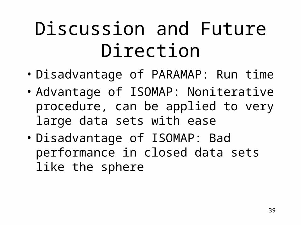
Discussion and Future Direction

• Disadvantage of PARAMAP: Run time

• Advantage of ISOMAP: Noniterative procedure, can be applied to very large data sets with ease

• Disadvantage of ISOMAP: Bad performance in closed data sets like the sphere

40

• Improvements in computational efficiency of PARAMAP should be explored:– Use of a conjugate gradient algorithm instead of straight

gradient algorithm – Use of conjugate gradient with restarts algorithm– Possible combination of straight gradient and conjugate

gradient approaches

• Improvements that could both benefit ISOMAP and PARAMAP:– A wise selection of landmarks and an interpolation or

extrapolation scheme to recover the rest of the data