1

IX. Explaining Relative Prices

2

Explaining Relative Prices

1. CAPM – Capital Asset Pricing Model

2. Non Standard Forms of the CAPM

3. APT – Arbitrage Pricing Theory

3

Assumptions behind the CAPM1. No transaction costs

2. Assets are infinitely divisible

3. No personal taxes

4. Price Takers

5. Investors look only at expected return and variances of their portfolio

6. Unlimited short sales

7. Unlimited lending and borrowing at the riskless Rate

8. Homogenous Expectations about time horizon

9. Homogenous expectations of expected return, variance, and covariance

10. All assets are marketable

4

Sharpe – Lintner – Mossine (CAPM)

Two Approaches to deriving

1. Economic intuition

2. Rigorous analysis

5

6

7

A more rigorous proof

P

FP RR

Max

Lintner Equation

NXXRR

kii

ikikkFk1

2

1

k F k k k k k i k k i i

N

ii k

R R E X R R R R X R R R R

8

1k F k k i i ii

NR R E R R X R R

Homogenous Expectations

kMFk RR

9

kMFk RR

Must hold for all securities and portfolios

2MFM RR

2M

FM RR

FMM

kMFk RRRR

2

FMkFk RRRR

10

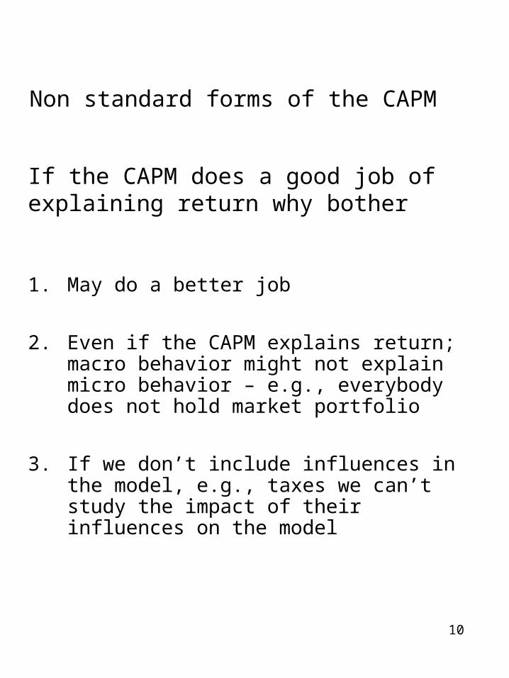
Non standard forms of the CAPM

1. May do a better job

2. Even if the CAPM explains return; macro behavior might not explain micro behavior – e.g., everybody does not hold market portfolio

3. If we don’t include influences in the model, e.g., taxes we can’t study the impact of their influences on the model

If the CAPM does a good job of explaining return why bother

11

Modification of assumptions

1. Short sales

2. Riskless lending and borrowing

3. Personal taxes

4. Non marketable assets

5. Heterogeneous expectations

6. Non price taking behavior

7. Multi period analysis

8. Consumption CAPM

Rolls critique

12

Short Sales

Since under the standard CAPM nobody short sells in equilibrium

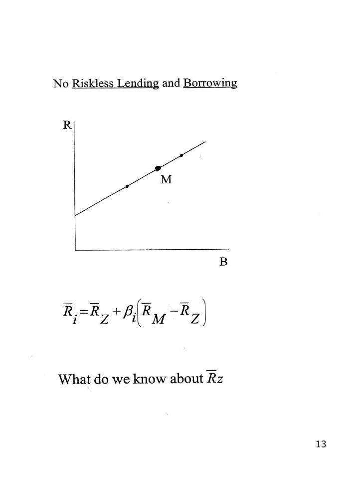
13

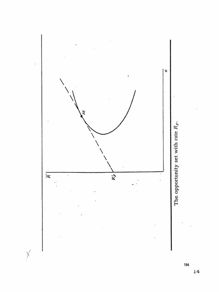
14

15

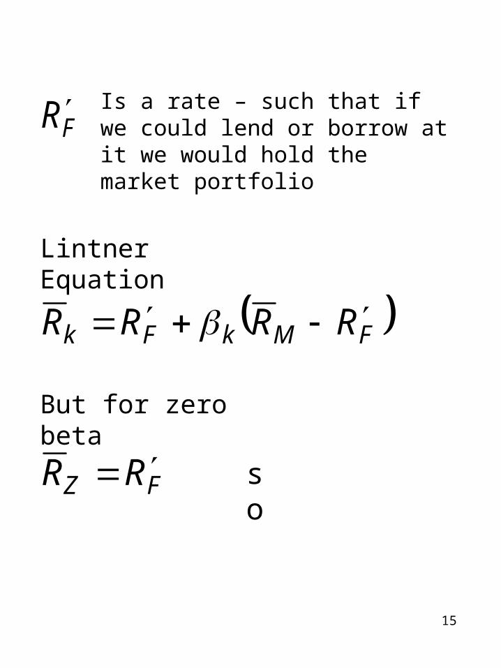
FRIs a rate – such that if we could lend or borrow at it we would hold the market portfolio

Lintner Equation

FMkFk RRRR

But for zero beta

FZ RR so

16

17

MZ RR by convexity of efficient frontier

01 22222 MZZZC XX

0222 2222

MZMZZZ

C XXdX

d

22

2

ZM

MZX

Prof that return on global minimum

variance portfolioGR Rz

18

ZX is greater than 0 and smaller than 1

Global minimum variance involves positive investment in market and zero beta portfolios and therefore, expected return must be in between.

19

20

21

22

23

24

Non Marketable Assets

CAPM

2

cov

m

mii

RR

mim

FmFi RR

RRRR cov

2

With nonmarketable assets (H)

Hi

m

Hmi

Hmm

Hm

FmFi RRRR

RR

RRRR covcov

cov2

Price of risk * amount of risk

25

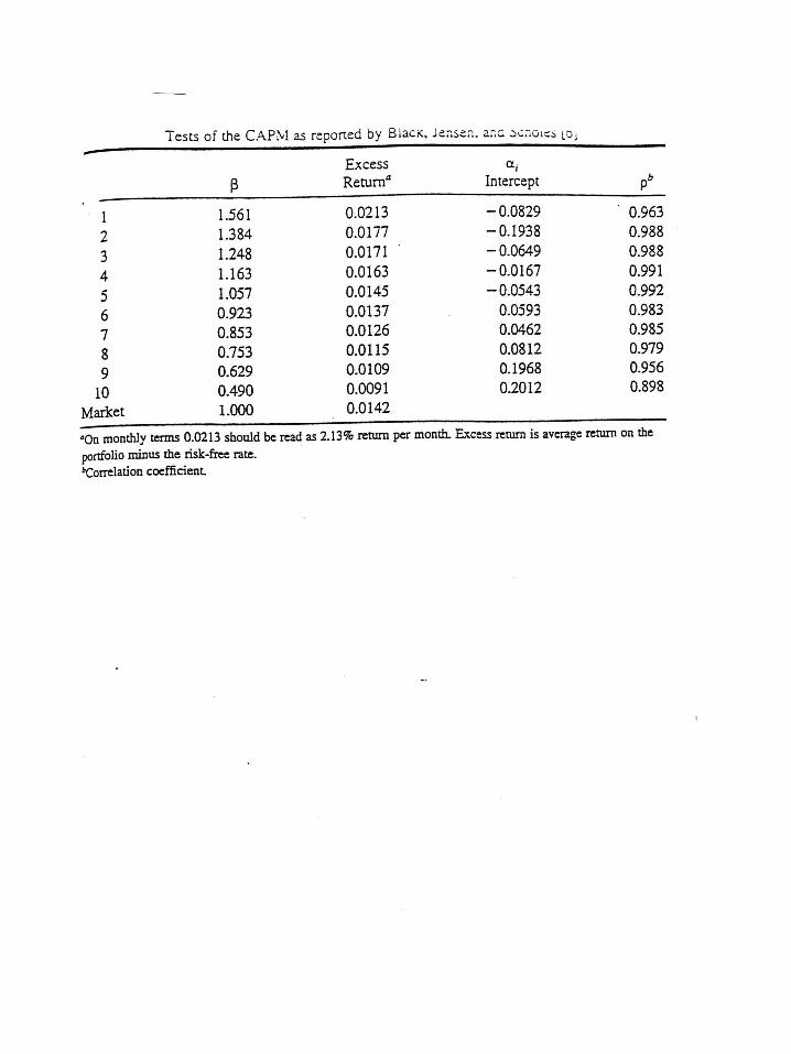
Test of Equilibrium Models

FMiFi RRRR Expectations (1)

Test with realizations – expectations are an average and on the whole correct

Market Model

itmtiiit eRR

miii RR

itmmtiii eRRRR

Substitution

itFmtiFit eRRRR

26

27

28

itMtiiZit eRRR 1

itMtiiFiit eRRR 1

1i Z F iR R

29

30

31

Fama and Mac Beth

iteitittttit SR 32

210

1.

2.

3.

03 tE

02 tE

01 tE

Auto correlation of , , and ,t0 t1 0

FR0 FM RR 1

32

33

34

35

Rolls Critique

Mathematically can show for any efficient portfolio

ZPPkPZPk RRRR

“Unfortunately it has never been subject to an unambiguous empirical test. There is considerable doubt…that it will be.”

36

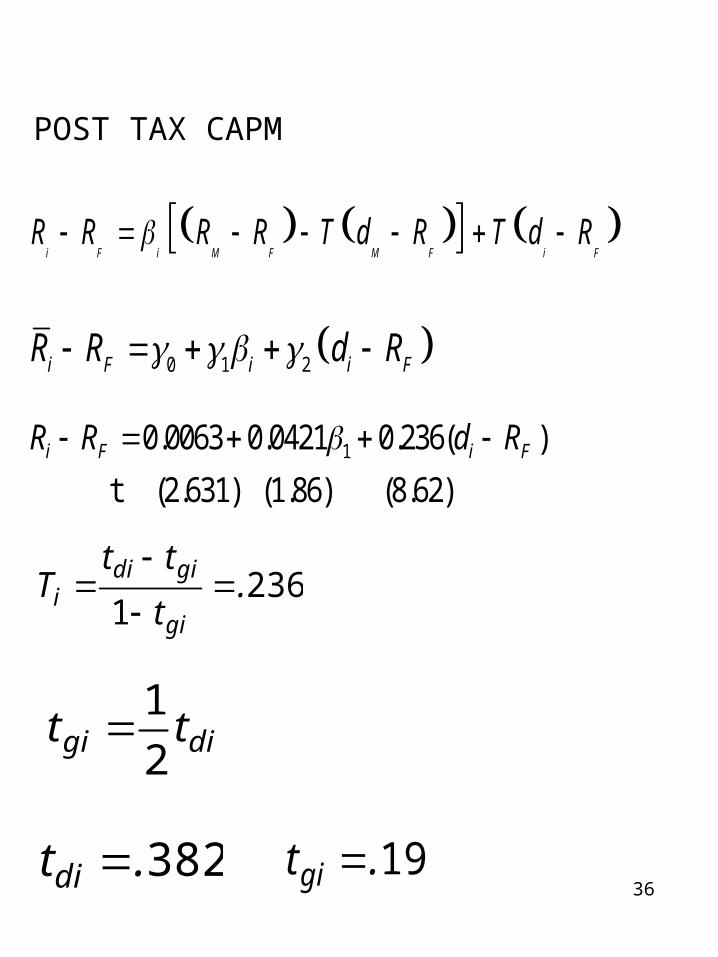
POST TAX CAPM

i F i M F M F i FR R R R T d R T d R

0 1 2i F i i FR R d R

2361

.t

ttT

gi

gidii

digi tt2

1

382.tdi 19.tgi

10.0063 0.0421 0.236( )

t (2.631) (1.86) (8.62)i F i FR R d R