1 iterative methods for non-linear systems of equations

1Iterative Method s for Non-Linear

Systems of EquationsA non-linear system of equations is a concept almost too abstract to be useful, because it covers

an extremely wide variety of problems . Nevertheless in this chapter we will mainly look at “generic”

methods for such systems. This means that every method discussed may take a good deal of fine-

tuning before it will really perform satisfactorily for a given non-linear system of equations.

Given: function F : D ⊂ Rn 7→ Rn, n ∈ N

mPossible meaning: Availability of a procedure function y=F(x) evaluating F

Sought: solution of non-linear equation F (x) = 0

Note: F : D ⊂ Rn 7→ R

n ↔ “same number of equations and unknowns”

In general no existence & uniqueness of solutions

GradinaruD-MATHp. 181.1

Num.Meth.Phys.

1.1 Iterative method s

Remark 1.1.1 (Necessity of iterative approximation).

Gaussian elimination provides an algorithm that, if carried out in exact arithmetic, computes the so-

lution of a linear system of equations with a finite number of elementary operations. However, linear

systems of equations represent an exceptional case, because it is hardly ever possible to solve gen-

eral systems of non-linear equations using only finitely many elementary operations. Certainly this is

the case whenever irrational numbers are involved.△ GradinaruD-MATH

p. 191.1Num.Meth.Phys.

'

&

$

%

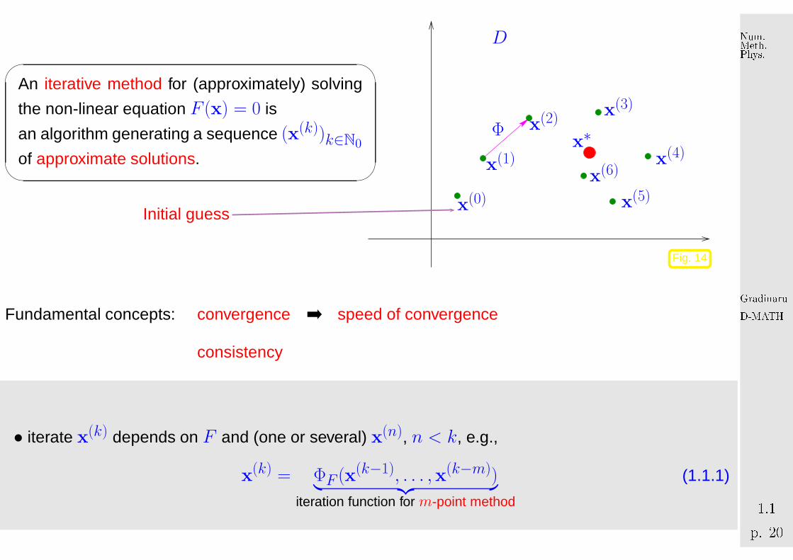
An iterative method for (approximately) solving

the non-linear equation F (x) = 0 is

an algorithm generating a sequence (x(k))k∈N0

of approximate solutions.

Initial guess x(0)

x(1)

x(2) x(3)

x(4)

x(5)x(6)

x∗Φ

D

Fig. 14

Fundamental concepts: convergence ➡ speed of convergence

consistency

• iterate x(k) depends on F and (one or several) x(n), n < k, e.g.,

x(k) = ΦF (x(k−1), . . . ,x(k−m))︸︷︷︸iteration function for m-point method

(1.1.1)


Num.Meth.Phys.

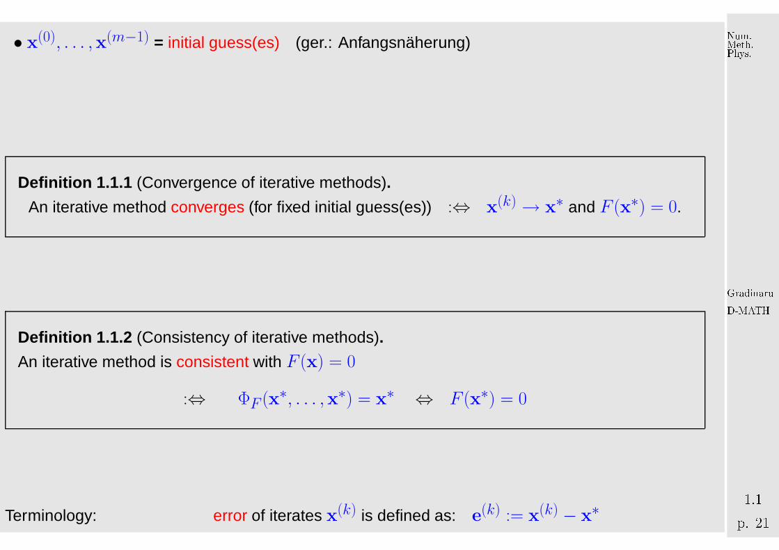
• x(0), . . . ,x(m−1) = initial guess(es) (ger.: Anfangsnäherung)

Defin ition 1.1.1 (Convergence of iterative methods).

An iterative method converges (for fixed initial guess(es)) :⇔ x(k) → x∗ and F (x∗) = 0.

Defin ition 1.1.2 (Consistency of iterative methods).

An iterative method is consistent with F (x) = 0

:⇔ ΦF (x∗, . . . ,x∗) = x∗ ⇔ F (x∗) = 0

Terminology: error of iterates x(k) is defined as: e(k) := x(k) − x∗


Num.Meth.Phys.

Defin ition 1.1.3 (Local and global convergence).

An iterative method converges locally to x∗ ∈ Rn, if there is a neighborhood U ⊂ D of x∗,such that

x(0), . . . ,x(m−1) ∈ U ⇒ x(k) well defined ∧ limk→∞

x(k) = x∗

for the sequences (x(k))k∈N0of iterates.

If U = D, the iterative method is globally convergent.

local convergence �

(Only initial guesses “sufficiently close” to x∗ guar-

antee convergence.)

x∗

D

U

Fig. 15


Num.Meth.Phys.

Goal: Find iterative methods that converge (locally) to a solution of F (x) = 0.

Two general questions: How to measure the speed of convergence?

When to terminate the iteration?

1.1.1 Speed of convergence

Here and in the sequel, ‖·‖ designates a generic vector norm, see Def. 1.1.9. Any occurring matrix

norm is indiuced by this vector norm, see Def. 1.1.12.

It is important to be aware which statements depend on the choice of norm and which do not!

“Speed of convergence” ↔ decrease of norm (see Def. 1.1.9) of iteration error


Num.Meth.Phys.

Defin ition 1.1.4 (Linear convergence).

A sequence x(k), k = 0, 1, 2, . . ., in Rn converges linearly to x∗ ∈ Rn, if

∃L < 1:∥∥∥x(k+1) − x∗

∥∥∥ ≤ L∥∥∥x(k) − x∗

∥∥∥ ∀k ∈ N0 .

Terminology: least upper bound for L gives the rate of convergence

Remark 1.1.2 (Impact of choice of norm).

Fact of convergence of iteration is independent of choice of normFact of linear convergence depends on choice of normRate of linear convergence depends on choice of norm

]

Norms provide tools for measuring errors. Recall from linear algebra and calculus:


Num.Meth.Phys.

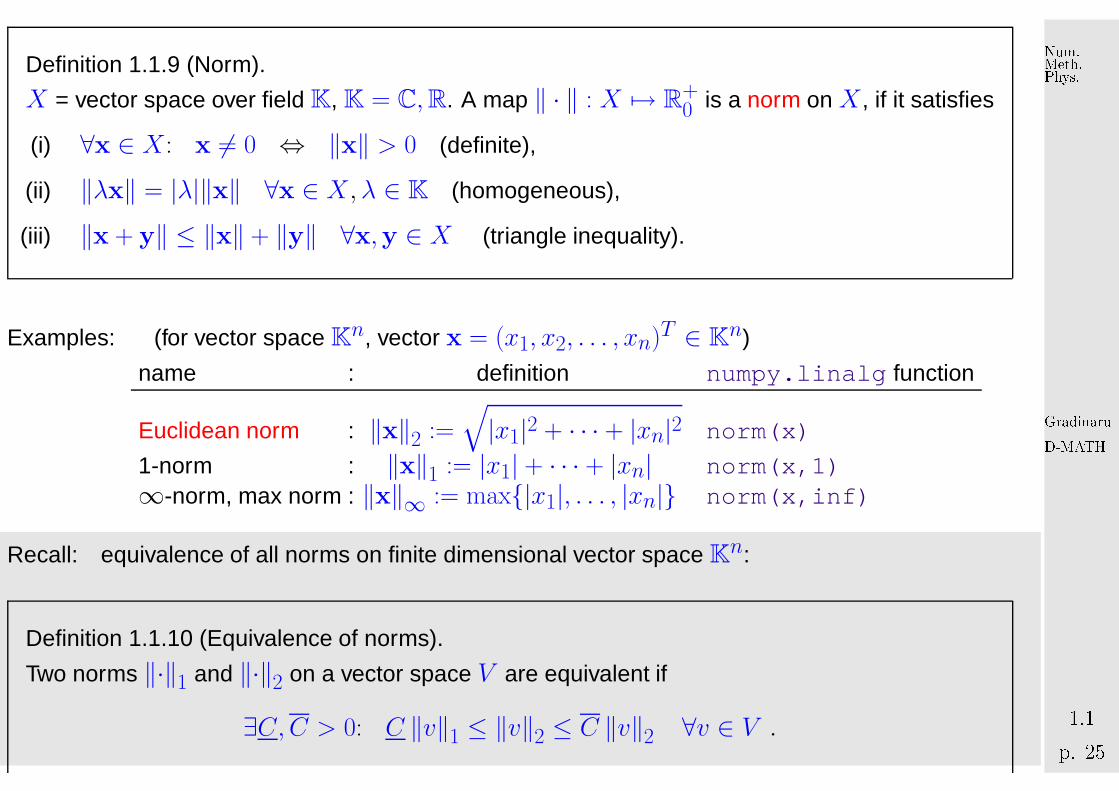
Definition 1.1.9 (Norm).

X = vector space over field K, K = C,R. A map ‖ · ‖ : X 7→ R+0 is a norm on X , if it satisfies

(i) ∀x ∈ X : x 6= 0 ⇔ ‖x‖ > 0 (definite),

(ii) ‖λx‖ = |λ|‖x‖ ∀x ∈ X,λ ∈ K (homogeneous),

(iii) ‖x + y‖ ≤ ‖x‖ + ‖y‖ ∀x,y ∈ X (triangle inequality).

Examples: (for vector space Kn, vector x = (x1, x2, . . . , xn)T ∈ Kn)

name : definition numpy.linalg function

Euclidean norm : ‖x‖2 :=√|x1|2 + · · · + |xn|2 norm(x)

1-norm : ‖x‖1 := |x1| + · · · + |xn| norm(x,1)∞-norm, max norm : ‖x‖∞ := max{|x1|, . . . , |xn|} norm(x,inf)

Recall: equivalence of all norms on finite dimensional vector space Kn:

Definition 1.1.10 (Equivalence of norms).

Two norms ‖·‖1 and ‖·‖2 on a vector space V are equivalent if

∃C,C > 0: C ‖v‖1 ≤ ‖v‖2 ≤ C ‖v‖2 ∀v ∈ V .


Num.Meth.Phys.

'

&

$

%

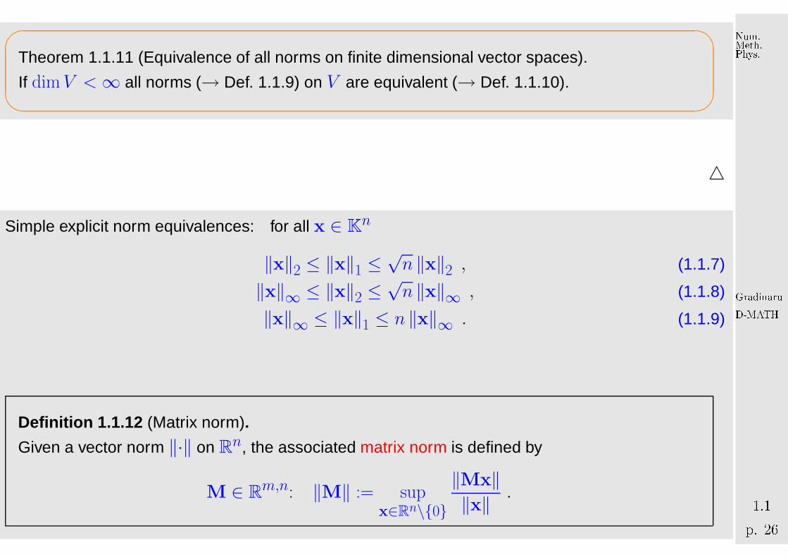
Theorem 1.1.11 (Equivalence of all norms on finite dimensional vector spaces).

If dimV <∞ all norms (→ Def. 1.1.9) on V are equivalent (→ Def. 1.1.10).

△

Simple explicit norm equivalences: for all x ∈ Kn

‖x‖2 ≤ ‖x‖1 ≤√n ‖x‖2 , (1.1.7)

‖x‖∞ ≤ ‖x‖2 ≤√n ‖x‖∞ , (1.1.8)

‖x‖∞ ≤ ‖x‖1 ≤ n ‖x‖∞ . (1.1.9)

Defin ition 1.1.12 (Matrix norm).

Given a vector norm ‖·‖ on Rn, the associated matrix norm is defined by

M ∈ Rm,n: ‖M‖ := sup

x∈Rn\{0}

‖Mx‖‖x‖ .


Num.Meth.Phys.

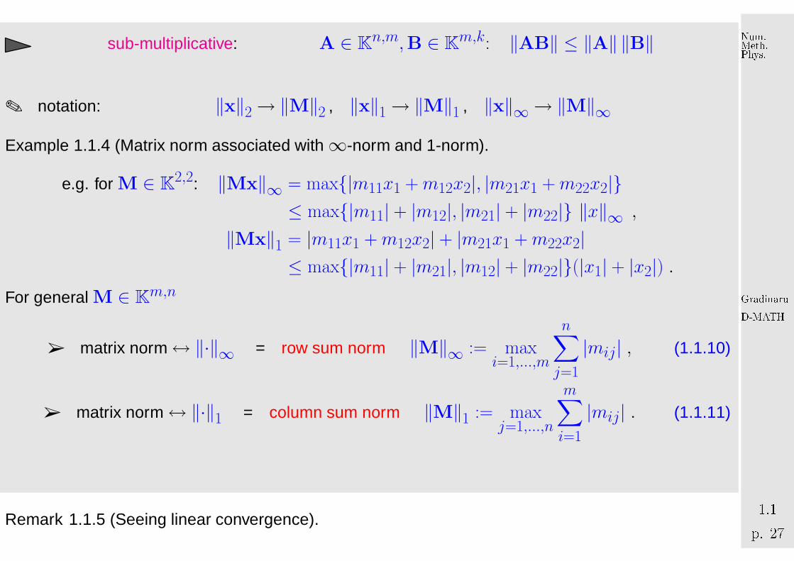
sub-multiplicative: A ∈ Kn,m,B ∈ K

m,k: ‖AB‖ ≤ ‖A‖ ‖B‖

✎ notation: ‖x‖2→ ‖M‖2 , ‖x‖1→ ‖M‖1 , ‖x‖∞→ ‖M‖∞Example 1.1.4 (Matrix norm associated with∞-norm and 1-norm).

e.g. for M ∈ K2,2: ‖Mx‖∞ = max{|m11x1 +m12x2|, |m21x1 +m22x2|}

≤ max{|m11| + |m12|, |m21| + |m22|} ‖x‖∞ ,

‖Mx‖1 = |m11x1 +m12x2| + |m21x1 +m22x2|≤ max{|m11| + |m21|, |m12| + |m22|}(|x1| + |x2|) .

For general M ∈ Km,n

➢ matrix norm↔ ‖·‖∞ = row sum norm ‖M‖∞ := maxi=1,...,m

n∑

j=1

|mij| , (1.1.10)

➢ matrix norm↔ ‖·‖1 = column sum norm ‖M‖1 := maxj=1,...,n

m∑

i=1

|mij| . (1.1.11)

3

Remark 1.1.5 (Seeing linear convergence).


Num.Meth.Phys.

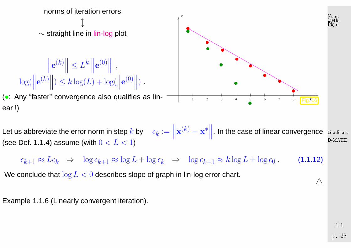
norms of iteration errors

l∼ straight line in lin-log plot

∥∥∥e(k)∥∥∥ ≤ Lk

∥∥∥e(0)∥∥∥ ,

log(∥∥∥e(k)

∥∥∥) ≤ k log(L) + log(∥∥∥e(0)

∥∥∥) .

(•: Any “faster” convergence also qualifies as lin-

ear !)1 2 3 4 5 6 7 8 k

e

Fig. 16

Let us abbreviate the error norm in step k by ǫk :=∥∥∥x(k) − x∗

∥∥∥. In the case of linear convergence

(see Def. 1.1.4) assume (with 0 < L < 1)

ǫk+1 ≈ Lǫk ⇒ log ǫk+1 ≈ logL + log ǫk ⇒ log ǫk+1 ≈ k logL + log ǫ0 . (1.1.12)

We conclude that logL < 0 describes slope of graph in lin-log error chart.△

Example 1.1.6 (Linearly convergent iteration).


Num.Meth.Phys.

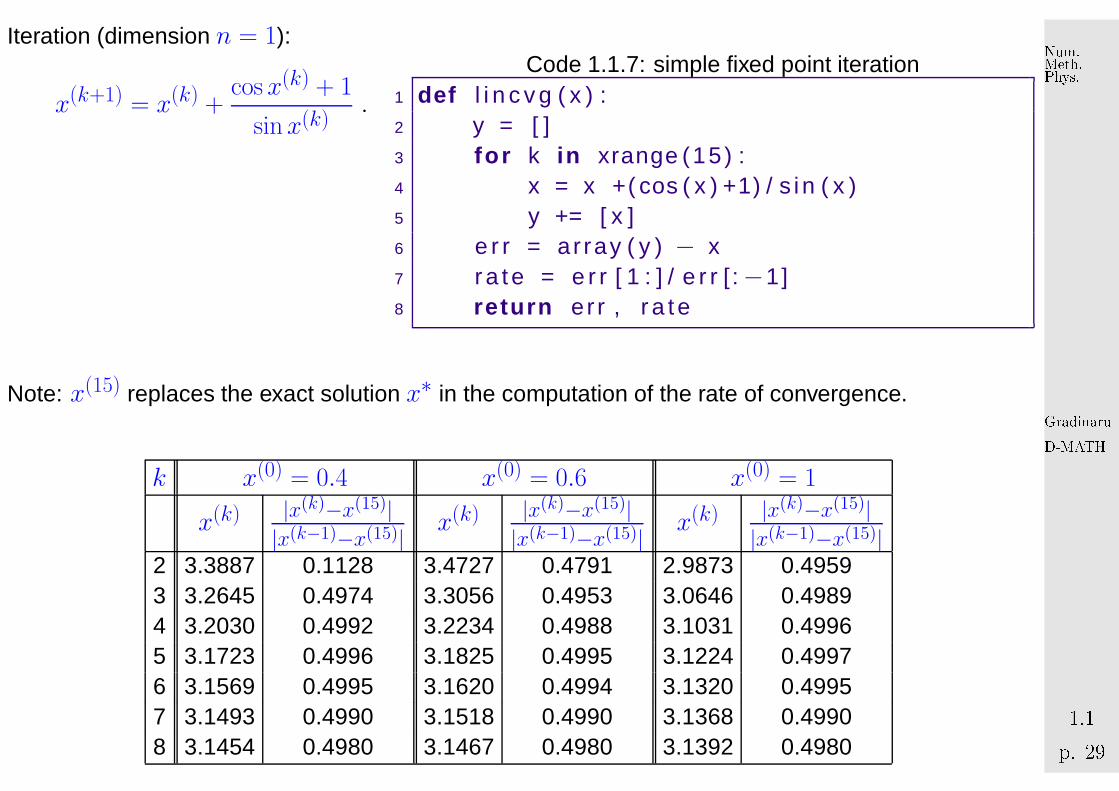
Iteration (dimension n = 1):

x(k+1) = x(k) +cos x(k) + 1

sinx(k).

Code 1.1.7: simple fixed point iteration1 def l i n c v g ( x ) :2 y = [ ]3 f o r k i n xrange (15) :4 x = x +( cos ( x ) +1) / s i n ( x )5 y += [ x ]6 e r r = ar ray ( y ) − x7 r a te = e r r [ 1 : ] / e r r [ :−1]8 r et u r n er r , r a te

Note: x(15) replaces the exact solution x∗ in the computation of the rate of convergence.

k x(0) = 0.4 x(0) = 0.6 x(0) = 1

x(k) |x(k)−x(15)||x(k−1)−x(15)| x(k) |x(k)−x(15)|

|x(k−1)−x(15)| x(k) |x(k)−x(15)||x(k−1)−x(15)|

2 3.3887 0.1128 3.4727 0.4791 2.9873 0.49593 3.2645 0.4974 3.3056 0.4953 3.0646 0.49894 3.2030 0.4992 3.2234 0.4988 3.1031 0.49965 3.1723 0.4996 3.1825 0.4995 3.1224 0.49976 3.1569 0.4995 3.1620 0.4994 3.1320 0.49957 3.1493 0.4990 3.1518 0.4990 3.1368 0.49908 3.1454 0.4980 3.1467 0.4980 3.1392 0.4980


Num.Meth.Phys.

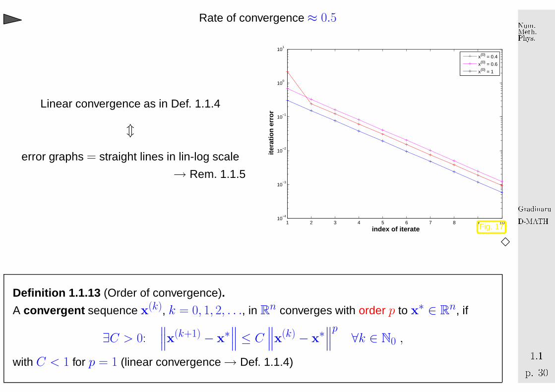
Rate of convergence≈ 0.5

Linear convergence as in Def. 1.1.4

m

error graphs = straight lines in lin-log scale

→ Rem. 1.1.5

1 2 3 4 5 6 7 8 9 1010

−4

10−3

10−2

10−1

100

101

index of iterate

iter

atio

n er

ror

x(0) = 0.4

x(0) = 0.6

x(0) = 1

Fig. 17

3

Defin ition 1.1.13 (Order of convergence).

A convergent sequence x(k), k = 0, 1, 2, . . ., in Rn converges with order p to x∗ ∈ R

n, if

∃C > 0:∥∥∥x(k+1) − x∗

∥∥∥ ≤ C∥∥∥x(k) − x∗

∥∥∥p∀k ∈ N0 ,

with C < 1 for p = 1 (linear convergence→ Def. 1.1.4)


Num.Meth.Phys.

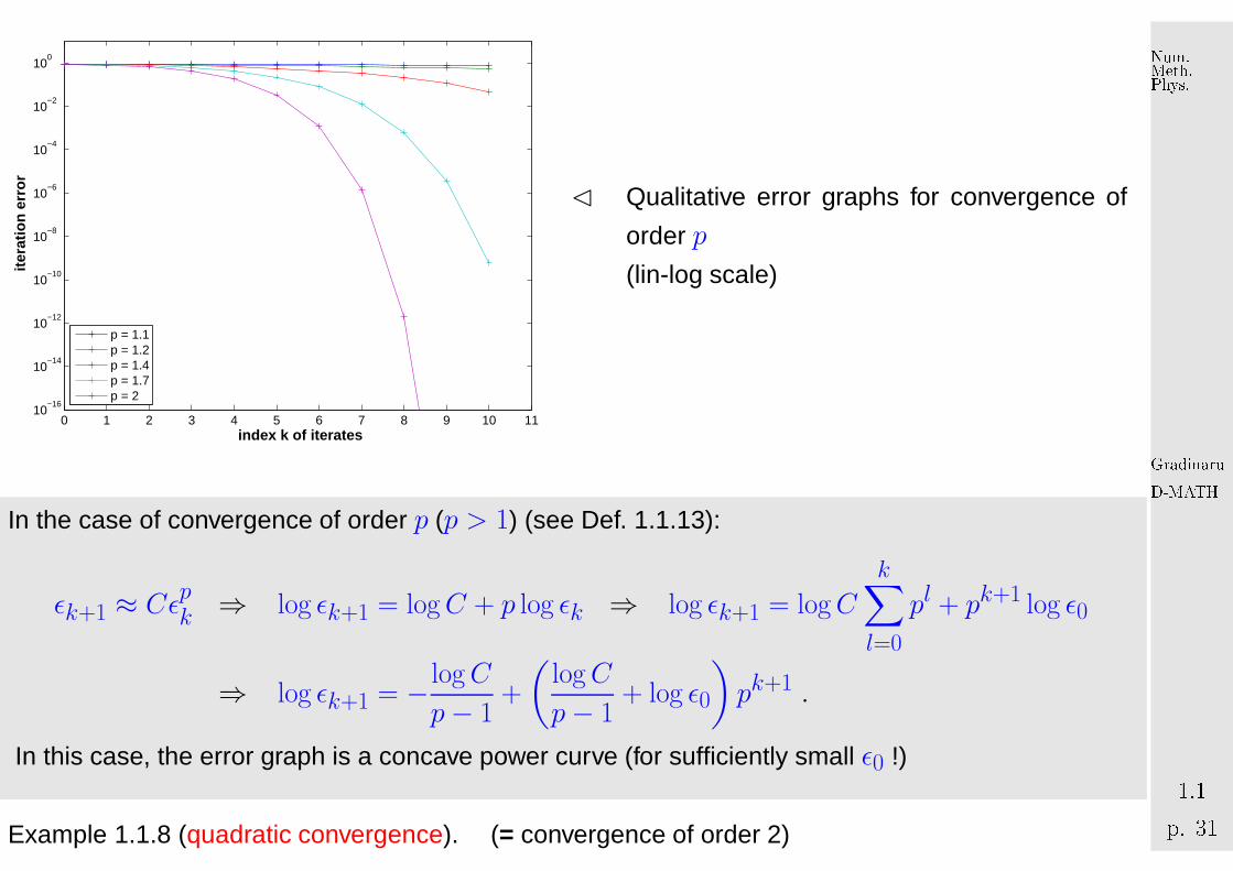
0 1 2 3 4 5 6 7 8 9 10 1110

−16

10−14

10−12

10−10

10−8

10−6

10−4

10−2

100

index k of iterates

iter

atio

n er

ror

p = 1.1p = 1.2p = 1.4p = 1.7p = 2

� Qualitative error graphs for convergence of

order p

(lin-log scale)

In the case of convergence of order p (p > 1) (see Def. 1.1.13):

ǫk+1 ≈ Cǫpk ⇒ log ǫk+1 = logC + p log ǫk ⇒ log ǫk+1 = logC

k∑

l=0

pl + pk+1 log ǫ0

⇒ log ǫk+1 = − logC

p− 1+

(logC

p− 1+ log ǫ0

)pk+1 .

In this case, the error graph is a concave power curve (for sufficiently small ǫ0 !)

Example 1.1.8 (quadratic convergence). (= convergence of order 2)


Num.Meth.Phys.

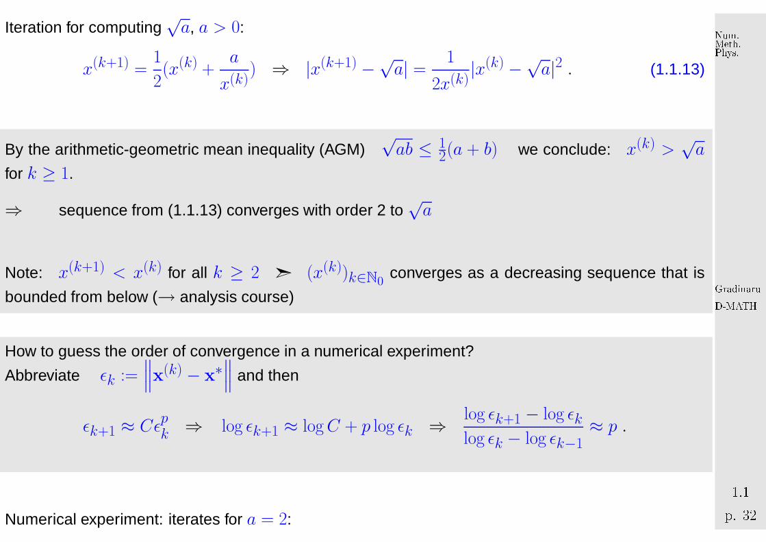
Iteration for computing√a, a > 0:

x(k+1) =1

2(x(k) +

a

x(k)) ⇒ |x(k+1) −√a| = 1

2x(k)|x(k) −√a|2 . (1.1.13)

By the arithmetic-geometric mean inequality (AGM)√ab ≤ 1

2(a + b) we conclude: x(k) >√a

for k ≥ 1.

⇒ sequence from (1.1.13) converges with order 2 to√a

Note: x(k+1) < x(k) for all k ≥ 2 ➣ (x(k))k∈N0converges as a decreasing sequence that is

bounded from below (→ analysis course)

How to guess the order of convergence in a numerical experiment?

Abbreviate ǫk :=∥∥∥x(k) − x∗

∥∥∥ and then

ǫk+1 ≈ Cǫpk ⇒ log ǫk+1 ≈ logC + p log ǫk ⇒

log ǫk+1 − log ǫklog ǫk − log ǫk−1

≈ p .

Numerical experiment: iterates for a = 2:


Num.Meth.Phys.

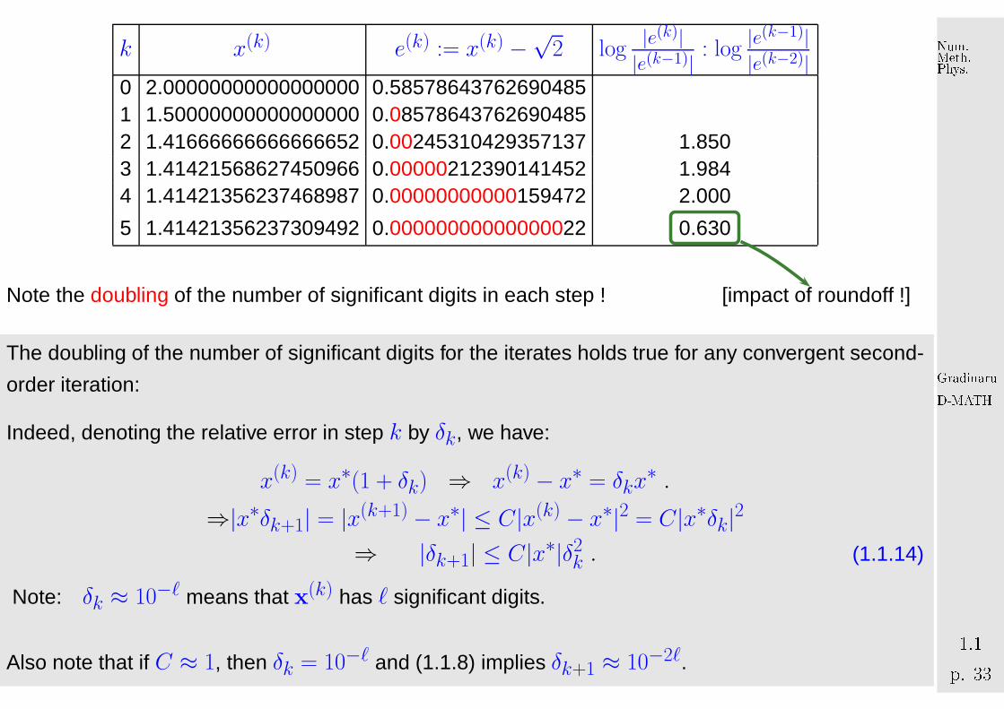
k x(k) e(k) := x(k) −√

2 log|e(k)||e(k−1)| : log

|e(k−1)||e(k−2)|

0 2.00000000000000000 0.585786437626904851 1.50000000000000000 0.085786437626904852 1.41666666666666652 0.00245310429357137 1.8503 1.41421568627450966 0.00000212390141452 1.9844 1.41421356237468987 0.00000000000159472 2.000

5 1.41421356237309492 0.00000000000000022 0.630

Note the doubling of the number of significant digits in each step ! [impact of roundoff !]

The doubling of the number of significant digits for the iterates holds true for any convergent second-

order iteration:

Indeed, denoting the relative error in step k by δk, we have:

x(k) = x∗(1 + δk) ⇒ x(k) − x∗ = δkx∗ .

⇒|x∗δk+1| = |x(k+1) − x∗| ≤ C|x(k) − x∗|2 = C|x∗δk|2⇒ |δk+1| ≤ C|x∗|δ2k . (1.1.14)

Note: δk ≈ 10−ℓ means that x(k) has ℓ significant digits.

Also note that if C ≈ 1, then δk = 10−ℓ and (1.1.8) implies δk+1 ≈ 10−2ℓ.


Num.Meth.Phys.

3

1.1.2 Termination criteria

Usually (even without roundoff errors) the iteration will never arrive at an/the exact solution x∗ after

finitely many steps. Thus, we can only hope to compute an approximate solution by accepting x(K)

as result for some K ∈ N0. Termination criteria (ger.: Abbruchbedingungen) are used to determine

a suitable value for K.

For the sake of efficiency: � stop iteration when iteration error is just “small enough”

“small enough” depends on concrete setting:

Usual goal:∥∥∥x(K) − x∗

∥∥∥ ≤ τ , τ =̂ prescribed tolerance.

Ideal: K = argmin{k ∈ N0:∥∥∥x(k) − x∗

∥∥∥ < τ} . (1.1.15)


Num.Meth.Phys.

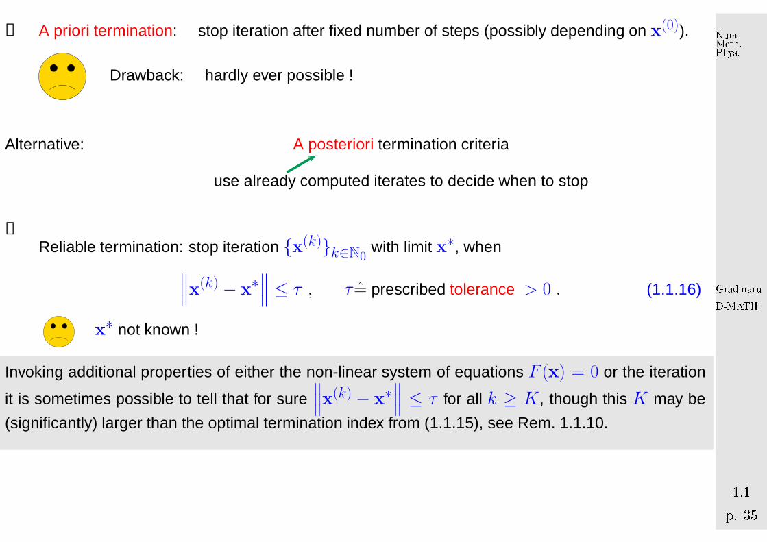
➀ A priori termination: stop iteration after fixed number of steps (possibly depending on x(0)).

Drawback: hardly ever possible !

Alternative: A posteriori termination criteria

use already computed iterates to decide when to stop

➁Reliable termination: stop iteration {x(k)}k∈N0

with limit x∗, when∥∥∥x(k) − x∗

∥∥∥ ≤ τ , τ =̂ prescribed tolerance > 0 . (1.1.16)

x∗ not known !

Invoking additional properties of either the non-linear system of equations F (x) = 0 or the iteration

it is sometimes possible to tell that for sure∥∥∥x(k) − x∗

∥∥∥ ≤ τ for all k ≥ K, though this K may be

(significantly) larger than the optimal termination index from (1.1.15), see Rem. 1.1.10.


Num.Meth.Phys.

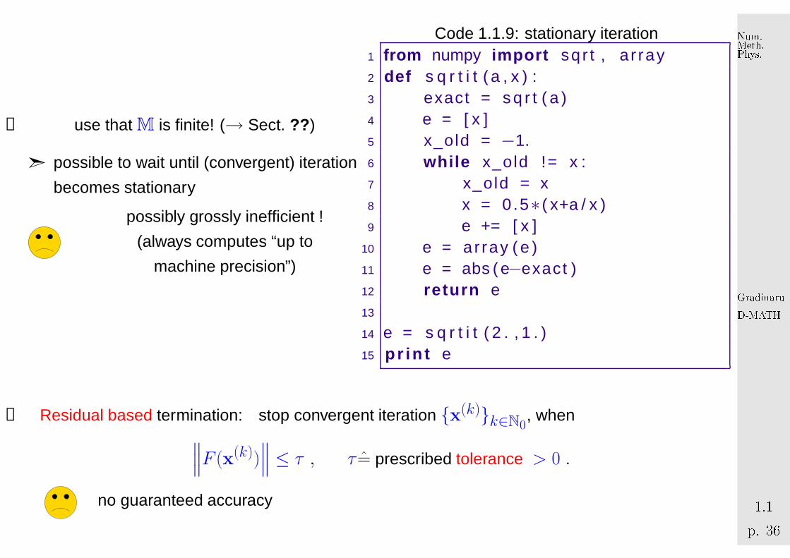
➂ use that M is finite! (→ Sect. ?? )

➣ possible to wait until (convergent) iteration

becomes stationary

possibly grossly inefficient !

(always computes “up to

machine precision”)

Code 1.1.9: stationary iteration1 from numpy impo r t sqr t , a r ray2 def s q r t i t ( a , x ) :3 exact = s q r t ( a )4 e = [ x ]5 x_old = −1.6 w h il e x_old != x :7 x_old = x8 x = 0.5∗ ( x+a / x )9 e += [ x ]

10 e = ar ray ( e )11 e = abs ( e−exact )12 r et u r n e13

14 e = s q r t i t ( 2 . , 1 . )15 p r i n t e

➃ Residual based termination: stop convergent iteration {x(k)}k∈N0, when

∥∥∥F (x(k))∥∥∥ ≤ τ , τ =̂ prescribed tolerance > 0 .

no guaranteed accuracy


Num.Meth.Phys.

F (x)

x

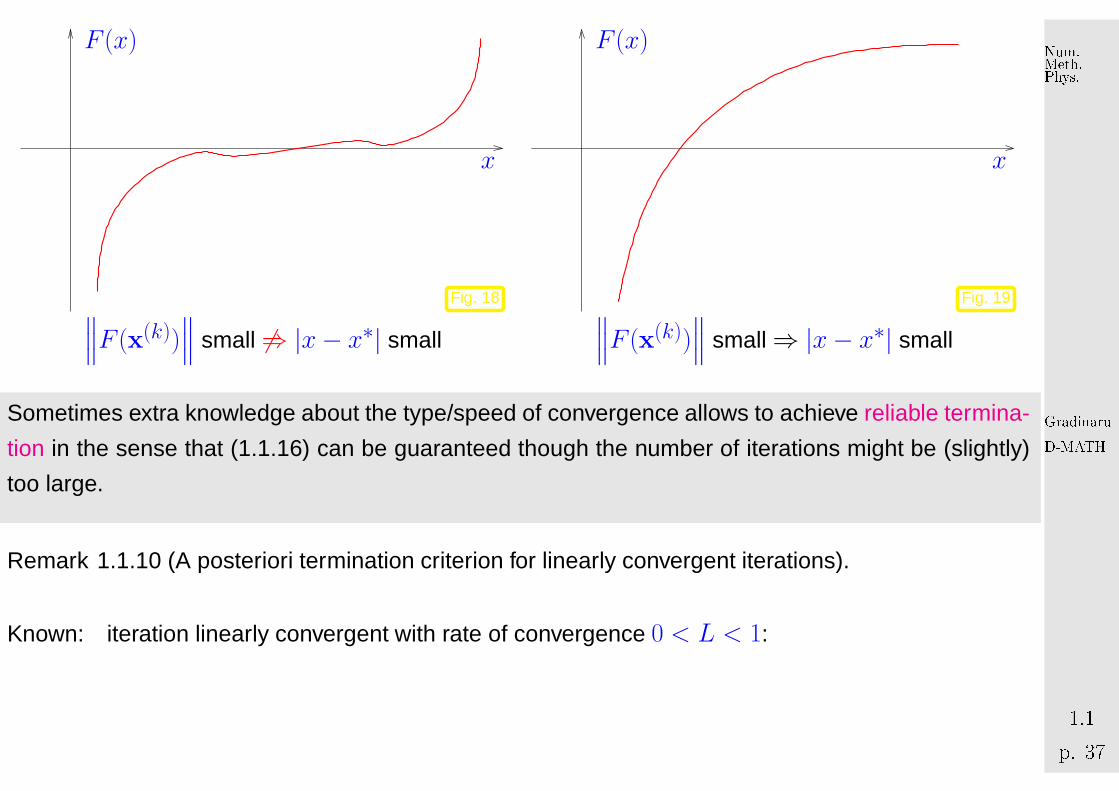
Fig. 18∥∥∥F (x(k))∥∥∥ small 6⇒ |x− x∗| small

F (x)

x

Fig. 19∥∥∥F (x(k))∥∥∥ small⇒ |x− x∗| small

Sometimes extra knowledge about the type/speed of convergence allows to achieve reliable termina-

tion in the sense that (1.1.16) can be guaranteed though the number of iterations might be (slightly)

too large.

Remark 1.1.10 (A posteriori termination criterion for linearly convergent iterations).

Known: iteration linearly convergent with rate of convergence 0 < L < 1:


Num.Meth.Phys.

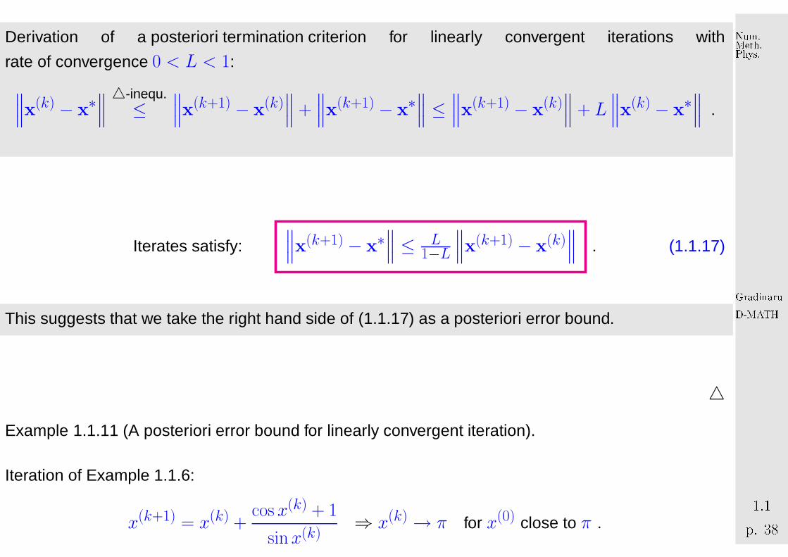
Derivation of a posteriori termination criterion for linearly convergent iterations with

rate of convergence 0 < L < 1:

∥∥∥x(k) − x∗∥∥∥△-inequ.≤

∥∥∥x(k+1) − x(k)∥∥∥ +

∥∥∥x(k+1) − x∗∥∥∥ ≤

∥∥∥x(k+1) − x(k)∥∥∥ + L

∥∥∥x(k) − x∗∥∥∥ .

Iterates satisfy:∥∥∥x(k+1) − x∗

∥∥∥ ≤ L1−L

∥∥∥x(k+1) − x(k)∥∥∥ . (1.1.17)

This suggests that we take the right hand side of (1.1.17) as a posteriori error bound.

△

Example 1.1.11 (A posteriori error bound for linearly convergent iteration).

Iteration of Example 1.1.6:

x(k+1) = x(k) +cos x(k) + 1

sinx(k)⇒ x(k) → π for x(0) close to π .


Num.Meth.Phys.

Observed rate of convergence: L = 1/2

Error and error bound for x(0) = 0.4:

k |x(k) − π| L1−L|x(k) − x(k−1)| slack of bound

1 2.191562221997101 4.933154875586894 2.7415926535897932 0.247139097781070 1.944423124216031 1.6972840264349613 0.122936737876834 0.124202359904236 0.0012656220274014 0.061390835206217 0.061545902670618 0.0001550674644015 0.030685773472263 0.030705061733954 0.0000192882616916 0.015341682696235 0.015344090776028 0.0000024080797927 0.007670690889185 0.007670991807050 0.0000003009178648 0.003835326638666 0.003835364250520 0.0000000376118549 0.001917660968637 0.001917665670029 0.00000000470139210 0.000958830190489 0.000958830778147 0.00000000058765811 0.000479415058549 0.000479415131941 0.00000000007339212 0.000239707524646 0.000239707533903 0.00000000000925713 0.000119853761949 0.000119853762696 0.00000000000074714 0.000059926881308 0.000059926880641 0.00000000000066715 0.000029963440745 0.000029963440563 0.000000000000181

Hence: the a posteriori error bound is highly accurate in this case!3


Num.Meth.Phys.

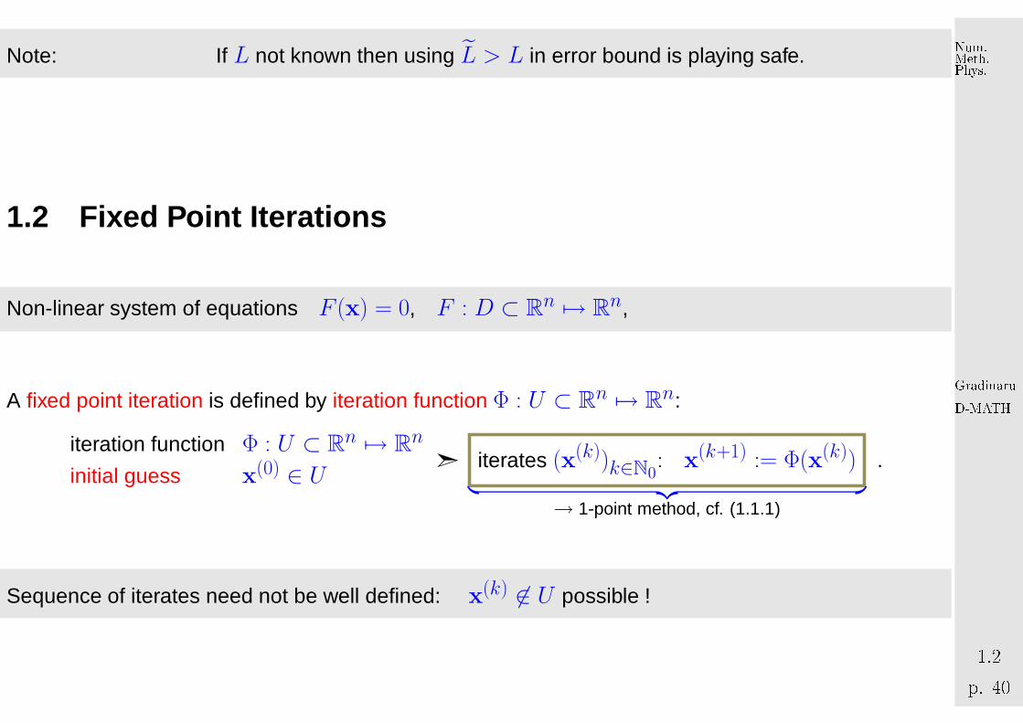
Note: If L not known then using L̃ > L in error bound is playing safe.

1.2 Fixed Point Iterations

Non-linear system of equations F (x) = 0, F : D ⊂ Rn 7→ R

n,

A fixed point iteration is defined by iteration function Φ : U ⊂ Rn 7→ Rn:

iteration function Φ : U ⊂ Rn 7→ Rn

initial guess x(0) ∈ U ➣ iterates (x(k))k∈N0: x(k+1) := Φ(x(k))

︸︷︷︸→ 1-point method, cf. (1.1.1)

.

Sequence of iterates need not be well defined: x(k) 6∈ U possible !


Num.Meth.Phys.

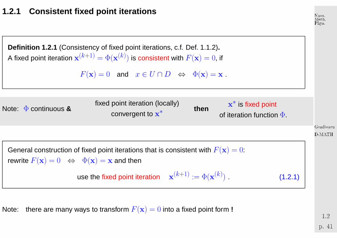
1.2.1 Consistent fixed po int iterations

Defin ition 1.2.1 (Consistency of fixed point iterations, c.f. Def. 1.1.2).

A fixed point iteration x(k+1) = Φ(x(k)) is consistent with F (x) = 0, if

F (x) = 0 and x ∈ U ∩D ⇔ Φ(x) = x .

Note: Φ continuous &fixed point iteration (locally)

convergent to x∗then

x∗ is fixed point

of iteration function Φ.

General construction of fixed point iterations that is consistent with F (x) = 0:

rewrite F (x) = 0 ⇔ Φ(x) = x and then

use the fixed point iteration x(k+1) := Φ(x(k)) . (1.2.1)

Note: there are many ways to transform F (x) = 0 into a fixed point form !


Num.Meth.Phys.

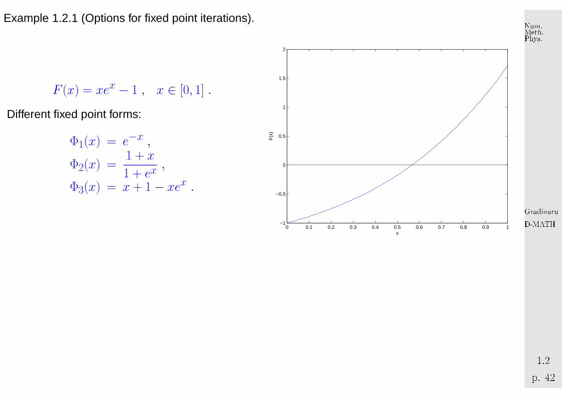
Example 1.2.1 (Options for fixed point iterations).

F (x) = xex − 1 , x ∈ [0, 1] .

Different fixed point forms:

Φ1(x) = e−x ,

Φ2(x) =1 + x

1 + ex,

Φ3(x) = x + 1− xex .

0 0.1 0.2 0.3 0.4 0.5 0.6 0.7 0.8 0.9 1−1

−0.5

0

0.5

1

1.5

2

x

F(x

)


Num.Meth.Phys.

0 0.1 0.2 0.3 0.4 0.5 0.6 0.7 0.8 0.9 10

0.1

0.2

0.3

0.4

0.5

0.6

0.7

0.8

0.9

1

x

Φ

function Φ1

0 0.1 0.2 0.3 0.4 0.5 0.6 0.7 0.8 0.9 10

0.1

0.2

0.3

0.4

0.5

0.6

0.7

0.8

0.9

1

Φ

x

function Φ2

0 0.1 0.2 0.3 0.4 0.5 0.6 0.7 0.8 0.9 10

0.1

0.2

0.3

0.4

0.5

0.6

0.7

0.8

0.9

1

x

Φ

function Φ3

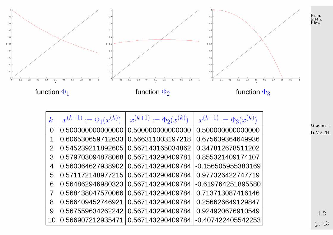
k x(k+1) := Φ1(x(k)) x(k+1) := Φ2(x

(k)) x(k+1) := Φ3(x(k))

0 0.500000000000000 0.500000000000000 0.5000000000000001 0.606530659712633 0.566311003197218 0.6756393646499362 0.545239211892605 0.567143165034862 0.3478126785112023 0.579703094878068 0.567143290409781 0.8553214091741074 0.560064627938902 0.567143290409784 -0.1565059553831695 0.571172148977215 0.567143290409784 0.9773264227477196 0.564862946980323 0.567143290409784 -0.6197642518955807 0.568438047570066 0.567143290409784 0.7137130874161468 0.566409452746921 0.567143290409784 0.2566266491298479 0.567559634262242 0.567143290409784 0.92492067691054910 0.566907212935471 0.567143290409784 -0.407422405542253


Num.Meth.Phys.

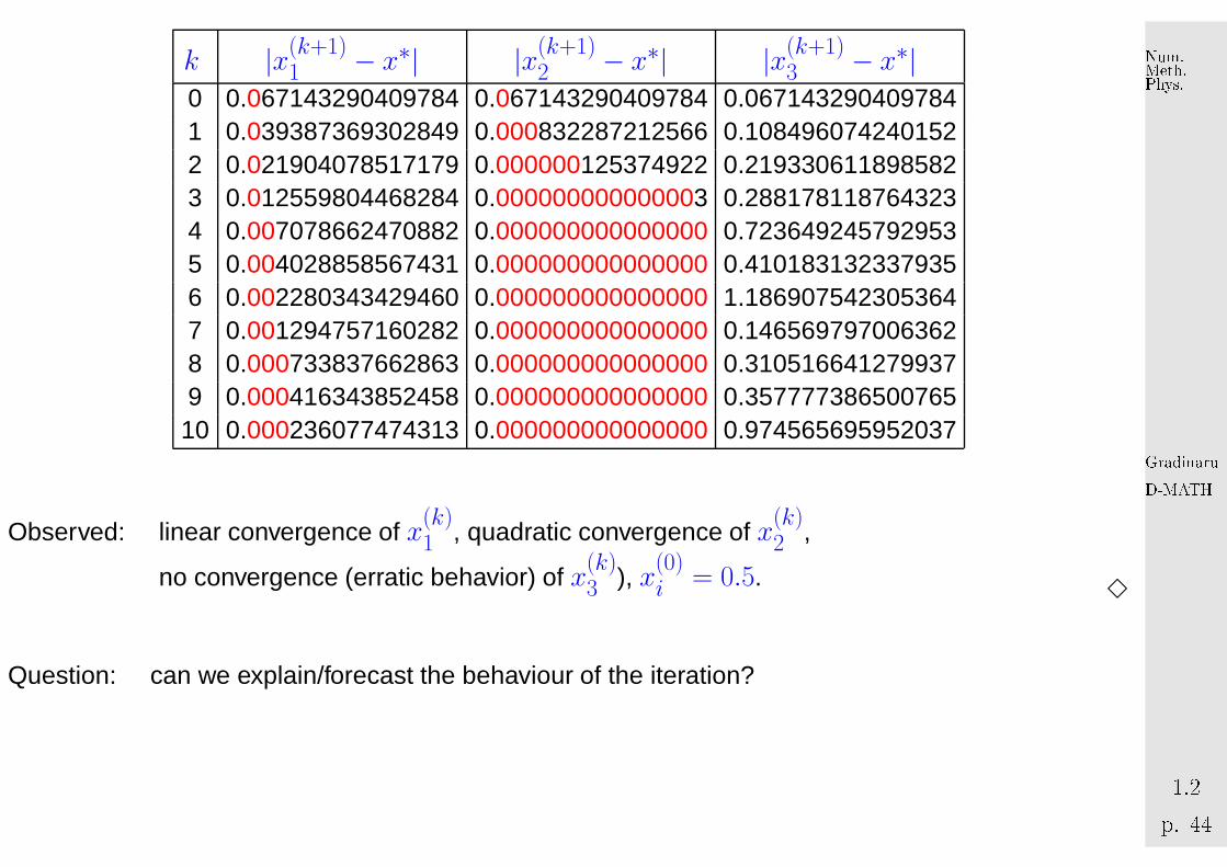
k |x(k+1)1 − x∗| |x(k+1)

2 − x∗| |x(k+1)3 − x∗|

0 0.067143290409784 0.067143290409784 0.0671432904097841 0.039387369302849 0.000832287212566 0.1084960742401522 0.021904078517179 0.000000125374922 0.2193306118985823 0.012559804468284 0.000000000000003 0.2881781187643234 0.007078662470882 0.000000000000000 0.7236492457929535 0.004028858567431 0.000000000000000 0.4101831323379356 0.002280343429460 0.000000000000000 1.1869075423053647 0.001294757160282 0.000000000000000 0.1465697970063628 0.000733837662863 0.000000000000000 0.3105166412799379 0.000416343852458 0.000000000000000 0.35777738650076510 0.000236077474313 0.000000000000000 0.974565695952037

Observed: linear convergence of x(k)1 , quadratic convergence of x

(k)2 ,

no convergence (erratic behavior) of x(k)3 ), x

(0)i = 0.5.

3

Question: can we explain/forecast the behaviour of the iteration?


Num.Meth.Phys.

1.2.2 Convergence of fixed po int iterations

In this section we will try to find easily verifiable conditions that ensure convergence (of a certain order)

of fixed point iterations. It will turn out that these conditions are surprisingly simple and general.

Defin ition 1.2.2 (Contractive mapping).

Φ : U ⊂ Rn 7→ R

n is contractive (w.r.t. norm ‖·‖ on Rn), if

∃L < 1: ‖Φ(x)− Φ(y)‖ ≤ L ‖x− y‖ ∀x,y ∈ U . (1.2.2)

A simple consideration: if Φ(x∗) = x∗ (fixed point), then a fixed point iteration induced by a

contractive mapping Φ satisfies

∥∥∥x(k+1) − x∗∥∥∥ =

∥∥∥Φ(x(k))− Φ(x∗)∥∥∥

(1.2.3)≤ L

∥∥∥x(k) − x∗∥∥∥ ,

that is, the iteration converges (at least) linearly (→ Def. 1.1.4).

Remark 1.2.2 (Banach’s fixed point theorem). → [?, Satz 6.5.2]

A key theorem in calculus (also functional analysis):


Num.Meth.Phys.

'

&

$

%

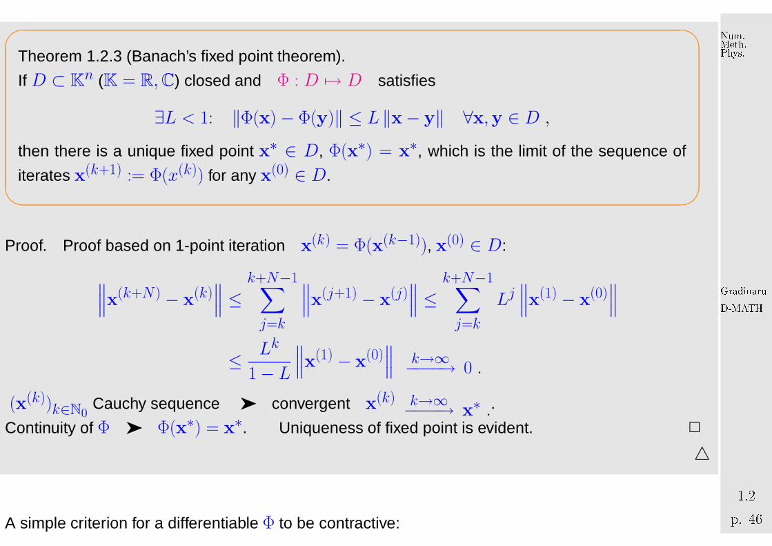
Theorem 1.2.3 (Banach’s fixed point theorem).

If D ⊂ Kn (K = R,C) closed and Φ : D 7→ D satisfies

∃L < 1: ‖Φ(x)− Φ(y)‖ ≤ L ‖x− y‖ ∀x,y ∈ D ,

then there is a unique fixed point x∗ ∈ D, Φ(x∗) = x∗, which is the limit of the sequence of

iterates x(k+1) := Φ(x(k)) for any x(0) ∈ D.

Proof. Proof based on 1-point iteration x(k) = Φ(x(k−1)), x(0) ∈ D:

∥∥∥x(k+N) − x(k)∥∥∥ ≤

k+N−1∑

j=k

∥∥∥x(j+1) − x(j)∥∥∥ ≤

k+N−1∑

j=k

Lj∥∥∥x(1) − x(0)

∥∥∥

≤ Lk

1− L∥∥∥x(1) − x(0)

∥∥∥ k→∞−−−−→ 0 .

(x(k))k∈N0Cauchy sequence ➤ convergent x(k) k→∞−−−−→ x∗ ..

Continuity of Φ ➤ Φ(x∗) = x∗. Uniqueness of fixed point is evident. 2

△

A simple criterion for a differentiable Φ to be contractive:


Num.Meth.Phys.

'

&

$

%

Lemma 1.2.4 (Sufficient condition for local linear convergence of fixed point iteration).

If Φ : U ⊂ Rn 7→ R

n, Φ(x∗) = x∗,Φ differentiable in x∗, and ‖DΦ(x∗)‖ < 1, then the fixed

point iteration (1.2.1) converges locally and at least linearly.

matrix norm, Def. 1.1.12 !

✎ notation: DΦ(x) =̂ Jacobian (ger.: Jacobi-Matrix) of Φ at x ∈ D

Example 1.2.3 (Fixed point iteration in 1D).

1D setting (n = 1): Φ : R 7→ R continuously differentiable, Φ(x∗) = x∗

fixed point iteration: x(k+1) = Φ(x(k))

“Visualization” of the statement of Lemma 1.2.4: The iteration converges locally, if Φ is flat in a

neighborhood of x∗, it will diverge, if Φ is steep there.


Num.Meth.Phys.

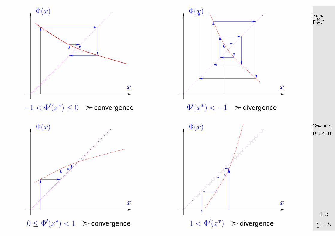
x

Φ(x)

−1 < Φ′(x∗) ≤ 0 ➣ convergence

x

Φ(x)

Φ′(x∗) < −1 ➣ divergence

x

Φ(x)

0 ≤ Φ′(x∗) < 1 ➣ convergence

x

Φ(x)

1 < Φ′(x∗) ➣ divergence


Num.Meth.Phys.

3

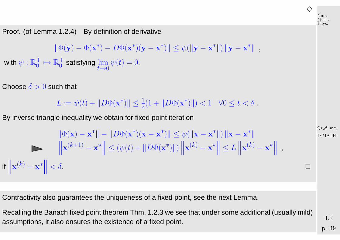
Proof. (of Lemma 1.2.4) By definition of derivative

‖Φ(y)− Φ(x∗)−DΦ(x∗)(y − x∗)‖ ≤ ψ(‖y − x∗‖) ‖y − x∗‖ ,with ψ : R

+0 7→ R

+0 satisfying lim

t→0ψ(t) = 0.

Choose δ > 0 such that

L := ψ(t) + ‖DΦ(x∗)‖ ≤ 12(1 + ‖DΦ(x∗)‖) < 1 ∀0 ≤ t < δ .

By inverse triangle inequality we obtain for fixed point iteration

‖Φ(x)− x∗‖ − ‖DΦ(x∗)(x− x∗)‖ ≤ ψ(‖x− x∗‖) ‖x− x∗‖∥∥∥x(k+1) − x∗∥∥∥ ≤ (ψ(t) + ‖DΦ(x∗)‖)

∥∥∥x(k) − x∗∥∥∥ ≤ L

∥∥∥x(k) − x∗∥∥∥ ,

if∥∥∥x(k) − x∗

∥∥∥ < δ. 2

Contractivity also guarantees the uniqueness of a fixed point, see the next Lemma.

Recalling the Banach fixed point theorem Thm. 1.2.3 we see that under some additional (usually mild)assumptions, it also ensures the existence of a fixed point.


Num.Meth.Phys.

'

&

$

%

Lemma 1.2.5 (Sufficient condition for local linear convergence of fixed point iteration (II)).

Let U be convex and Φ : U ⊂ Rn 7→ R

n continuously differentiable with L := supx∈U‖DΦ(x)‖ <

1. If Φ(x∗) = x∗ for some interior point x∗ ∈ U , then the fixed point iteration x(k+1) = Φ(x(k))

converges to x∗ locally at least linearly.

Recall: U ⊂ Rn convex :⇔ (tx + (1− t)y) ∈ U for all x,y ∈ U , 0 ≤ t ≤ 1

Proof. (of Lemma 1.2.5) By the mean value theorem

Φ(x)− Φ(y) =

∫ 1

0DΦ(x + τ (y − x))(y − x) dτ ∀x,y ∈ dom(Φ) .

‖Φ(x)− Φ(y)‖ ≤ L ‖y − x‖ .There is δ > 0: B := {x: ‖x− x∗‖ ≤ δ} ⊂ dom(Φ). Φ is contractive on B with unique fixed point

x∗.

Remark 1.2.4.

If 0 < ‖DΦ(x∗)‖ < 1, x(k) ≈ x∗ then the asymptotic rate of linear convergence is L = ‖DΦ(x∗)‖

△


Num.Meth.Phys.

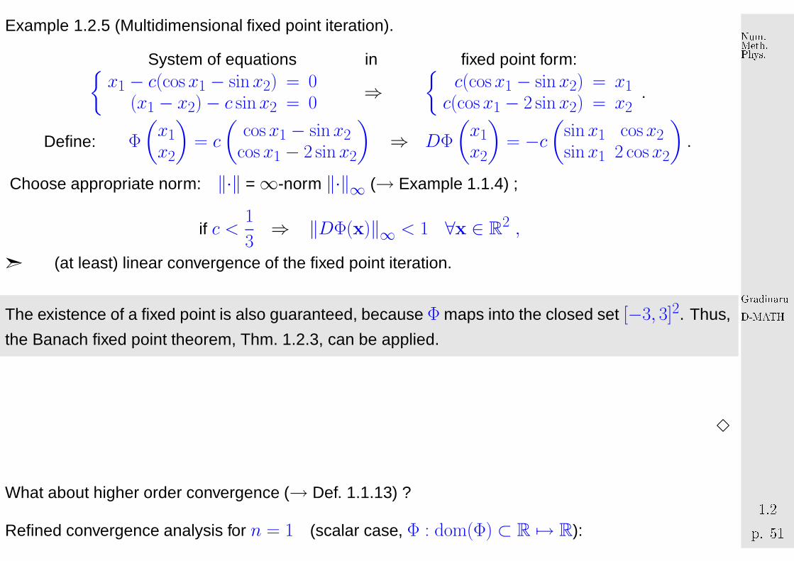
Example 1.2.5 (Multidimensional fixed point iteration).

System of equations in fixed point form:{x1 − c(cosx1 − sinx2) = 0

(x1 − x2)− c sinx2 = 0⇒

{c(cosx1 − sin x2) = x1c(cosx1 − 2 sin x2) = x2

.

Define: Φ

(x1x2

)= c

(cosx1 − sinx2

cos x1 − 2 sin x2

)⇒ DΦ

(x1x2

)= −c

(sinx1 cosx2sinx1 2 cosx2

).

Choose appropriate norm: ‖·‖ =∞-norm ‖·‖∞ (→ Example 1.1.4) ;

if c <1

3⇒ ‖DΦ(x)‖∞ < 1 ∀x ∈ R

2 ,

➣ (at least) linear convergence of the fixed point iteration.

The existence of a fixed point is also guaranteed, because Φ maps into the closed set [−3, 3]2. Thus,

the Banach fixed point theorem, Thm. 1.2.3, can be applied.

3

What about higher order convergence (→ Def. 1.1.13) ?

Refined convergence analysis for n = 1 (scalar case, Φ : dom(Φ) ⊂ R 7→ R):


Num.Meth.Phys.

'

&

$

%

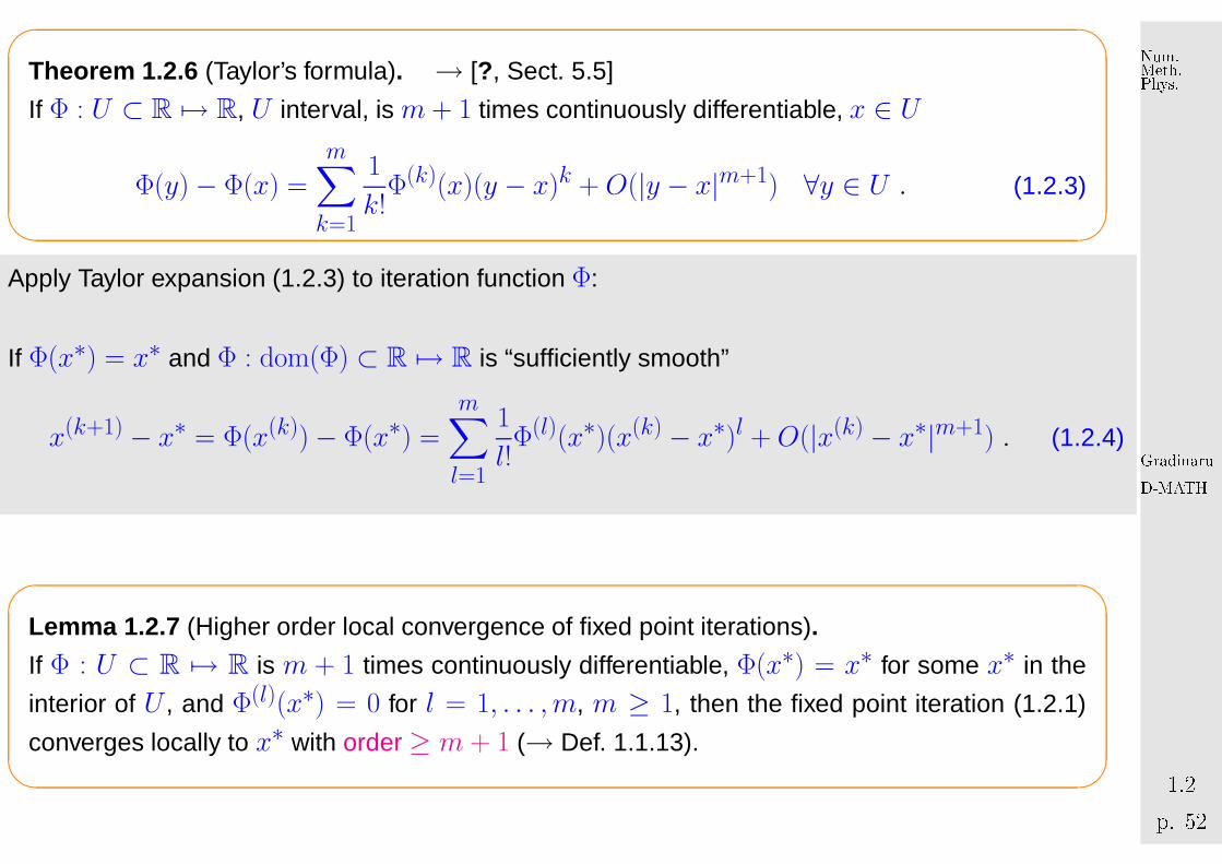
Theorem 1.2.6 (Taylor’s formula). → [?, Sect. 5.5]

If Φ : U ⊂ R 7→ R, U interval, is m + 1 times continuously differentiable, x ∈ U

Φ(y)− Φ(x) =m∑

k=1

1

k!Φ(k)(x)(y − x)k +O(|y − x|m+1) ∀y ∈ U . (1.2.3)

Apply Taylor expansion (1.2.3) to iteration function Φ:

If Φ(x∗) = x∗ and Φ : dom(Φ) ⊂ R 7→ R is “sufficiently smooth”

x(k+1) − x∗ = Φ(x(k))− Φ(x∗) =

m∑

l=1

1

l!Φ(l)(x∗)(x(k) − x∗)l +O(|x(k) − x∗|m+1) . (1.2.4)

'

&

$

%

Lemma 1.2.7 (Higher order local convergence of fixed point iterations).

If Φ : U ⊂ R 7→ R is m + 1 times continuously differentiable, Φ(x∗) = x∗ for some x∗ in the

interior of U , and Φ(l)(x∗) = 0 for l = 1, . . . ,m, m ≥ 1, then the fixed point iteration (1.2.1)

converges locally to x∗ with order ≥ m + 1 (→ Def. 1.1.13).


Num.Meth.Phys.

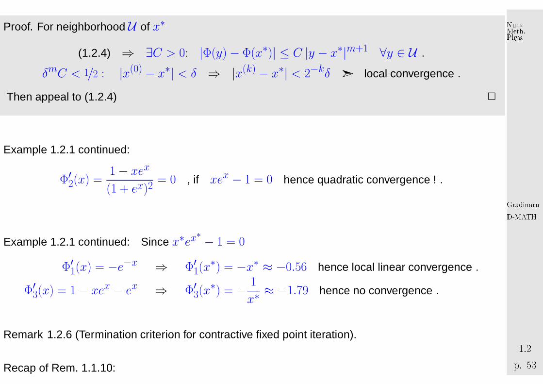
Proof. For neighborhood U of x∗

(1.2.4) ⇒ ∃C > 0: |Φ(y)− Φ(x∗)| ≤ C |y − x∗|m+1 ∀y ∈ U .δmC < 1/2 : |x(0) − x∗| < δ ⇒ |x(k) − x∗| < 2−kδ ➣ local convergence .

Then appeal to (1.2.4) 2

Example 1.2.1 continued:

Φ′2(x) =1− xex(1 + ex)2

= 0 , if xex − 1 = 0 hence quadratic convergence ! .

Example 1.2.1 continued: Since x∗ex∗ − 1 = 0

Φ′1(x) = −e−x ⇒ Φ′1(x∗) = −x∗ ≈ −0.56 hence local linear convergence .

Φ′3(x) = 1− xex − ex ⇒ Φ′3(x∗) = − 1

x∗≈ −1.79 hence no convergence .

Remark 1.2.6 (Termination criterion for contractive fixed point iteration).

Recap of Rem. 1.1.10:


Num.Meth.Phys.

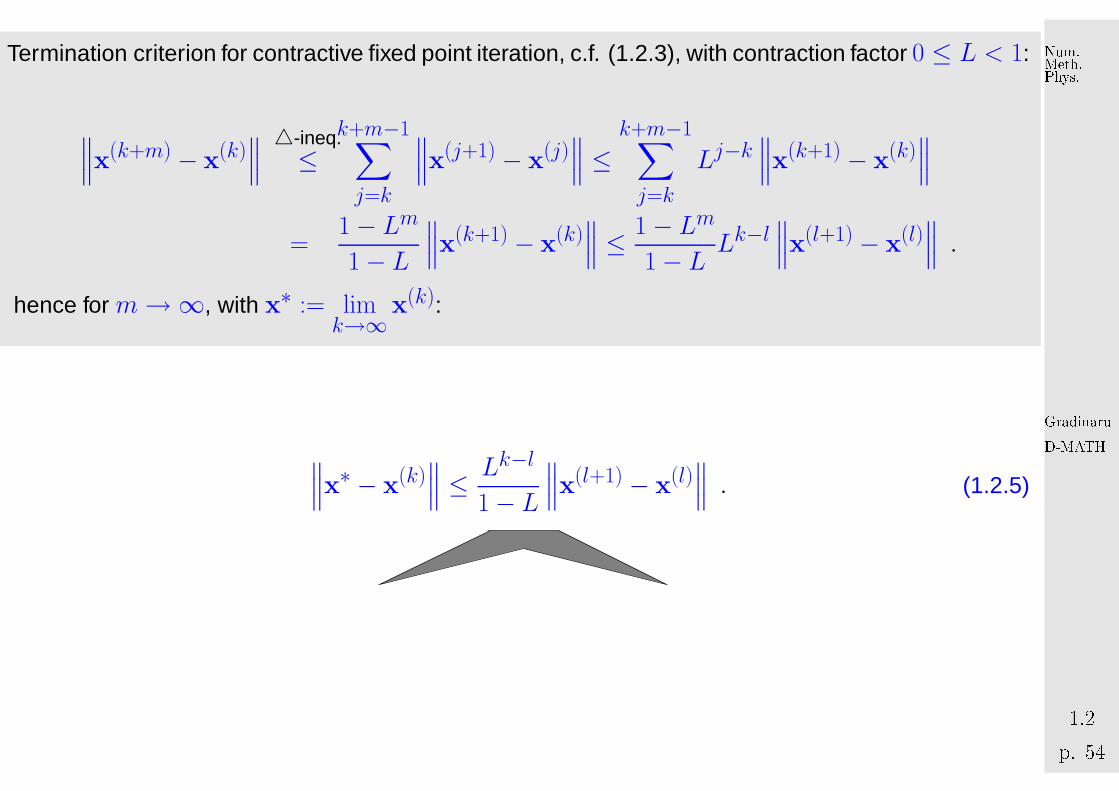
Termination criterion for contractive fixed point iteration, c.f. (1.2.3), with contraction factor 0 ≤ L < 1:

∥∥∥x(k+m) − x(k)∥∥∥△-ineq.≤

k+m−1∑

j=k

∥∥∥x(j+1) − x(j)∥∥∥ ≤

k+m−1∑

j=k

Lj−k∥∥∥x(k+1) − x(k)

∥∥∥

=1− Lm1− L

∥∥∥x(k+1) − x(k)∥∥∥ ≤ 1− Lm

1− L Lk−l∥∥∥x(l+1) − x(l)

∥∥∥ .

hence for m→∞, with x∗ := limk→∞

x(k):

∥∥∥x∗ − x(k)∥∥∥ ≤ Lk−l

1− L∥∥∥x(l+1) − x(l)

∥∥∥ . (1.2.5)


Num.Meth.Phys.

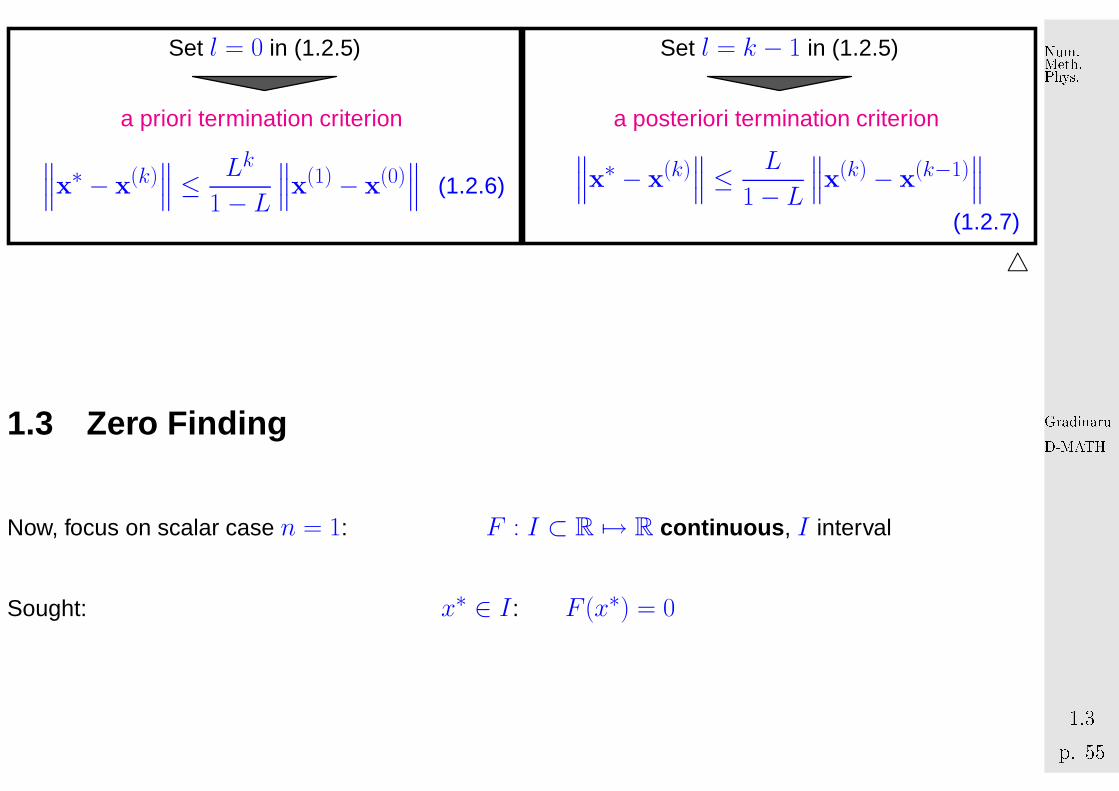
Set l = 0 in (1.2.5)

a priori termination criterion

∥∥∥x∗ − x(k)∥∥∥ ≤ Lk

1− L∥∥∥x(1) − x(0)

∥∥∥ (1.2.6)

Set l = k − 1 in (1.2.5)

a posteriori termination criterion∥∥∥x∗ − x(k)

∥∥∥ ≤ L

1− L∥∥∥x(k) − x(k−1)

∥∥∥(1.2.7)

△

1.3 Zero Find ing

Now, focus on scalar case n = 1: F : I ⊂ R 7→ R continuou s, I interval

Sought: x∗ ∈ I : F (x∗) = 0


Num.Meth.Phys.

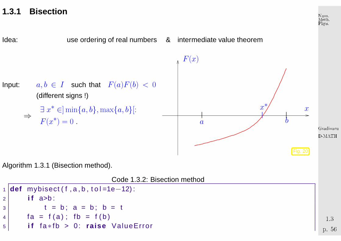
1.3.1 Bisection

Idea: use ordering of real numbers & intermediate value theorem

Input: a, b ∈ I such that F (a)F (b) < 0

(different signs !)

⇒ ∃ x∗ ∈] min{a, b},max{a, b}[:F (x∗) = 0 .

xx∗

F (x)

a b

Fig. 20

Algorithm 1.3.1 (Bisection method).

Code 1.3.2: Bisection method1 def mybisect ( f , a , b , t o l =1e−12) :2 i f a>b :3 t = b ; a = b ; b = t4 fa = f ( a ) ; fb = f ( b )5 i f fa∗ fb > 0 : r a i se ValueError


Num.Meth.Phys.

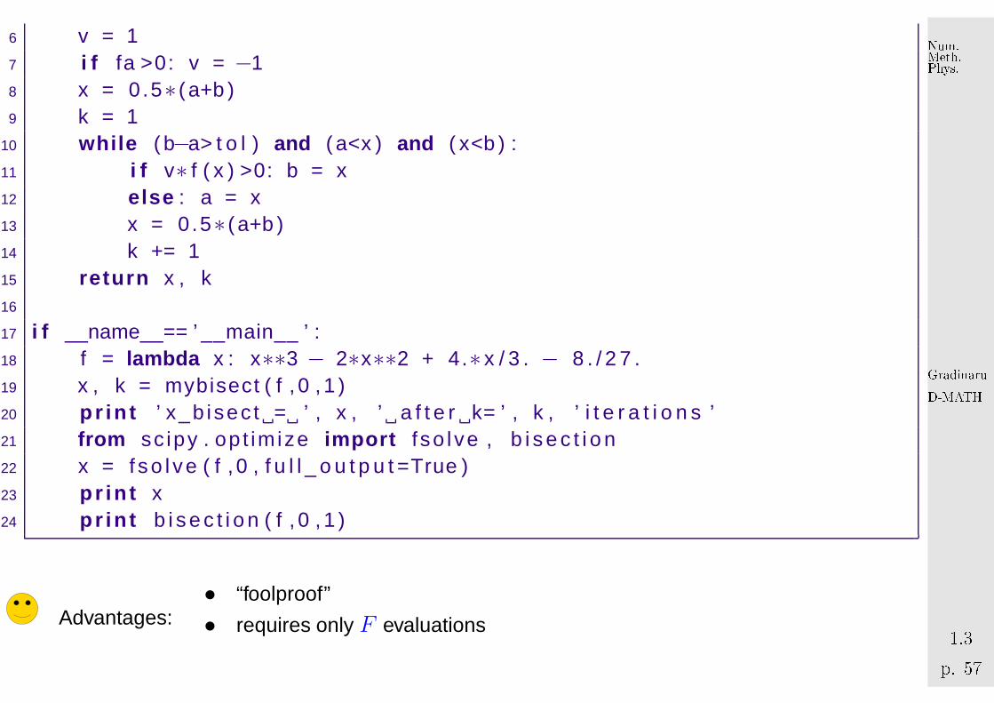
6 v = 17 i f fa >0: v = −18 x = 0.5∗ ( a+b )9 k = 1

10 w h il e ( b−a> t o l ) and ( a<x ) and ( x<b ) :11 i f v∗ f ( x ) >0: b = x12 el se : a = x13 x = 0.5∗ ( a+b )14 k += 115 r et u r n x , k16

17 i f __name__== ’ __main__ ’ :18 f = lambda x : x∗∗3 − 2∗x∗∗2 + 4.∗ x / 3 . − 8 . / 2 7 .19 x , k = mybisect ( f , 0 , 1 )20 p r i n t ’ x_b isec t = ’ , x , ’ a f t e r k= ’ , k , ’ i t e r a t i o n s ’21 from sc ipy . op t im ize impo r t f so lve , b i s e c t i o n22 x = f so l ve ( f , 0 , f u l l _ o u t p u t =True )23 p r i n t x24 p r i n t b i s e c t i o n ( f , 0 , 1 )

Advantages:• “foolproof”

• requires only F evaluations


Num.Meth.Phys.

Drawbacks:

Merely linear convergence: |x(k) − x∗| ≤ 2−k|b− a|log2

(|b− a|tol

)steps necessary

1.3.2 Model function method s

=̂ class of iterative methods for finding zeroes of F :

Idea: Given: approximate zeroes x(k), x(k−1), . . . , x(k−m)

➊ replace F with model function F̃

(using function values/derivative values in x(k), x(k−1), . . . , x(k−m))

➋ x(k+1) := zero of F̃

(has to be readily available↔ analytic formula)

Distinguish (see (1.1.1)):

one-point methods : x(k+1) = ΦF (x(k)), k ∈ N (e.g., fixed point iteration→ Sect. 1.2)

multi-point methods : x(k+1) = ΦF (x(k), x(k−1), . . . , x(k−m)), k ∈ N, m = 2, 3, . . ..


Num.Meth.Phys.

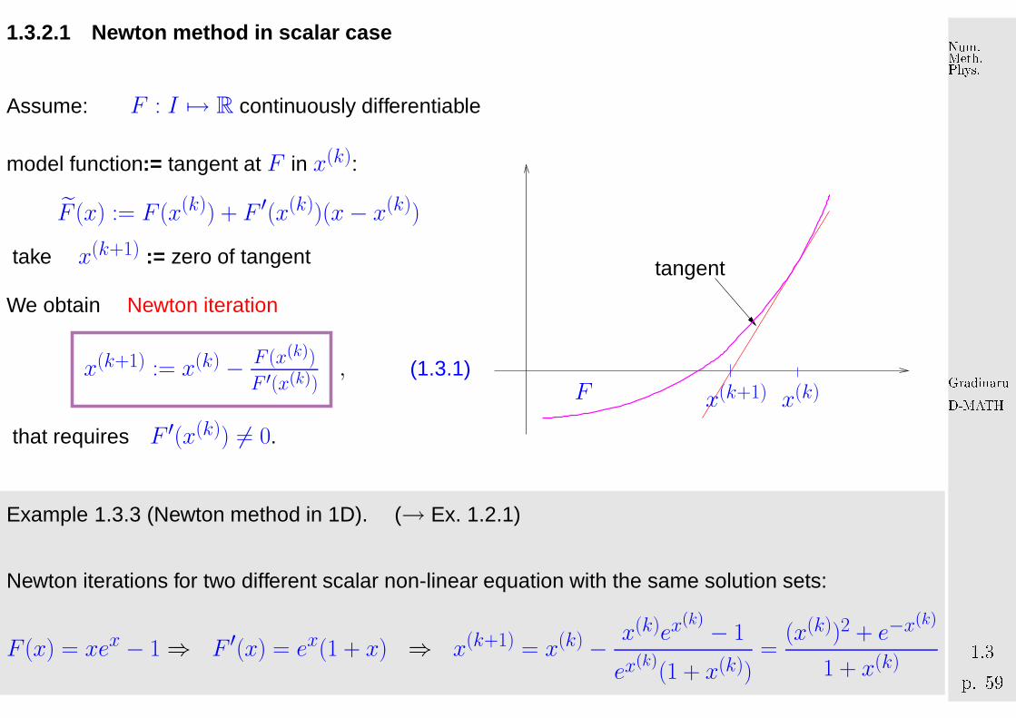
1.3.2.1 Newton method in sca lar case

Assume: F : I 7→ R continuously differentiable

model function:= tangent at F in x(k):

F̃ (x) := F (x(k)) + F ′(x(k))(x− x(k))

take x(k+1) := zero of tangent

We obtain Newton iteration

x(k+1) := x(k) − F (x(k))

F ′(x(k)), (1.3.1)

that requires F ′(x(k)) 6= 0.

x(k)x(k+1)F

tangent

Example 1.3.3 (Newton method in 1D). (→ Ex. 1.2.1)

Newton iterations for two different scalar non-linear equation with the same solution sets:

F (x) = xex − 1⇒ F ′(x) = ex(1 + x) ⇒ x(k+1) = x(k) − x(k)ex(k) − 1

ex(k)

(1 + x(k))=

(x(k))2 + e−x(k)

1 + x(k)


Num.Meth.Phys.

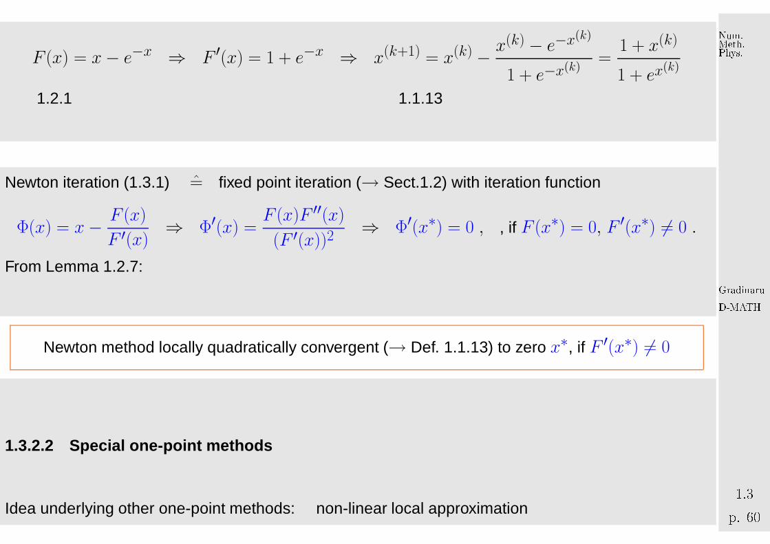
F (x) = x− e−x ⇒ F ′(x) = 1 + e−x ⇒ x(k+1) = x(k) − x(k) − e−x(k)

1 + e−x(k)=

1 + x(k)

1 + ex(k)

Ex. 1.2.1 shows quadratic convergence ! (→ Def. 1.1.13)3

Newton iteration (1.3.1) =̂ fixed point iteration (→ Sect.1.2) with iteration function

Φ(x) = x− F (x)

F ′(x)⇒ Φ′(x) =

F (x)F ′′(x)

(F ′(x))2⇒ Φ′(x∗) = 0 , , if F (x∗) = 0, F ′(x∗) 6= 0 .

From Lemma 1.2.7:

Newton method locally quadratically convergent (→ Def. 1.1.13) to zero x∗, if F ′(x∗) 6= 0

1.3.2.2 Special one-point method s

Idea underlying other one-point methods: non-linear local approximation


Num.Meth.Phys.

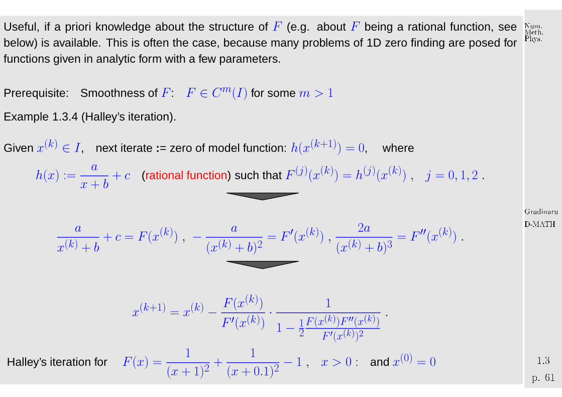
Useful, if a priori knowledge about the structure of F (e.g. about F being a rational function, seebelow) is available. This is often the case, because many problems of 1D zero finding are posed forfunctions given in analytic form with a few parameters.

Prerequisite: Smoothness of F : F ∈ Cm(I) for some m > 1

Example 1.3.4 (Halley’s iteration).

Given x(k) ∈ I , next iterate := zero of model function: h(x(k+1)) = 0, where

h(x) :=a

x + b+ c (rational function) such that F (j)(x(k)) = h(j)(x(k)) , j = 0, 1, 2 .

a

x(k) + b+ c = F (x(k)) , − a

(x(k) + b)2= F ′(x(k)) ,

2a

(x(k) + b)3= F ′′(x(k)) .

x(k+1) = x(k) − F (x(k))

F ′(x(k))· 1

1− 12F (x(k))F ′′(x(k))

F ′(x(k))2

.

Halley’s iteration for F (x) =1

(x + 1)2+

1

(x + 0.1)2− 1 , x > 0 : and x(0) = 0


Num.Meth.Phys.

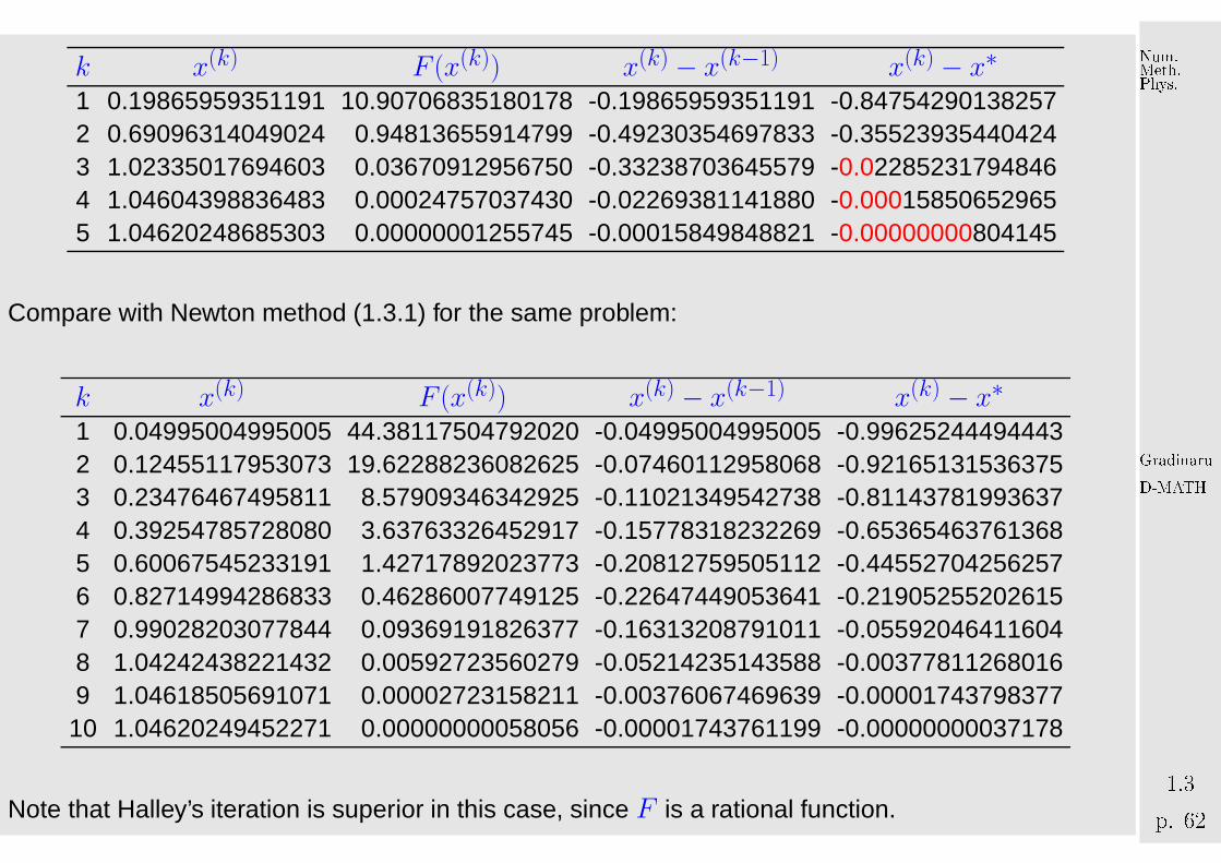
k x(k) F (x(k)) x(k) − x(k−1) x(k) − x∗1 0.19865959351191 10.90706835180178 -0.19865959351191 -0.847542901382572 0.69096314049024 0.94813655914799 -0.49230354697833 -0.355239354404243 1.02335017694603 0.03670912956750 -0.33238703645579 -0.022852317948464 1.04604398836483 0.00024757037430 -0.02269381141880 -0.000158506529655 1.04620248685303 0.00000001255745 -0.00015849848821 -0.00000000804145

Compare with Newton method (1.3.1) for the same problem:

k x(k) F (x(k)) x(k) − x(k−1) x(k) − x∗1 0.04995004995005 44.38117504792020 -0.04995004995005 -0.996252444944432 0.12455117953073 19.62288236082625 -0.07460112958068 -0.921651315363753 0.23476467495811 8.57909346342925 -0.11021349542738 -0.811437819936374 0.39254785728080 3.63763326452917 -0.15778318232269 -0.653654637613685 0.60067545233191 1.42717892023773 -0.20812759505112 -0.445527042562576 0.82714994286833 0.46286007749125 -0.22647449053641 -0.219052552026157 0.99028203077844 0.09369191826377 -0.16313208791011 -0.055920464116048 1.04242438221432 0.00592723560279 -0.05214235143588 -0.003778112680169 1.04618505691071 0.00002723158211 -0.00376067469639 -0.0000174379837710 1.04620249452271 0.00000000058056 -0.00001743761199 -0.00000000037178

Note that Halley’s iteration is superior in this case, since F is a rational function.


Num.Meth.Phys.

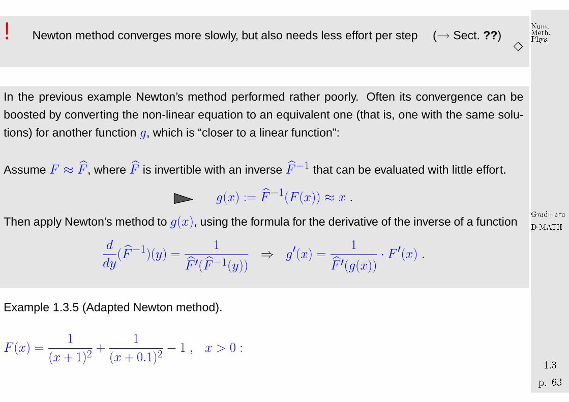
! Newton method converges more slowly, but also needs less effort per step (→ Sect. ?? )3

In the previous example Newton’s method performed rather poorly. Often its convergence can be

boosted by converting the non-linear equation to an equivalent one (that is, one with the same solu-

tions) for another function g, which is “closer to a linear function”:

Assume F ≈ F̂ , where F̂ is invertible with an inverse F̂−1 that can be evaluated with little effort.

g(x) := F̂−1(F (x)) ≈ x .

Then apply Newton’s method to g(x), using the formula for the derivative of the inverse of a function

d

dy(F̂−1)(y) =

1

F̂ ′(F̂−1(y))⇒ g′(x) =

1

F̂ ′(g(x))· F ′(x) .

Example 1.3.5 (Adapted Newton method).

F (x) =1

(x + 1)2+

1

(x + 0.1)2− 1 , x > 0 :


Num.Meth.Phys.

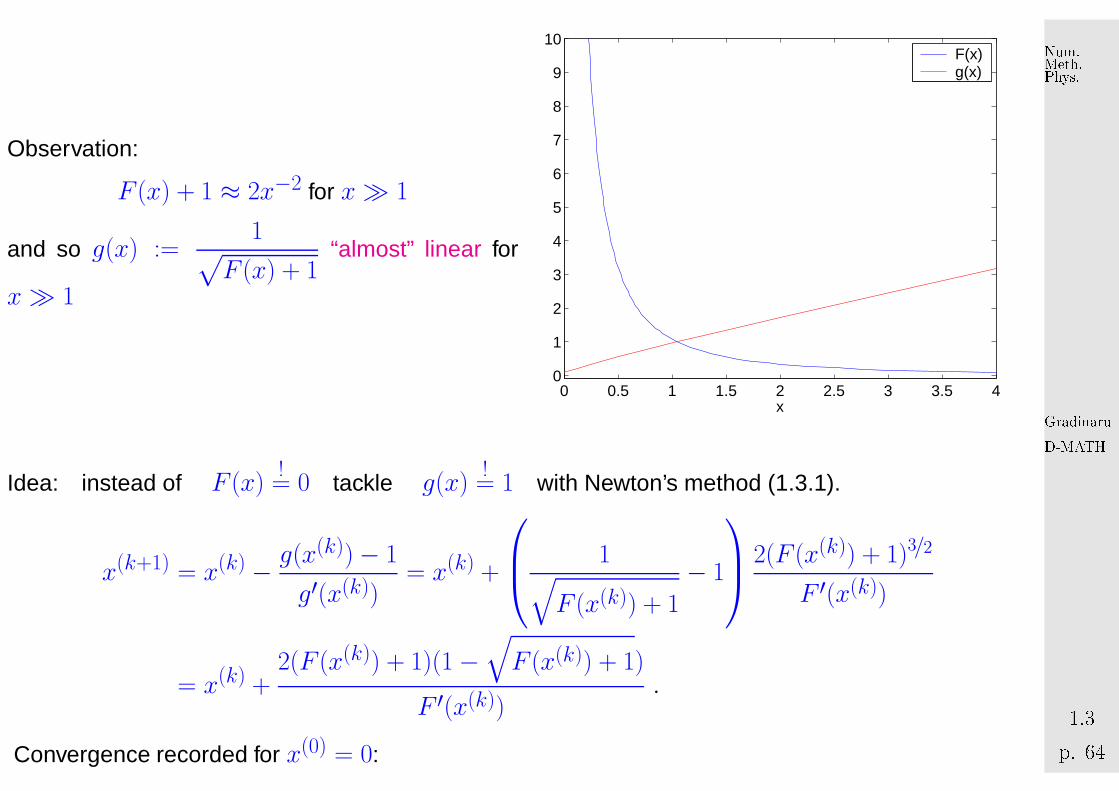
Observation:

F (x) + 1 ≈ 2x−2 for x≫ 1

and so g(x) :=1√

F (x) + 1“almost” linear for

x≫ 1

0 0.5 1 1.5 2 2.5 3 3.5 40

1

2

3

4

5

6

7

8

9

10

x

F(x)g(x)

Idea: instead of F (x)!= 0 tackle g(x)

!= 1 with Newton’s method (1.3.1).

x(k+1) = x(k) − g(x(k))− 1

g′(x(k))= x(k) +

1√F (x(k)) + 1

− 1

2(F (x(k)) + 1)3/2

F ′(x(k))

= x(k) +2(F (x(k)) + 1)(1−

√F (x(k)) + 1)

F ′(x(k)).

Convergence recorded for x(0) = 0:


Num.Meth.Phys.

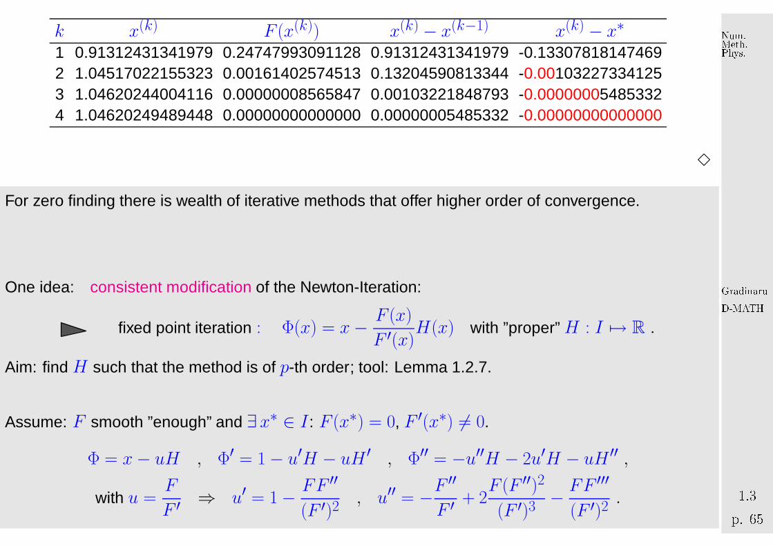
k x(k) F (x(k)) x(k) − x(k−1) x(k) − x∗1 0.91312431341979 0.24747993091128 0.91312431341979 -0.133078181474692 1.04517022155323 0.00161402574513 0.13204590813344 -0.001032273341253 1.04620244004116 0.00000008565847 0.00103221848793 -0.000000054853324 1.04620249489448 0.00000000000000 0.00000005485332 -0.00000000000000

3

For zero finding there is wealth of iterative methods that offer higher order of convergence.

One idea: consistent modification of the Newton-Iteration:

fixed point iteration : Φ(x) = x− F (x)

F ′(x)H(x) with ”proper” H : I 7→ R .

Aim: find H such that the method is of p-th order; tool: Lemma 1.2.7.

Assume: F smooth ”enough” and ∃ x∗ ∈ I : F (x∗) = 0, F ′(x∗) 6= 0.

Φ = x− uH , Φ′ = 1− u′H − uH ′ , Φ′′ = −u′′H − 2u′H − uH ′′ ,

with u =F

F ′⇒ u′ = 1− FF ′′

(F ′)2, u′′ = −F

′′

F ′+ 2

F (F ′′)2

(F ′)3− FF ′′′

(F ′)2.


Num.Meth.Phys.

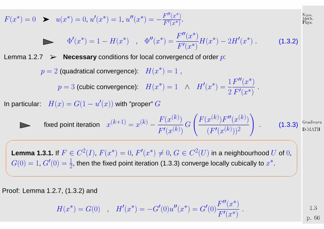
F (x∗) = 0 ➤ u(x∗) = 0, u′(x∗) = 1, u′′(x∗) = −F′′(x∗)

F ′(x∗) .

Φ′(x∗) = 1−H(x∗) , Φ′′(x∗) =F ′′(x∗)F ′(x∗)

H(x∗)− 2H ′(x∗) . (1.3.2)

Lemma 1.2.7 ➢ Necessa ry conditions for local convergencd of order p:

p = 2 (quadratical convergence): H(x∗) = 1 ,

p = 3 (cubic convergence): H(x∗) = 1 ∧ H ′(x∗) =1

2

F ′′(x∗)F ′(x∗)

.

In particular: H(x) = G(1− u′(x)) with ”proper” G

fixed point iteration x(k+1) = x(k) − F (x(k))

F ′(x(k))G

(F (x(k))F ′′(x(k))

(F ′(x(k)))2

). (1.3.3)

'

&

$

%

Lemma 1.3.1. If F ∈ C2(I), F (x∗) = 0, F ′(x∗) 6= 0, G ∈ C2(U ) in a neighbourhood U of 0,

G(0) = 1, G′(0) = 12, then the fixed point iteration (1.3.3) converge locally cubically to x∗.

Proof: Lemma 1.2.7, (1.3.2) and

H(x∗) = G(0) , H ′(x∗) = −G′(0)u′′(x∗) = G′(0)F ′′(x∗)F ′(x∗)

.


Num.Meth.Phys.

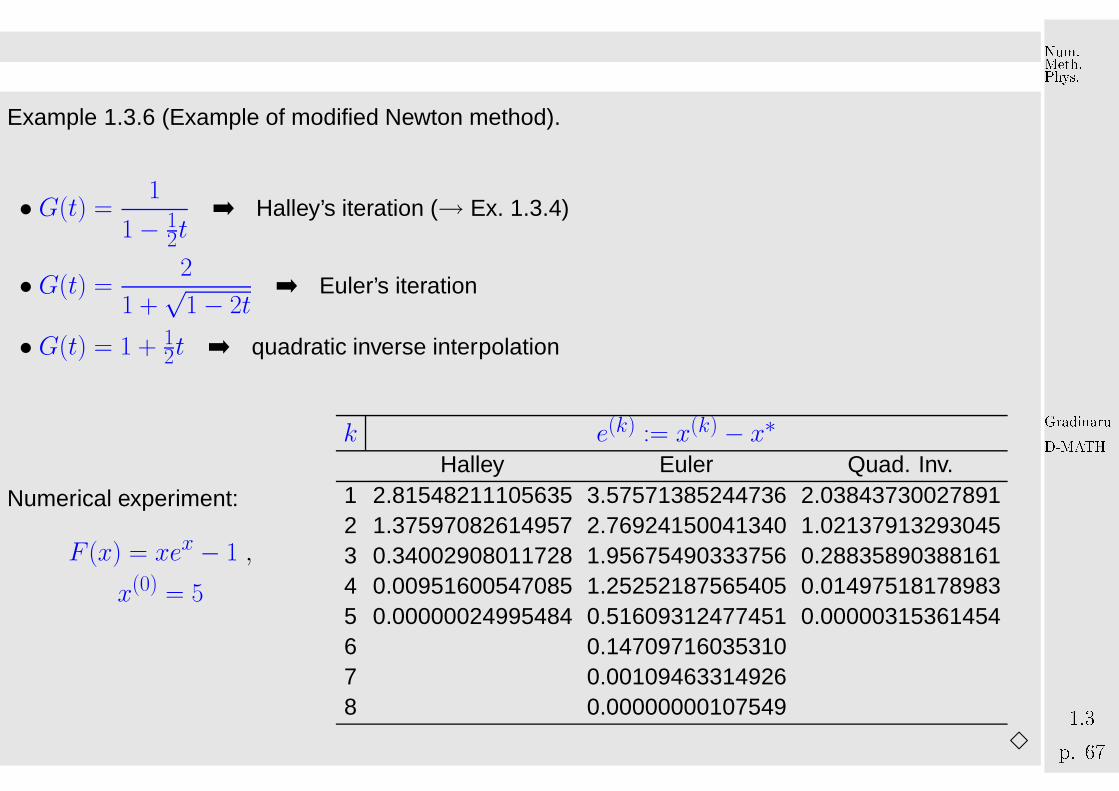
Example 1.3.6 (Example of modified Newton method).

• G(t) =1

1− 12t

➡ Halley’s iteration (→ Ex. 1.3.4)

• G(t) =2

1 +√

1− 2t➡ Euler’s iteration

• G(t) = 1 + 12t ➡ quadratic inverse interpolation

Numerical experiment:

F (x) = xex − 1 ,

x(0) = 5

k e(k) := x(k) − x∗Halley Euler Quad. Inv.

1 2.81548211105635 3.57571385244736 2.038437300278912 1.37597082614957 2.76924150041340 1.021379132930453 0.34002908011728 1.95675490333756 0.288358903881614 0.00951600547085 1.25252187565405 0.014975181789835 0.00000024995484 0.51609312477451 0.000003153614546 0.147097160353107 0.001094633149268 0.00000000107549

3


Num.Meth.Phys.

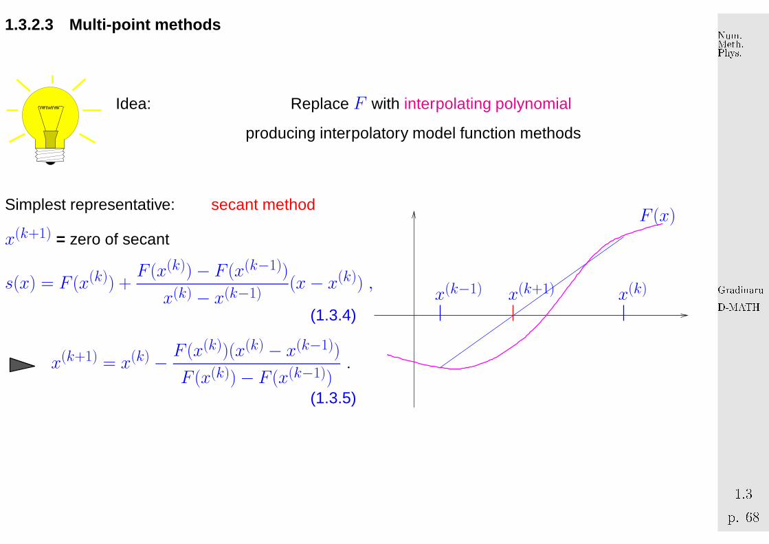
1.3.2.3 Multi-po int method s

Idea: Replace F with interpolating polynomial

producing interpolatory model function methods

Simplest representative: secant method

x(k+1) = zero of secant

s(x) = F (x(k)) +F (x(k))− F (x(k−1))

x(k) − x(k−1)(x− x(k)) ,

(1.3.4)

x(k+1) = x(k) − F (x(k))(x(k) − x(k−1))

F (x(k))− F (x(k−1)).

(1.3.5)

x(k−1) x(k)x(k+1)

F (x)


Num.Meth.Phys.

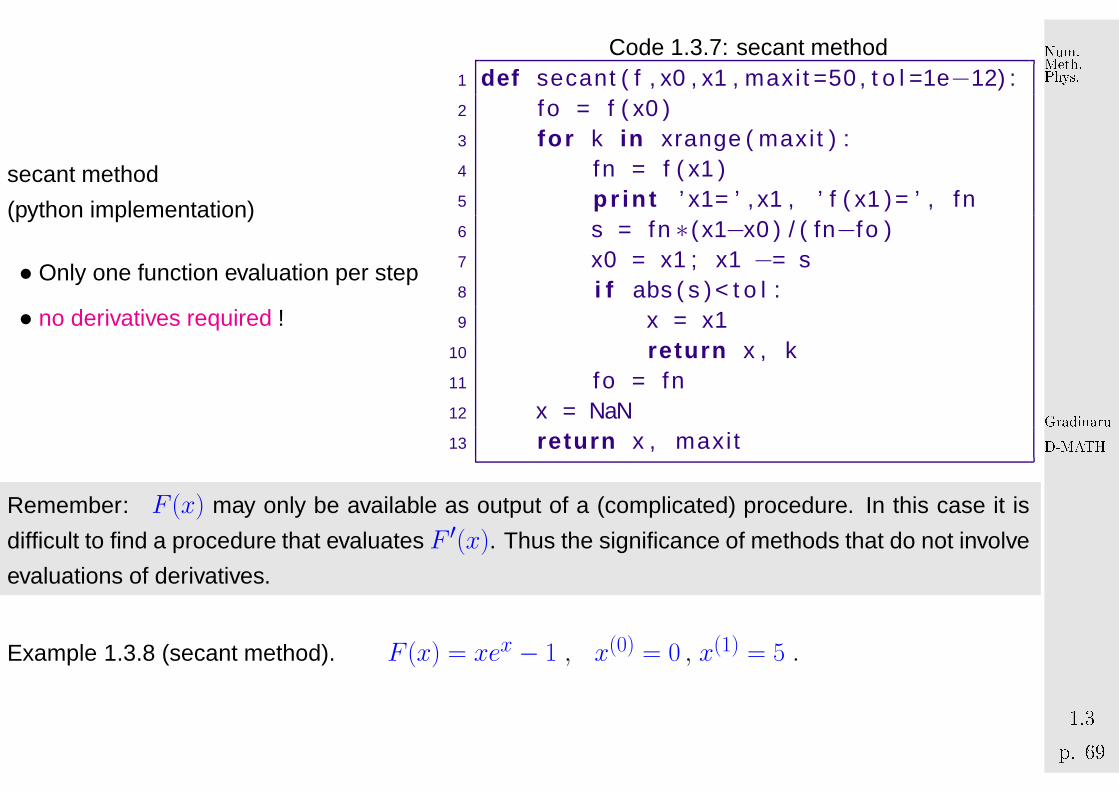
secant method

(python implementation)

• Only one function evaluation per step

• no derivatives required !

Code 1.3.7: secant method1 def secant ( f , x0 , x1 , maxi t =50 , t o l =1e−12) :2 fo = f ( x0 )3 f o r k i n xrange ( maxi t ) :4 fn = f ( x1 )5 p r i n t ’ x1= ’ , x1 , ’ f ( x1 ) = ’ , fn6 s = fn ∗( x1−x0 ) / ( fn−fo )7 x0 = x1 ; x1 −= s8 i f abs ( s ) < t o l :9 x = x1

10 r et u r n x , k11 fo = fn12 x = NaN13 r et u r n x , maxi t

Remember: F (x) may only be available as output of a (complicated) procedure. In this case it is

difficult to find a procedure that evaluates F ′(x). Thus the significance of methods that do not involve

evaluations of derivatives.

Example 1.3.8 (secant method). F (x) = xex − 1 , x(0) = 0 , x(1) = 5 .


Num.Meth.Phys.

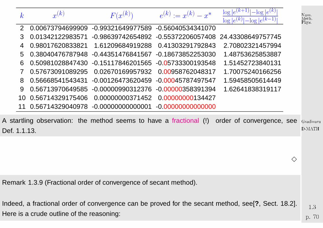
k x(k) F (x(k)) e(k) := x(k) − x∗ log |e(k+1)|−log |e(k)|log |e(k)|−log |e(k−1)|

2 0.00673794699909 -0.99321649977589 -0.560405343410703 0.01342122983571 -0.98639742654892 -0.55372206057408 24.433086497577454 0.98017620833821 1.61209684919288 0.41303291792843 2.708023214579945 0.38040476787948 -0.44351476841567 -0.18673852253030 1.487536258538876 0.50981028847430 -0.15117846201565 -0.05733300193548 1.514527238401317 0.57673091089295 0.02670169957932 0.00958762048317 1.700752401662568 0.56668541543431 -0.00126473620459 -0.00045787497547 1.594585056144499 0.56713970649585 -0.00000990312376 -0.00000358391394 1.6264183831911710 0.56714329175406 0.00000000371452 0.0000000013442711 0.56714329040978 -0.00000000000001 -0.00000000000000

A startling observation: the method seems to have a fractional (!) order of convergence, see

Def. 1.1.13.

3

Remark 1.3.9 (Fractional order of convergence of secant method).

Indeed, a fractional order of convergence can be proved for the secant method, see[?, Sect. 18.2].

Here is a crude outline of the reasoning:


Num.Meth.Phys.

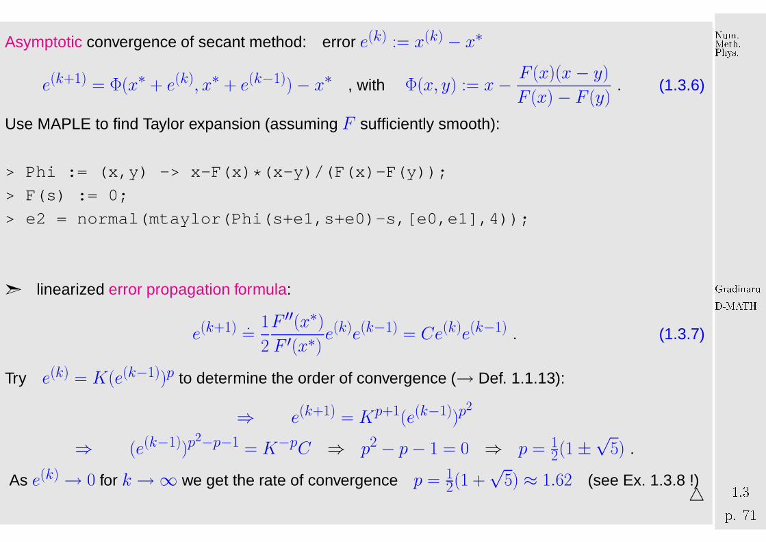
Asymptotic convergence of secant method: error e(k) := x(k) − x∗

e(k+1) = Φ(x∗ + e(k), x∗ + e(k−1))− x∗ , with Φ(x, y) := x− F (x)(x− y)F (x)− F (y)

. (1.3.6)

Use MAPLE to find Taylor expansion (assuming F sufficiently smooth):

> Phi := (x,y) -> x-F(x)*(x-y)/(F(x)-F(y));

> F(s) := 0;

> e2 = normal(mtaylor(Phi(s+e1,s+e0)-s,[e0,e1],4));

➣ linearized error propagation formula:

e(k+1) .=

1

2

F ′′(x∗)F ′(x∗)

e(k)e(k−1) = Ce(k)e(k−1) . (1.3.7)

Try e(k) = K(e(k−1))p to determine the order of convergence (→ Def. 1.1.13):

⇒ e(k+1) = Kp+1(e(k−1))p2

⇒ (e(k−1))p2−p−1 = K−pC ⇒ p2 − p− 1 = 0 ⇒ p = 1

2(1±√

5) .

As e(k)→ 0 for k →∞ we get the rate of convergence p = 12(1 +

√5) ≈ 1.62 (see Ex. 1.3.8 !)

△


Num.Meth.Phys.

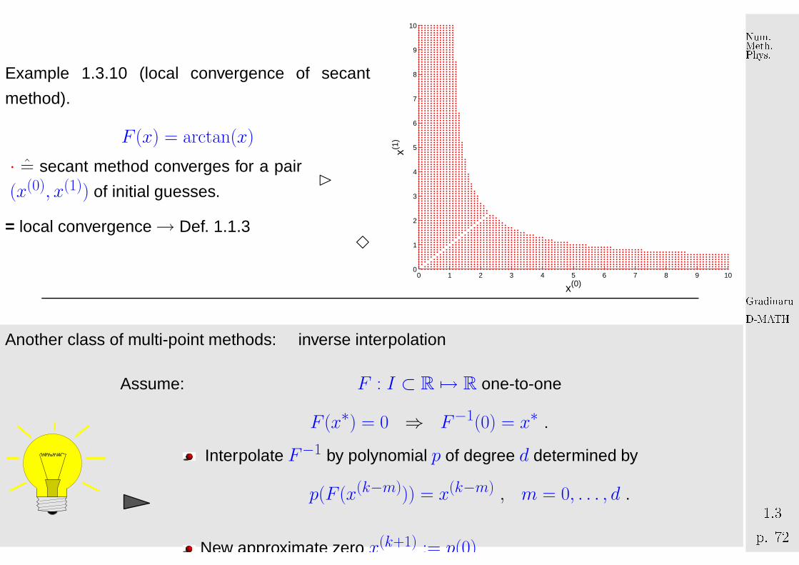
Example 1.3.10 (local convergence of secant

method).

F (x) = arctan(x)

· =̂ secant method converges for a pair

(x(0), x(1)) of initial guesses.�

= local convergence→ Def. 1.1.33

0 1 2 3 4 5 6 7 8 9 100

1

2

3

4

5

6

7

8

9

10

x(0)

x(1)

Another class of multi-point methods: inverse interpolation

Assume: F : I ⊂ R 7→ R one-to-one

F (x∗) = 0 ⇒ F−1(0) = x∗ .

Interpolate F−1 by polynomial p of degree d determined by

p(F (x(k−m))) = x(k−m) , m = 0, . . . , d .

New approximate zero x(k+1) := p(0)


Num.Meth.Phys.

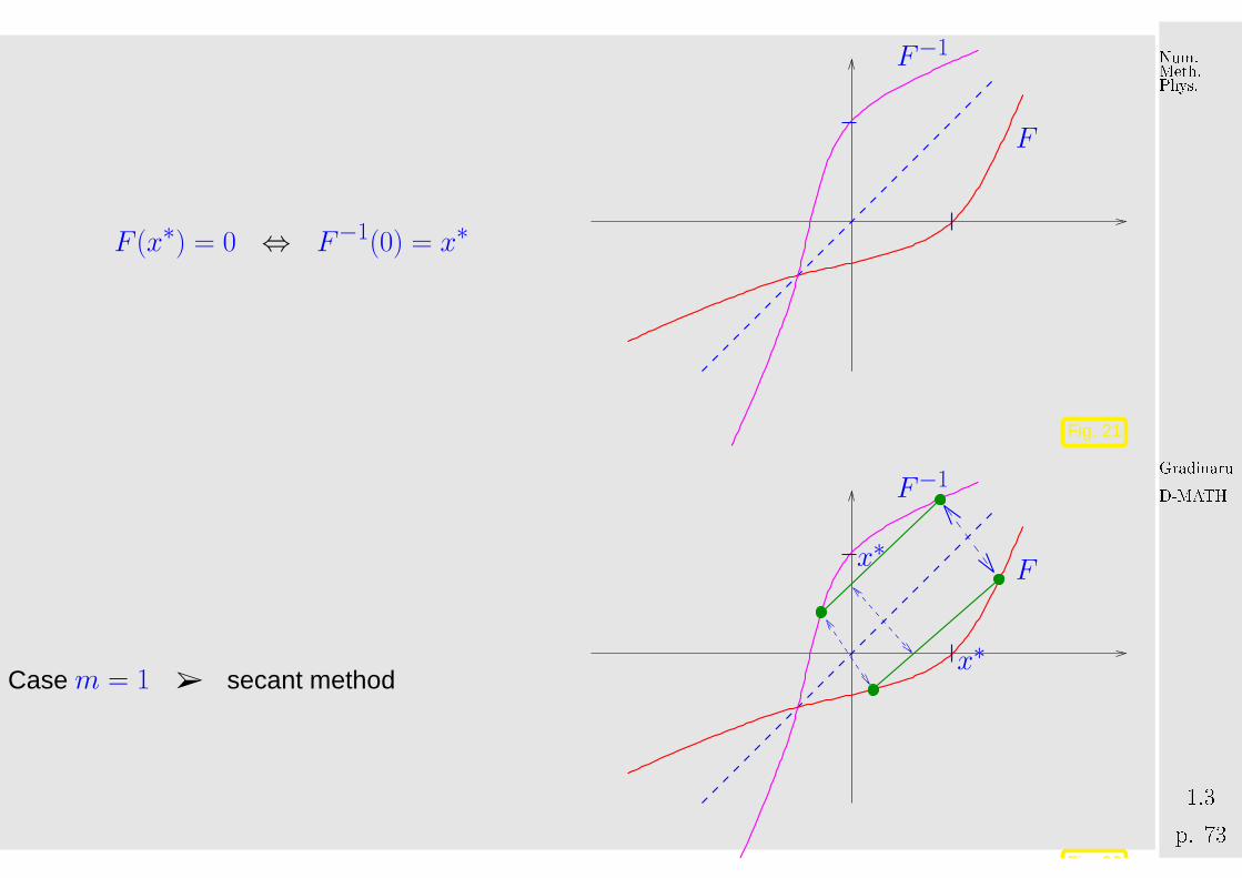
F (x∗) = 0 ⇔ F−1(0) = x∗

F−1

F

Fig. 21

Case m = 1 ➢ secant method

x∗

x∗

F−1

F

Fig. 22


Num.Meth.Phys.

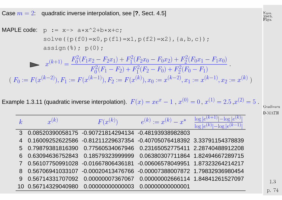
Case m = 2: quadratic inverse interpolation, see [?, Sect. 4.5]

MAPLE code: p := x-> a*x^2+b*x+c;

solve({p(f0)=x0,p(f1)=x1,p(f2)=x2},{a,b,c});

assign(%); p(0);

x(k+1) =F 2

0 (F1x2 − F2x1) + F 21 (F2x0 − F0x2) + F 2

2 (F0x1 − F1x0)

F 20 (F1 − F2) + F 2

1 (F2 − F0) + F 22 (F0 − F1)

.

( F0 := F (x(k−2)), F1 := F (x(k−1)), F2 := F (x(k)), x0 := x(k−2), x1 := x(k−1), x2 := x(k) )

Example 1.3.11 (quadratic inverse interpolation). F (x) = xex − 1 , x(0) = 0 , x(1) = 2.5 ,x(2) = 5 .

k x(k) F (x(k)) e(k) := x(k) − x∗ log |e(k+1)|−log |e(k)|log |e(k)|−log |e(k−1)|

3 0.08520390058175 -0.90721814294134 -0.481939389828034 0.16009252622586 -0.81211229637354 -0.40705076418392 3.337911543788395 0.79879381816390 0.77560534067946 0.23165052775411 2.287404889122086 0.63094636752843 0.18579323999999 0.06380307711864 1.824946672897157 0.56107750991028 -0.01667806436181 -0.00606578049951 1.873232642142178 0.56706941033107 -0.00020413476766 -0.00007388007872 1.798329369804549 0.56714331707092 0.00000007367067 0.00000002666114 1.84841261527097

10 0.56714329040980 0.00000000000003 0.00000000000001


Num.Meth.Phys.

Also in this case the numerical experiment hints at a fractional rate of convergence, as in the case of

the secant method, see Rem. 1.3.9.

3

1.4 Newton’s Method

Non-linear system of equations: for F : D ⊂ Rn 7→ Rn find x∗ ∈ D: F (x∗) = 0

Assume: F : D ⊂ Rn 7→ R

n continuously differentiable


Num.Meth.Phys.

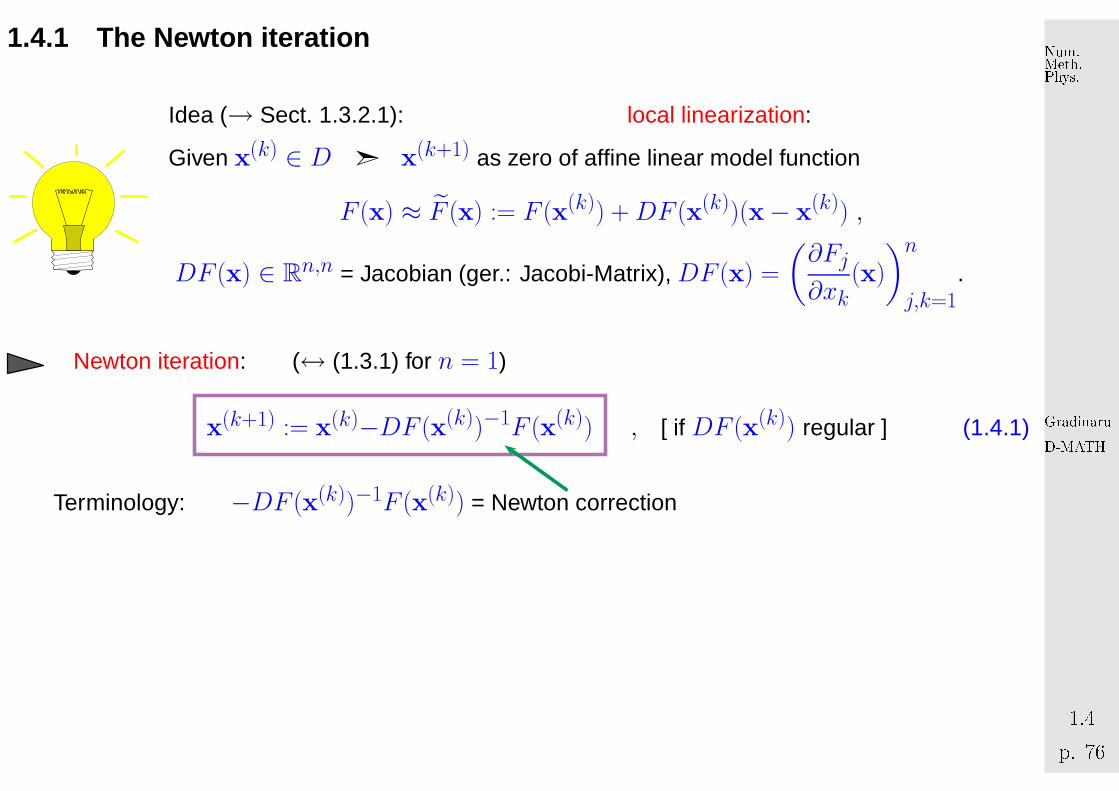
1.4.1 The Newton iteration

Idea (→ Sect. 1.3.2.1): local linearization:

Given x(k) ∈ D ➣ x(k+1) as zero of affine linear model function

F (x) ≈ F̃ (x) := F (x(k)) +DF (x(k))(x− x(k)) ,

DF (x) ∈ Rn,n = Jacobian (ger.: Jacobi-Matrix), DF (x) =

(∂Fj∂xk

(x)

)n

j,k=1.

Newton iteration: (↔ (1.3.1) for n = 1)

x(k+1) := x(k)−DF (x(k))−1F (x(k)) , [ if DF (x(k)) regular ] (1.4.1)

Terminology: −DF (x(k))−1F (x(k)) = Newton correction


Num.Meth.Phys.

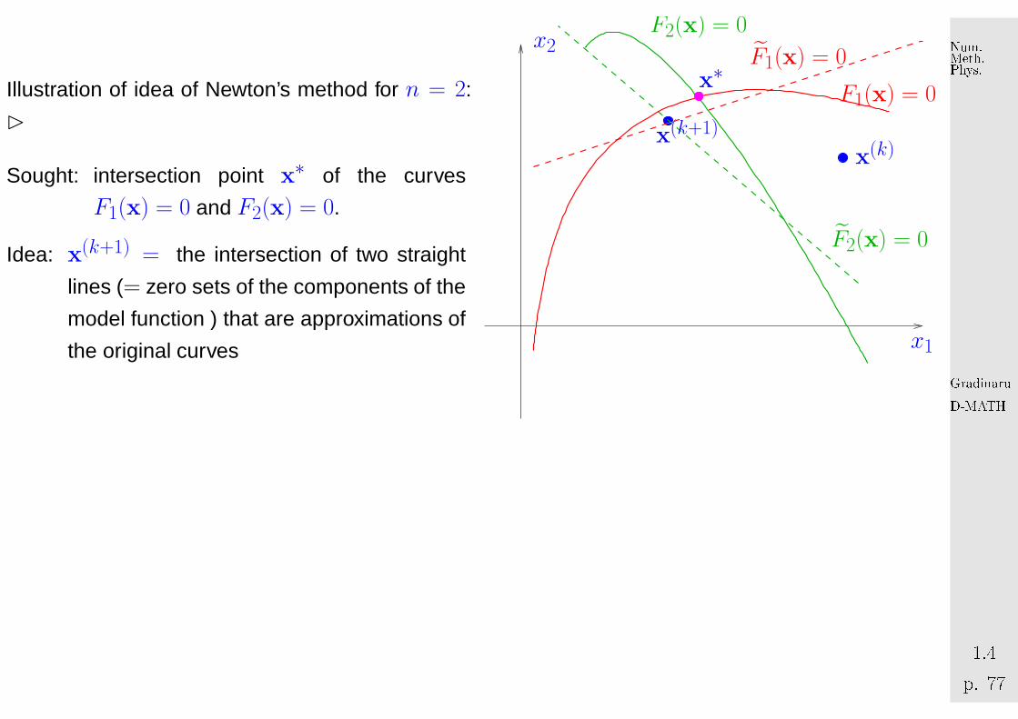
Illustration of idea of Newton’s method for n = 2:

�

Sought: intersection point x∗ of the curves

F1(x) = 0 and F2(x) = 0.

Idea: x(k+1) = the intersection of two straight

lines (= zero sets of the components of the

model function ) that are approximations of

the original curves

x∗

x1

x2

x(k)x(k+1)

F1(x) = 0

F2(x) = 0

F̃2(x) = 0

F̃1(x) = 0GradinaruD-MATH


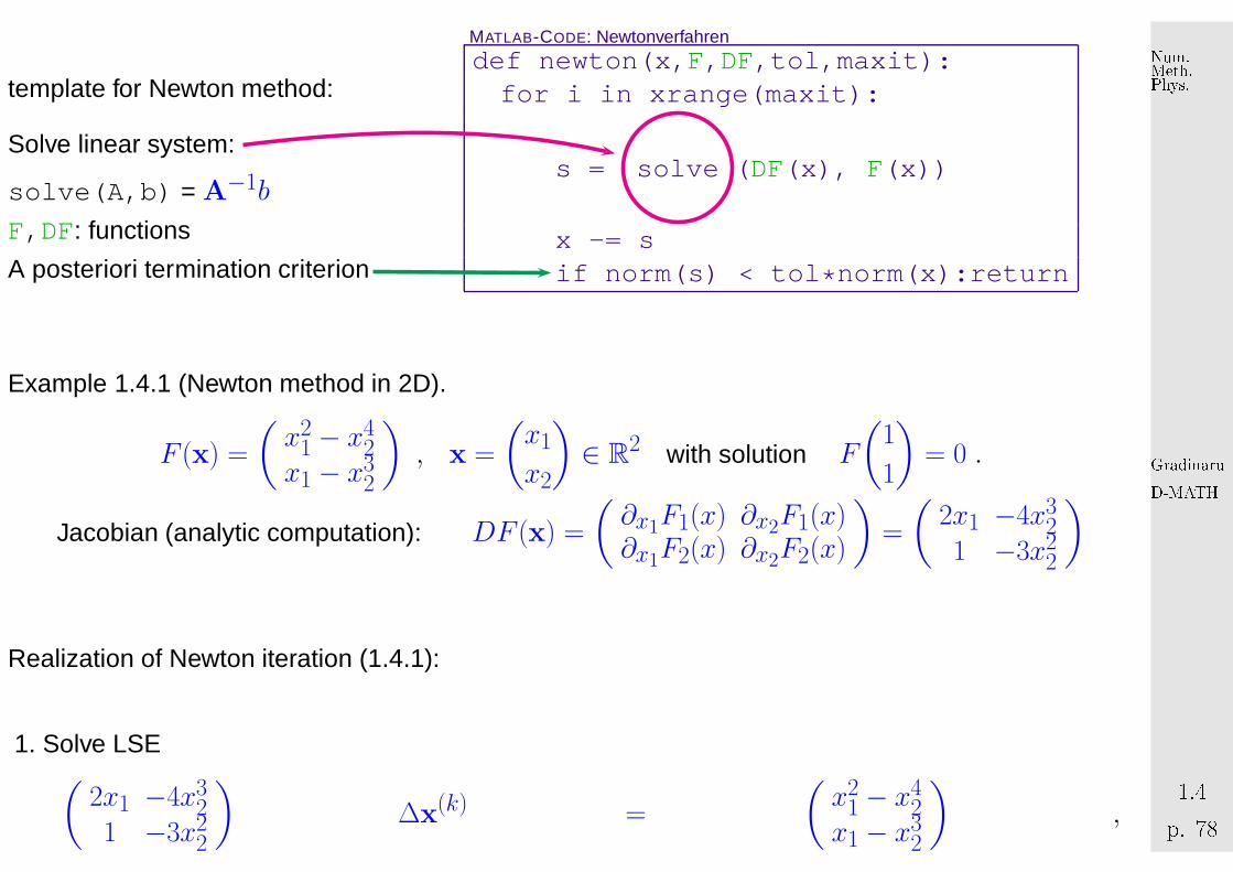
template for Newton method:

Solve linear system:

solve(A,b) = A−1b

F,DF: functions

A posteriori termination criterion

MATLAB-CODE: Newtonverfahren

def newton(x,F,DF,tol,maxit):for i in xrange(maxit):

s = solve (DF(x), F(x))

x -= sif norm(s) < tol*norm(x):return

Example 1.4.1 (Newton method in 2D).

F (x) =

(x2

1 − x42

x1 − x32

), x =

(x1

x2

)∈ R

2 with solution F

(1

1

)= 0 .

Jacobian (analytic computation): DF (x) =

(∂x1F1(x) ∂x2F1(x)∂x1F2(x) ∂x2F2(x)

)=

(2x1 −4x3

21 −3x2

2

)

Realization of Newton iteration (1.4.1):

1. Solve LSE(

2x1 −4x32

1 −3x22

)∆x(k) =

(x2

1 − x42

x1 − x32

),


Num.Meth.Phys.

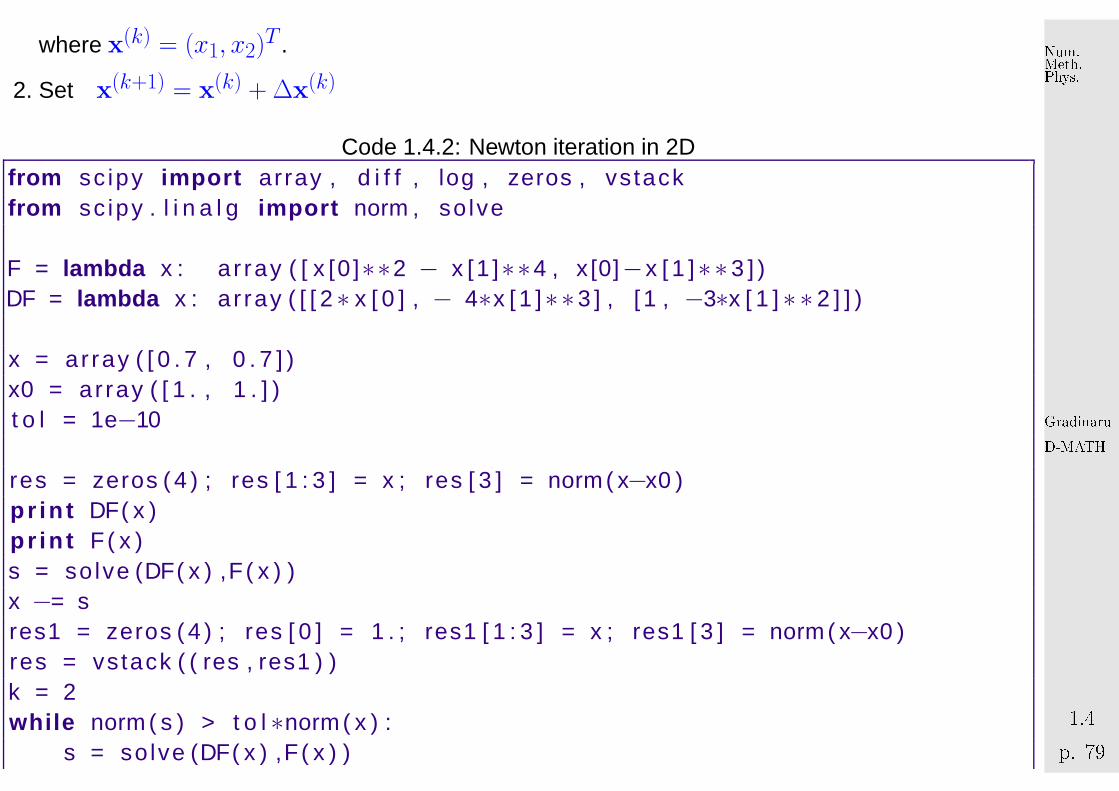
where x(k) = (x1, x2)T .

2. Set x(k+1) = x(k) + ∆x(k)

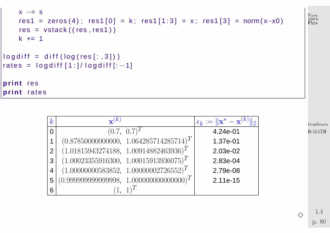
Code 1.4.2: Newton iteration in 2D1 from sc ipy impo r t array , d i f f , log , zeros , vstack2 from sc ipy . l i n a l g impo r t norm , so lve3

4 F = lambda x : a r ray ( [ x [0 ]∗∗2 − x [1 ]∗∗4 , x [0]−x [ 1 ]∗∗3 ] )5 DF = lambda x : a r ray ( [ [ 2∗ x [ 0 ] , − 4∗x [ 1 ]∗∗3 ] , [ 1 , −3∗x [ 1 ] ∗ ∗ 2 ] ] )6

7 x = ar ray ( [ 0 . 7 , 0 . 7 ] )8 x0 = ar ray ( [ 1 . , 1 . ] )9 t o l = 1e−100

1 res = zeros ( 4 ) ; res [ 1 : 3 ] = x ; res [ 3 ] = norm ( x−x0 )2 p r i n t DF( x )3 p r i n t F( x )4 s = so lve (DF( x ) ,F ( x ) )5 x −= s6 res1 = zeros ( 4 ) ; res [ 0 ] = 1 . ; res1 [ 1 : 3 ] = x ; res1 [ 3 ] = norm ( x−x0 )7 res = vstack ( ( res , res1 ) )8 k = 29 w h il e norm ( s ) > t o l ∗norm ( x ) :0 s = so lve (DF( x ) ,F ( x ) )


Num.Meth.Phys.

1 x −= s2 res1 = zeros ( 4 ) ; res1 [ 0 ] = k ; res1 [ 1 : 3 ] = x ; res1 [ 3 ] = norm ( x−x0 )3 res = vstack ( ( res , res1 ) )4 k += 15

6 l o g d i f f = d i f f ( log ( res [ : , 3 ] ) )7 r a tes = l o g d i f f [ 1 : ] / l o g d i f f [ :−1]8

9 p r i n t res0 p r i n t r a tes

k x(k) ǫk := ‖x∗ − x(k)‖20 (0.7, 0.7)T 4.24e-011 (0.87850000000000, 1.064285714285714)T 1.37e-012 (1.01815943274188, 1.00914882463936)T 2.03e-023 (1.00023355916300, 1.00015913936075)T 2.83e-044 (1.00000000583852, 1.00000002726552)T 2.79e-085 (0.999999999999998, 1.000000000000000)T 2.11e-156 (1, 1)T

3


Num.Meth.Phys.

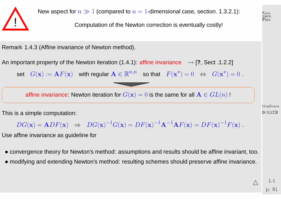
!New aspect for n≫ 1 (compared to n = 1-dimensional case, section. 1.3.2.1):

Computation of the Newton correction is eventually costly!

Remark 1.4.3 (Affine invariance of Newton method).

An important property of the Newton iteration (1.4.1): affine invariance → [?, Sect .1.2.2]

set G(x) := AF (x) with regular A ∈ Rn,n so that F (x∗) = 0 ⇔ G(x∗) = 0 .

��

��affine invariance: Newton iteration for G(x) = 0 is the same for all A ∈ GL(n) !

This is a simple computation:

DG(x) = ADF (x) ⇒ DG(x)−1G(x) = DF (x)−1A−1AF (x) = DF (x)−1F (x) .

Use affine invariance as guideline for

• convergence theory for Newton’s method: assumptions and results should be affine invariant, too.

• modifying and extending Newton’s method: resulting schemes should preserve affine invariance.

△


Num.Meth.Phys.

Remark 1.4.4 (Differentiation rules). → Repetition: basic analysis

Statement of the Newton iteration (1.4.1) for F : Rn 7→ R

n given as analytic expression entails

computing the Jacobian DF . To avoid cumbersome component-oriented considerations, it is useful

to know the rules of multidimensional differentiation:

Let V , W be finite dimensional vector spaces, F : D ⊂ V 7→ W sufficiently smooth. The differential

DF (x) of F in x ∈ V is the unique

linear mapping DF (x) : V 7→ W ,

such that ‖F (x + h)− F (x)−DF (h)h‖ = o(‖h‖) ∀h , ‖h‖ < δ .

• For F : V 7→ W linear, i.e. F (x) = Ax, A matrix ➤ DF (x) = A.

• Chain rule: F : V 7→ W , G : W 7→ U sufficiently smooth

D(G ◦ F )(x)h = DG(F (x))(DF (x))h , h ∈ V , x ∈ D . (1.4.2)


Num.Meth.Phys.

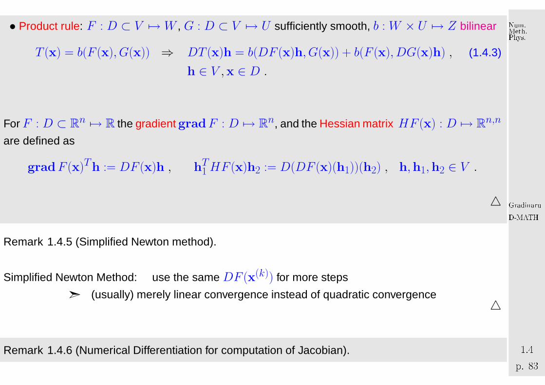
• Product rule: F : D ⊂ V 7→ W , G : D ⊂ V 7→ U sufficiently smooth, b : W × U 7→ Z bilinear

T (x) = b(F (x), G(x)) ⇒ DT (x)h = b(DF (x)h, G(x)) + b(F (x), DG(x)h) ,

h ∈ V ,x ∈ D .

(1.4.3)

For F : D ⊂ Rn 7→ R the gradient gradF : D 7→ R

n, and the Hessian matrix HF (x) : D 7→ Rn,n

are defined as

gradF (x)Th := DF (x)h , hT1 HF (x)h2 := D(DF (x)(h1))(h2) , h,h1,h2 ∈ V .

△

Remark 1.4.5 (Simplified Newton method).

Simplified Newton Method: use the same DF (x(k)) for more steps

➣ (usually) merely linear convergence instead of quadratic convergence△

Remark 1.4.6 (Numerical Differentiation for computation of Jacobian).


Num.Meth.Phys.

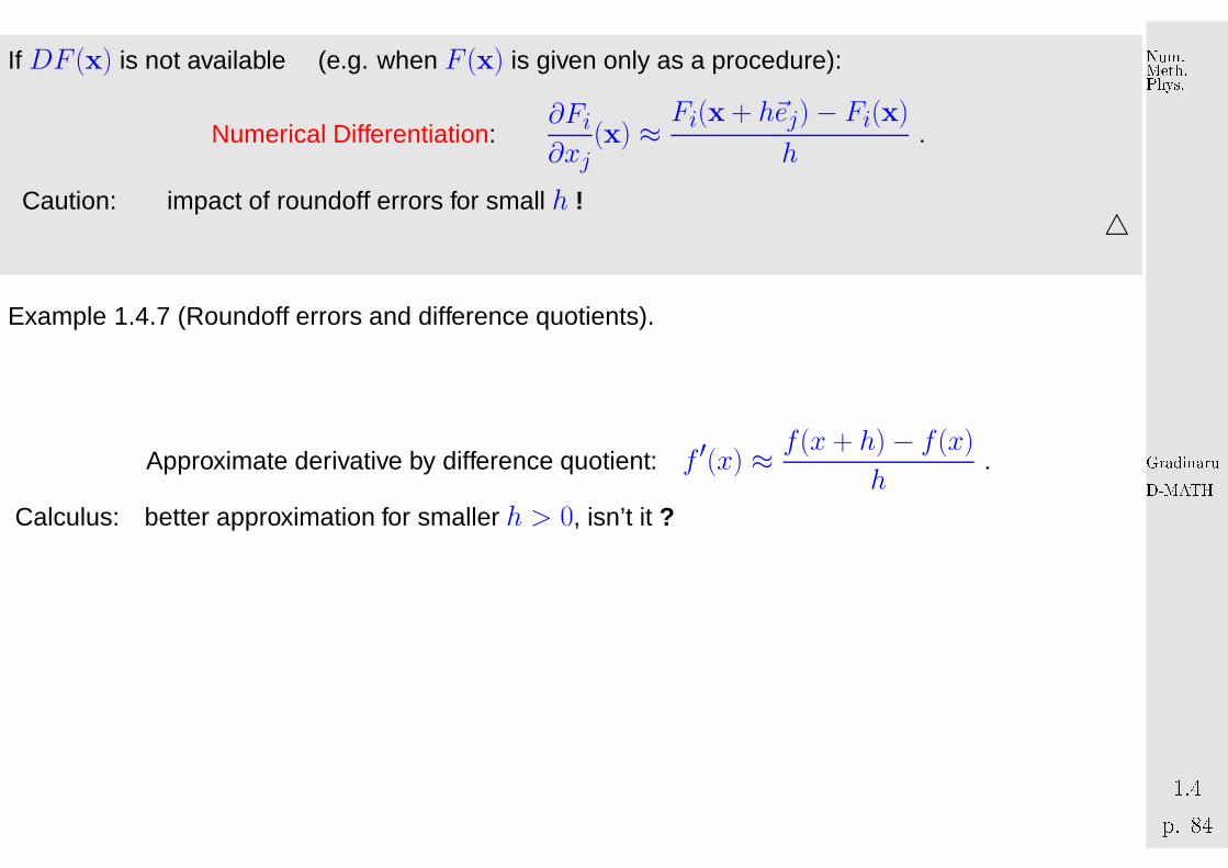
If DF (x) is not available (e.g. when F (x) is given only as a procedure):

Numerical Differentiation:∂Fi∂xj

(x) ≈ Fi(x + h~ej)− Fi(x)

h.

Caution: impact of roundoff errors for small h !△

Example 1.4.7 (Roundoff errors and difference quotients).

Approximate derivative by difference quotient: f ′(x) ≈ f(x + h)− f(x)

h.

Calculus: better approximation for smaller h > 0, isn’t it ?


Num.Meth.Phys.

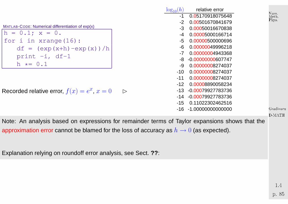
MATLAB-CODE: Numerical differentiation of exp(x)

h = 0.1; x = 0.for i in xrange(16):

df = (exp(x+h)-exp(x))/hprint -i, df-1h *= 0.1

Recorded relative error, f(x) = ex, x = 0 �

log10(h) relative error-1 0.05170918075648-2 0.00501670841679-3 0.00050016670838-4 0.00005000166714-5 0.00000500000696-6 0.00000049996218-7 0.00000004943368-8 -0.00000000607747-9 0.00000008274037

-10 0.00000008274037-11 0.00000008274037-12 0.00008890058234-13 -0.00079927783736-14 -0.00079927783736-15 0.11022302462516-16 -1.00000000000000

Note: An analysis based on expressions for remainder terms of Taylor expansions shows that the

approximation error cannot be blamed for the loss of accuracy as h→ 0 (as expected).

Explanation relying on roundoff error analysis, see Sect. ?? :


Num.Meth.Phys.

MATLAB-CODE: Numerical differentiation of exp(x)

h = 0.1; x = 0.0for i in xrange(16):

df = (exp(x+h)-exp(x)) /h

print -i, df-1h *= 0.1

Obvious cancellation→ error amplification

f ′(x)− f(x + h)− f(x)

h→ 0

Impact of roundoff→∞

for h→ 0 .

log10(h) relative error-1 0.05170918075648-2 0.00501670841679-3 0.00050016670838-4 0.00005000166714-5 0.00000500000696-6 0.00000049996218-7 0.00000004943368-8 -0.00000000607747-9 0.00000008274037

-10 0.00000008274037-11 0.00000008274037-12 0.00008890058234-13 -0.00079927783736-14 -0.00079927783736-15 0.11022302462516-16 -1.00000000000000

Analysis for f(x) = exp(x):

df =ex+h (1 + δ1) − ex (1 + δ2)

h

= ex

(eh − 1

h+δ1e

h − δ2h

)

correction factors take into account roundoff:

(→ "‘axiom of roundoff analysis”, Ass. ?? )

|δ1|, |δ2| ≤ eps .

1 +O(h) O(h−1) für h→ 0


Num.Meth.Phys.

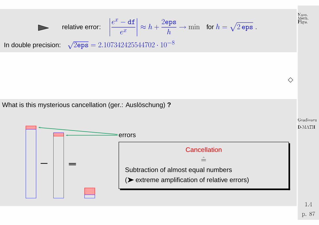
relative error:

∣∣∣∣ex − df

ex

∣∣∣∣ ≈ h +2eps

h→ min for h =

√2 eps .

In double precision:√

2eps = 2.107342425544702 · 10−8

3

What is this mysterious cancellation (ger.: Auslöschung) ?

errors

Cancellation

=̂

Subtraction of almost equal numbers

(➤ extreme amplification of relative errors)


Num.Meth.Phys.

Example 1.4.8 (cancellation in decimal floating point arithmetic).

x, y afflicted with relative errors≈ 10−7:

x = 0.123467∗ ← 7th digit perturbedy = 0.123456∗ ← 7th digit perturbed

x− y = 0.000011∗ = 0.11∗000 · 10−4 ← 3rd digit perturbed

padded zeroes

3

1.4.2 Convergence of Newton’s method

Newton iteration (1.4.1) =̂ fixed point iteration (→ Sect. 1.2) with

Φ(x) = x−DF (x)−1F (x) .

[“product rule” : DΦ(x) = I−D(DF (x)−1)F (x)−DF (x)−1DF (x) ]


Num.Meth.Phys.

F (x∗) = 0 ⇒ DΦ(x∗) = 0 .

Lemma 1.2.7 suggests conjecture:

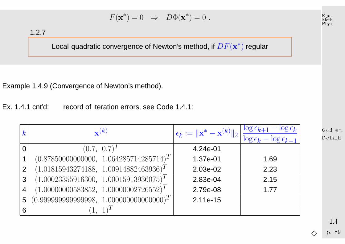
Local quadratic convergence of Newton’s method, if DF (x∗) regular

Example 1.4.9 (Convergence of Newton’s method).

Ex. 1.4.1 cnt’d: record of iteration errors, see Code 1.4.1:

k x(k) ǫk := ‖x∗ − x(k)‖2log ǫk+1 − log ǫklog ǫk − log ǫk−1

0 (0.7, 0.7)T 4.24e-011 (0.87850000000000, 1.064285714285714)T 1.37e-01 1.692 (1.01815943274188, 1.00914882463936)T 2.03e-02 2.233 (1.00023355916300, 1.00015913936075)T 2.83e-04 2.154 (1.00000000583852, 1.00000002726552)T 2.79e-08 1.775 (0.999999999999998, 1.000000000000000)T 2.11e-156 (1, 1)T

3


Num.Meth.Phys.

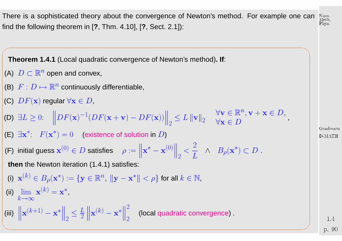
There is a sophisticated theory about the convergence of Newton’s method. For example one can

find the following theorem in [?, Thm. 4.10], [?, Sect. 2.1]):

'

&

$

%

Theorem 1.4.1 (Local quadratic convergence of Newton’s method). If:

(A) D ⊂ Rn open and convex,

(B) F : D 7→ Rn continuously differentiable,

(C) DF (x) regular ∀x ∈ D,

(D) ∃L ≥ 0:∥∥∥DF (x)−1(DF (x + v)−DF (x))

∥∥∥2≤ L ‖v‖2

∀v ∈ Rn,v + x ∈ D,∀x ∈ D ,

(E) ∃x∗: F (x∗) = 0 (existence of solution in D)

(F) initial guess x(0) ∈ D satisfies ρ :=∥∥∥x∗ − x(0)

∥∥∥2<

2

L∧ Bρ(x

∗) ⊂ D .

then the Newton iteration (1.4.1) satisfies:

(i) x(k) ∈ Bρ(x∗) := {y ∈ Rn, ‖y − x∗‖ < ρ} for all k ∈ N,

(ii) limk→∞

x(k) = x∗,

(iii)∥∥∥x(k+1) − x∗

∥∥∥2≤ L

2

∥∥∥x(k) − x∗∥∥∥

2

2(local quadratic convergence) .


Num.Meth.Phys.

✎ notation: ball Bρ(z) := {x ∈ Rn: ‖x− z‖2 ≤ ρ}

Terminology: (D) =̂ affine invariant Lipschitz condition

Problem: Usually neither ω nor x∗ are known !

In general: a priori estimates as in Thm. 1.4.1 are of little practical relevance.

1.4.3 Termination o f Newton iteration

A first viable idea:

Asymptotically due to quadratic convergence:∥∥∥x(k+1) − x∗

∥∥∥≪∥∥∥x(k) − x∗

∥∥∥ ⇒∥∥∥x(k) − x∗

∥∥∥ ≈∥∥∥x(k+1) − x(k)

∥∥∥ . (1.4.4)


Num.Meth.Phys.

➣ quit iterating as soon as∥∥∥x(k+1) − x(k)

∥∥∥ =∥∥∥DF (x(k))−1F (x(k))

∥∥∥ < τ∥∥∥x(k)

∥∥∥,

with τ = tolerance

→ uneconomical: one needless update, because x(k) already accurate enough !

Remark 1.4.10. New aspect for n≫ 1: computation of Newton correction may be expensive !△

Therefore we would like to use an a-posteriori termination criterion that dispenses with computing

(and “inverting”) another Jacobian DF (x(k)) just to tell us that x(k) is already accurate enough.

Practical a-posteriori termination criterion for Newton’s method:

DF (x(k−1)) ≈ DF (x(k)): quit as soon as∥∥∥DF (x(k−1))−1F (x(k))

∥∥∥ < τ∥∥∥x(k)

∥∥∥

affine invariant termination criterion

Justification: we expect DF (x(k−1)) ≈ DF (x(k)), when Newton iteration has converged. Then

appeal to (1.4.4).


Num.Meth.Phys.

If we used the residual based termination criterion∥∥∥F (x(k))

∥∥∥ ≤ τ ,

then the resulting algorithm would not be affine invariant, because for F (x) = 0 and AF (x) = 0,

A ∈ Rn,n regular, the Newton iteration might terminate with different iterates.

Terminology: ∆x̄(k) := DF (x(k−1))−1F (x(k)) =̂ simplified Newton correction

Reuse of LU-factorization of DF (x(k−1)) ➤∆x̄(k) available

with O(n2) operations

Summary: The Newton Method

converges asymptotically very fast: doubling of number of significant digits in each step

often a very small region of convergence, which requires an initial guess

rather close to the solution.


Num.Meth.Phys.

1.4.4 Damped Newton method

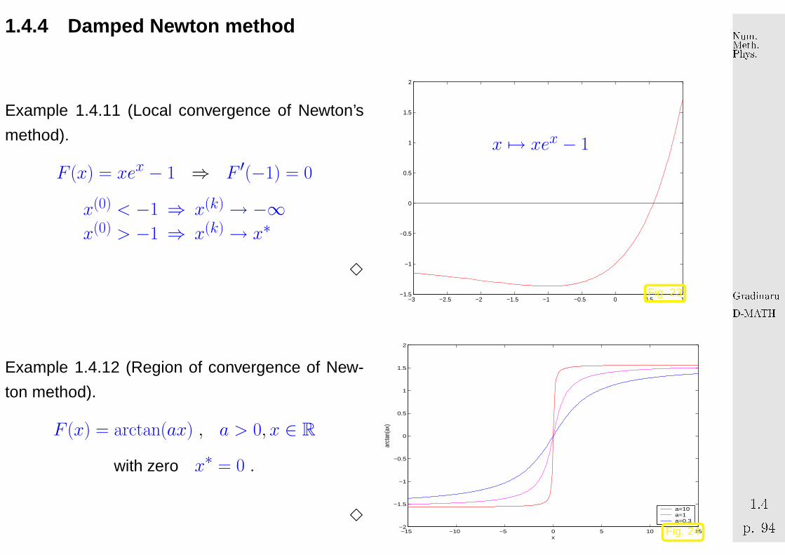
Example 1.4.11 (Local convergence of Newton’s

method).

F (x) = xex − 1 ⇒ F ′(−1) = 0

x(0) < −1 ⇒ x(k) → −∞x(0) > −1 ⇒ x(k) → x∗

3

−3 −2.5 −2 −1.5 −1 −0.5 0 0.5 1−1.5

−1

−0.5

0

0.5

1

1.5

2

x 7→ xex − 1

Fig. 23

Example 1.4.12 (Region of convergence of New-

ton method).

F (x) = arctan(ax) , a > 0, x ∈ R

with zero x∗ = 0 .

3−15 −10 −5 0 5 10 15

−2

−1.5

−1

−0.5

0

0.5

1

1.5

2

x

arct

an(a

x)

a=10a=1a=0.3

Fig. 24


Num.Meth.Phys.

−6 −4 −2 0 2 4 6−1.5

−1

−0.5

0

0.5

1

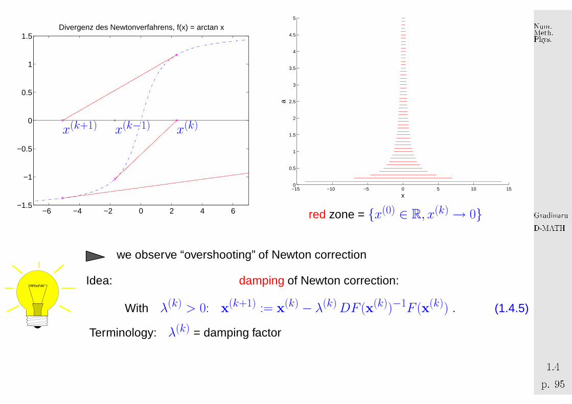
1.5Divergenz des Newtonverfahrens, f(x) = arctan x

x(k−1) x(k)x(k+1)

−15 −10 −5 0 5 10 150

0.5

1

1.5

2

2.5

3

3.5

4

4.5

5

x

a

red zone = {x(0) ∈ R, x(k)→ 0}

we observe “overshooting” of Newton correction

Idea: damping of Newton correction:

With λ(k) > 0: x(k+1) := x(k) − λ(k)DF (x(k))−1F (x(k)) . (1.4.5)

Terminology: λ(k) = damping factor


Num.Meth.Phys.

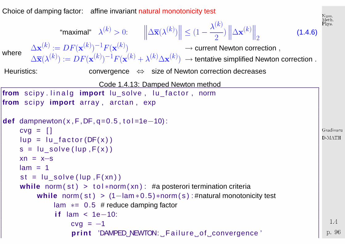
Choice of damping factor: affine invariant natural monotonicity test

“maximal” λ(k) > 0:∥∥∥∆x(λ(k))

∥∥∥ ≤ (1− λ(k)

2)∥∥∥∆x(k)

∥∥∥2

(1.4.6)

where∆x(k) := DF (x(k))−1F (x(k)) → current Newton correction ,

∆x(λ(k)) := DF (x(k))−1F (x(k) + λ(k)∆x(k)) → tentative simplified Newton correction .

Heuristics: convergence ⇔ size of Newton correction decreases

Code 1.4.13: Damped Newton method1 from sc ipy . l i n a l g impo r t lu_so lve , l u _ f a c t o r , norm2 from sc ipy impo r t array , arctan , exp3

4 def dampnewton( x , F ,DF, q=0.5 , t o l =1e−10) :5 cvg = [ ]6 l up = l u _ f a c t o r (DF( x ) )7 s = lu_so lve ( lup , F ( x ) )8 xn = x−s9 lam = 10 s t = lu_so lve ( lup , F ( xn ) )1 w h il e norm ( s t ) > t o l ∗norm ( xn ) : #a posterori termination criteria2 w h il e norm ( s t ) > (1−lam∗0.5)∗norm ( s ) : #natural monotonicity test3 lam ∗= 0.5 # reduce damping factor4 i f lam < 1e−10:5 cvg = −16 p r i n t ’DAMPED NEWTON: F a i l u r e o f convergence ’


Num.Meth.Phys.

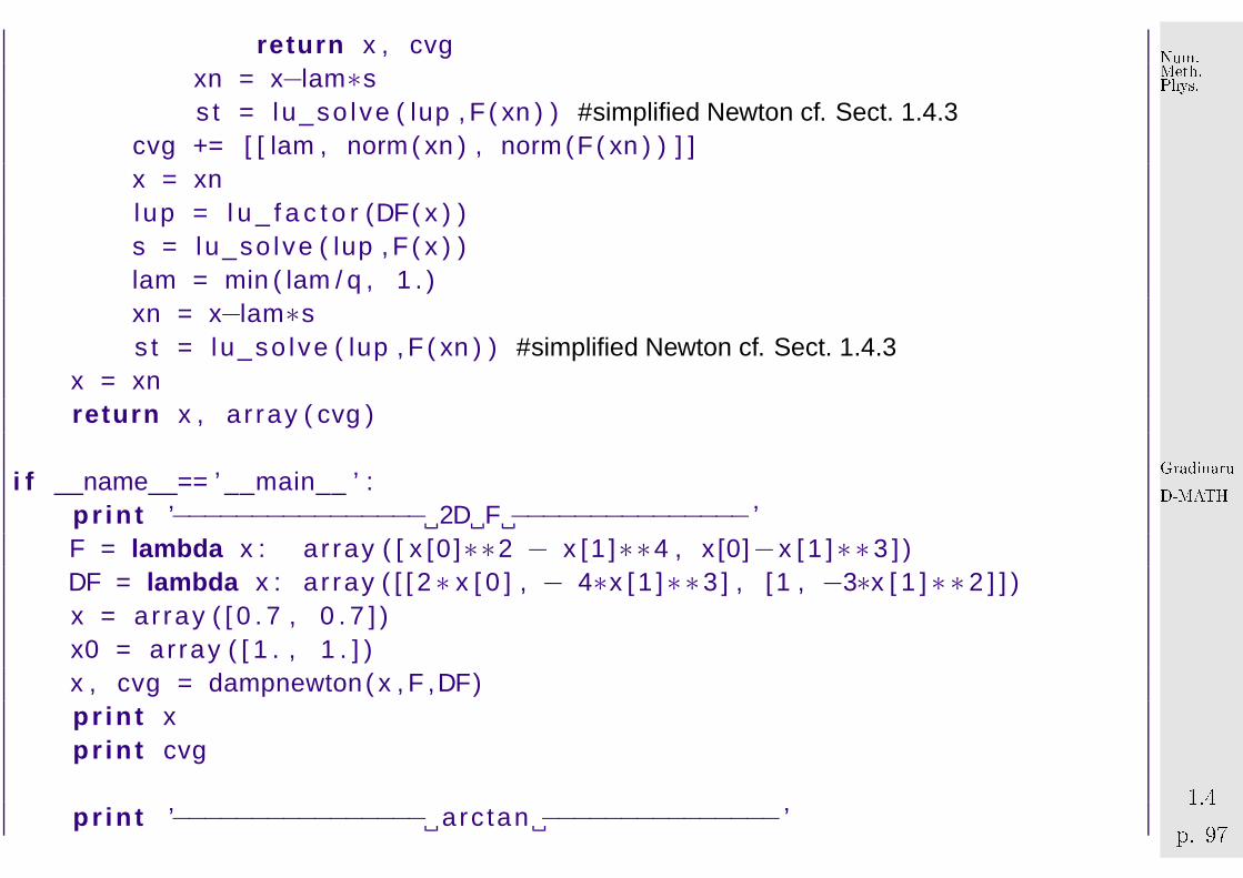
7 r et u r n x , cvg8 xn = x−lam∗s9 s t = lu_so lve ( lup , F ( xn ) ) #simplified Newton cf. Sect. 1.4.30 cvg += [ [ lam , norm ( xn ) , norm (F( xn ) ) ] ]1 x = xn2 l up = l u _ f a c t o r (DF( x ) )3 s = lu_so lve ( lup , F ( x ) )4 lam = min ( lam / q , 1 . )5 xn = x−lam∗s6 s t = lu_so lve ( lup , F ( xn ) ) #simplified Newton cf. Sect. 1.4.37 x = xn8 r et u r n x , a r ray ( cvg )9

0 i f __name__== ’ __main__ ’ :1 p r i n t ’−−−−−−−−−−−−−−−− 2D F −−−−−−−−−−−−−−− ’2 F = lambda x : a r ray ( [ x [0 ]∗∗2 − x [1 ]∗∗4 , x [0]−x [ 1 ]∗∗3 ] )3 DF = lambda x : a r ray ( [ [ 2∗ x [ 0 ] , − 4∗x [ 1 ]∗∗3 ] , [ 1 , −3∗x [ 1 ] ∗ ∗ 2 ] ] )4 x = ar ray ( [ 0 . 7 , 0 . 7 ] )5 x0 = ar ray ( [ 1 . , 1 . ] )6 x , cvg = dampnewton( x , F ,DF)7 p r i n t x8 p r i n t cvg9

0 p r i n t ’−−−−−−−−−−−−−−−− arc tan −−−−−−−−−−−−−−− ’


Num.Meth.Phys.

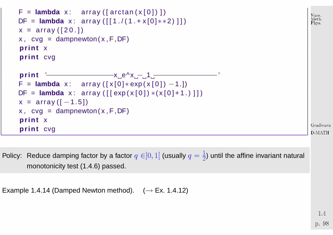
1 F = lambda x : a r ray ( [ a rc tan ( x [ 0 ] ) ] )2 DF = lambda x : a r ray ( [ [ 1 . / ( 1 . + x [0 ]∗∗2 ) ] ] )3 x = ar ray ( [ 2 0 . ] )4 x , cvg = dampnewton( x , F ,DF)5 p r i n t x6 p r i n t cvg7

8 p r i n t ’−−−−−−−−−−−−−−−−x e^x − 1 −−−−−−−−−−−−−−− ’9 F = lambda x : a r ray ( [ x [ 0 ]∗ exp ( x [ 0 ] ) −1.])0 DF = lambda x : a r ray ( [ [ exp ( x [ 0 ] ) ∗( x [ 0 ] + 1 . ) ] ] )1 x = ar ray ( [−1 .5 ] )2 x , cvg = dampnewton( x , F ,DF)3 p r i n t x4 p r i n t cvg

Policy: Reduce damping factor by a factor q ∈]0, 1[ (usually q = 12) until the affine invariant natural

monotonicity test (1.4.6) passed.

Example 1.4.14 (Damped Newton method). (→ Ex. 1.4.12)


Num.Meth.Phys.

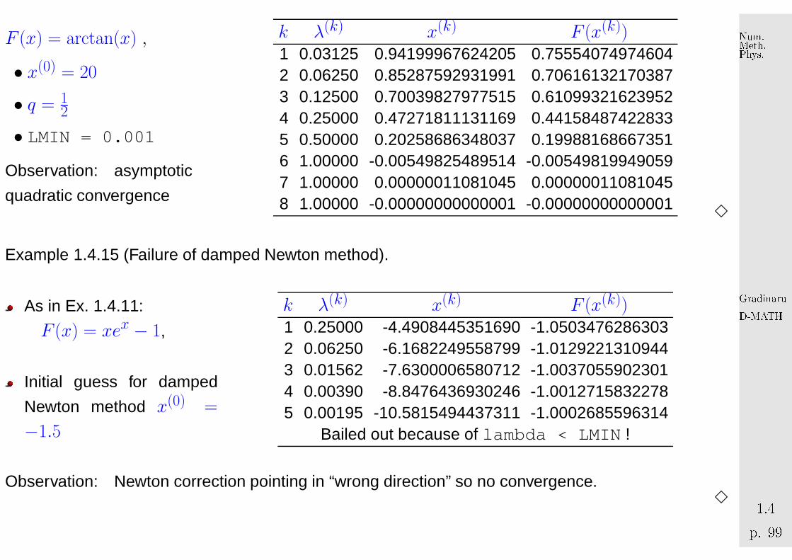
F (x) = arctan(x) ,

• x(0) = 20

• q = 12

• LMIN = 0.001

Observation: asymptotic

quadratic convergence

k λ(k) x(k) F (x(k))1 0.03125 0.94199967624205 0.755540749746042 0.06250 0.85287592931991 0.706161321703873 0.12500 0.70039827977515 0.610993216239524 0.25000 0.47271811131169 0.441584874228335 0.50000 0.20258686348037 0.199881686673516 1.00000 -0.00549825489514 -0.005498199490597 1.00000 0.00000011081045 0.000000110810458 1.00000 -0.00000000000001 -0.00000000000001

3

Example 1.4.15 (Failure of damped Newton method).

As in Ex. 1.4.11:

F (x) = xex − 1,

Initial guess for damped

Newton method x(0) =

−1.5

k λ(k) x(k) F (x(k))1 0.25000 -4.4908445351690 -1.05034762863032 0.06250 -6.1682249558799 -1.01292213109443 0.01562 -7.6300006580712 -1.00370559023014 0.00390 -8.8476436930246 -1.00127158322785 0.00195 -10.5815494437311 -1.0002685596314

Bailed out because of lambda < LMIN !

Observation: Newton correction pointing in “wrong direction” so no convergence.3


Num.Meth.Phys.

1.4.5 Quasi-Newton Method

What to do when DF (x) is not available and numerical differentiation (see remark 1.4.6) is too

expensive?

Idea: in one dimension (n = 1) apply the secant method (1.3.4) of section 1.3.2.3

F ′(x(k)) ≈ F (x(k))− F (x(k−1))

x(k) − x(k−1)"difference quotient" (1.4.7)

already computed ! → cheapGeneralisation for n > 1 ?

Idea: rewrite (1.4.7) as a secant condition for the approximation Jk ≈ DF (x(k)),

x(k) =̂ iterate:

Jk(x(k) − x(k−1)) = F (x(k))− F (x(k−1)) . (1.4.8)

BUT: many matrices Jk fulfill (1.4.8)

Hence: we need more conditions for Jk ∈ Rn,n


Num.Meth.Phys.

Idea: get Jk by a modification of Jk−1

Broyden conditions: Jkz = Jk−1z ∀z: z ⊥ (x(k) − x(k−1)) . (1.4.9)

i.e.: Jk := Jk−1 +F (x(k))(x(k)−x(k−1))T∥∥∥x(k)−x(k−1)

∥∥∥2

2

(1.4.10)

Broydens Quasi-Newton Method for solving F (x) = 0:

x(k+1) := x(k) + ∆x(k), ∆x(k) := −J−1k F (x(k)) , Jk+1 := Jk +

F (x(k+1))(∆x(k))T∥∥∥∆x(k)

∥∥∥2

2(1.4.11)

Initialize J0 e.g. with the exact Jacobi matrix DF (x(0)).

Remark 1.4.16 (Minimal property of Broydens rank 1 modification).

Let J ∈ Rn,n fulfill (1.4.8)

and Jk, x(k) from (1.4.11)then (I− J−1

k J)(x(k+1) − x(k)) = −J−1k F (x(k+1))


Num.Meth.Phys.

and hence

∥∥∥I− J−1k Jk+1

∥∥∥2

=

∥∥∥∥∥∥∥

−J−1k F (x(k+1))∆x(k)

∥∥∥∆x(k)∥∥∥

2

2

∥∥∥∥∥∥∥2

=

∥∥∥∥∥∥∥(I− J−1

k J)∆x(k)(∆x(k))T∥∥∥∆x(k)

∥∥∥2

2

∥∥∥∥∥∥∥2

≤∥∥∥I− J−1

k J

∥∥∥2.

In conlcusion,

(1.4.10) gives the ‖·‖2-minimal relative correction of Jk−1, such that the secant condition (1.4.8)

holds.△ GradinaruD-MATH


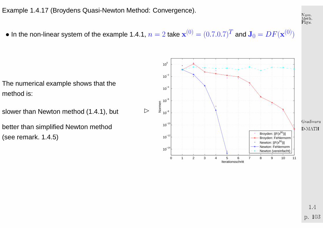
Example 1.4.17 (Broydens Quasi-Newton Method: Convergence).

• In the non-linear system of the example 1.4.1, n = 2 take x(0) = (0.7.0.7)T and J0 = DF (x(0))

The numerical example shows that the

method is:

slower than Newton method (1.4.1), but

better than simplified Newton method

(see remark. 1.4.5)

�

0 1 2 3 4 5 6 7 8 9 10 11

10−14

10−12

10−10

10−8

10−6

10−4

10−2

100

IterationsschrittN

orm

en

Broyden: ||F(x(k))||Broyden: FehlernormNewton: ||F(x(k))||Newton: FehlernormNewton (vereinfacht)


Num.Meth.Phys.

1 2 3 4 5 6 7 8 9 10 11

10−10

10−8

10−6

10−4

10−2

100

Feh

lern

orm

Iterationsschritt1 2 3 4 5 6 7 8 9 10 11

10−2

10−1

100

101

Kon

verg

enzm

onito

r

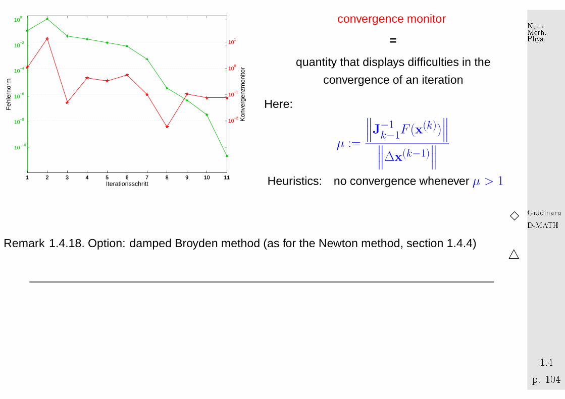
convergence monitor

=

quantity that displays difficulties in the

convergence of an iteration

Here:

µ :=

∥∥∥J−1k−1F (x(k))

∥∥∥∥∥∥∆x(k−1)

∥∥∥Heuristics: no convergence whenever µ > 1

3

Remark 1.4.18. Option: damped Broyden method (as for the Newton method, section 1.4.4)△


Num.Meth.Phys.

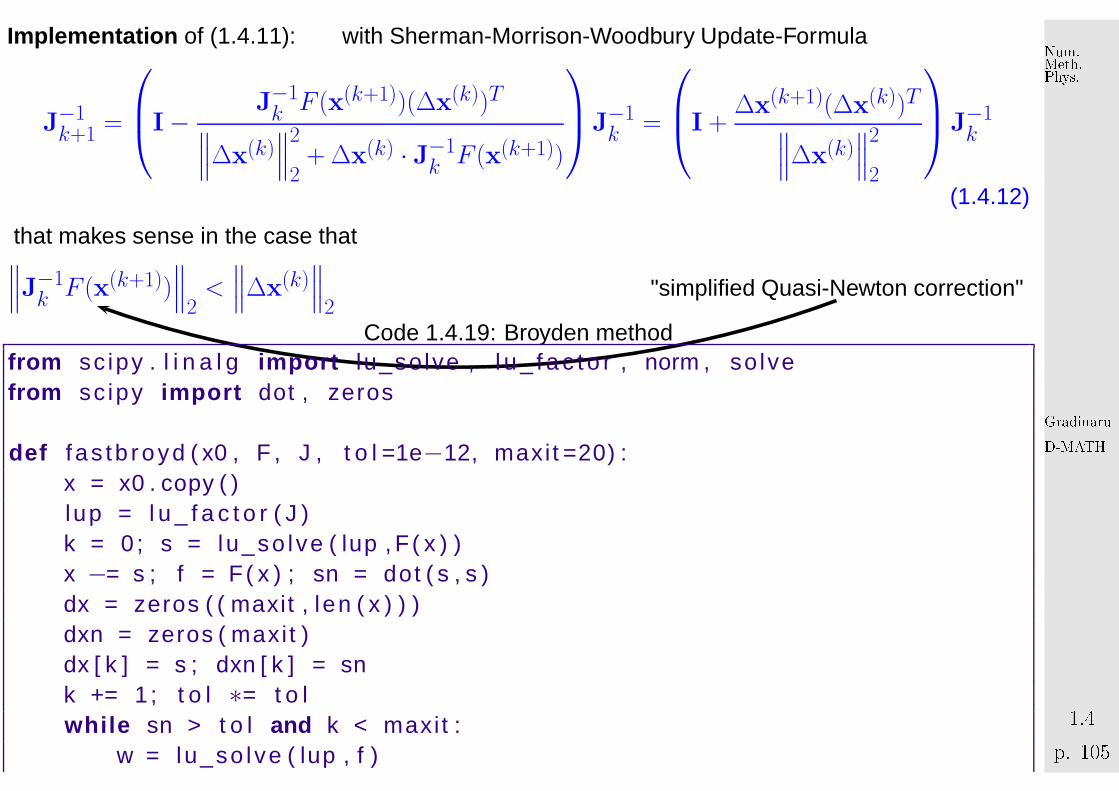
Implementation of (1.4.11): with Sherman-Morrison-Woodbury Update-Formula

J−1k+1 =

I−

J−1k F (x(k+1))(∆x(k))T

∥∥∥∆x(k)∥∥∥

2

2+ ∆x(k) · J−1

k F (x(k+1))

J−1

k =

I +

∆x(k+1)(∆x(k))T∥∥∥∆x(k)

∥∥∥2

2

J−1

k

(1.4.12)

that makes sense in the case that∥∥∥J−1

k F (x(k+1))∥∥∥

2<∥∥∥∆x(k)

∥∥∥2

"simplified Quasi-Newton correction"

Code 1.4.19: Broyden method1 from sc ipy . l i n a l g impo r t lu_so lve , l u _ f a c t o r , norm , so lve2 from sc ipy impo r t dot , zeros3

4 def f as tb royd ( x0 , F , J , t o l =1e−12, maxi t =20) :5 x = x0 . copy ( )6 l up = l u _ f a c t o r ( J )7 k = 0 ; s = lu_so lve ( lup , F ( x ) )8 x −= s ; f = F( x ) ; sn = dot ( s , s )9 dx = zeros ( ( maxit , len ( x ) ) )0 dxn = zeros ( maxi t )1 dx [ k ] = s ; dxn [ k ] = sn2 k += 1 ; t o l ∗= t o l3 w h il e sn > t o l and k < maxit :4 w = lu_so lve ( lup , f )


Num.Meth.Phys.

5 f o r r i n xrange (1 , k ) :6 w += dx [ r ]∗ ( dot ( dx [ r−1] ,w) ) / dxn [ r−1]7 z = dot ( s ,w)8 s = (1+z / ( sn−z ) )∗w9 sn = dot ( s , s )0 dx [ k ] = s ; dxn [ k ] = sn1 x −= s ; f = F( x ) ; k+=12

3 r et u r n x , k

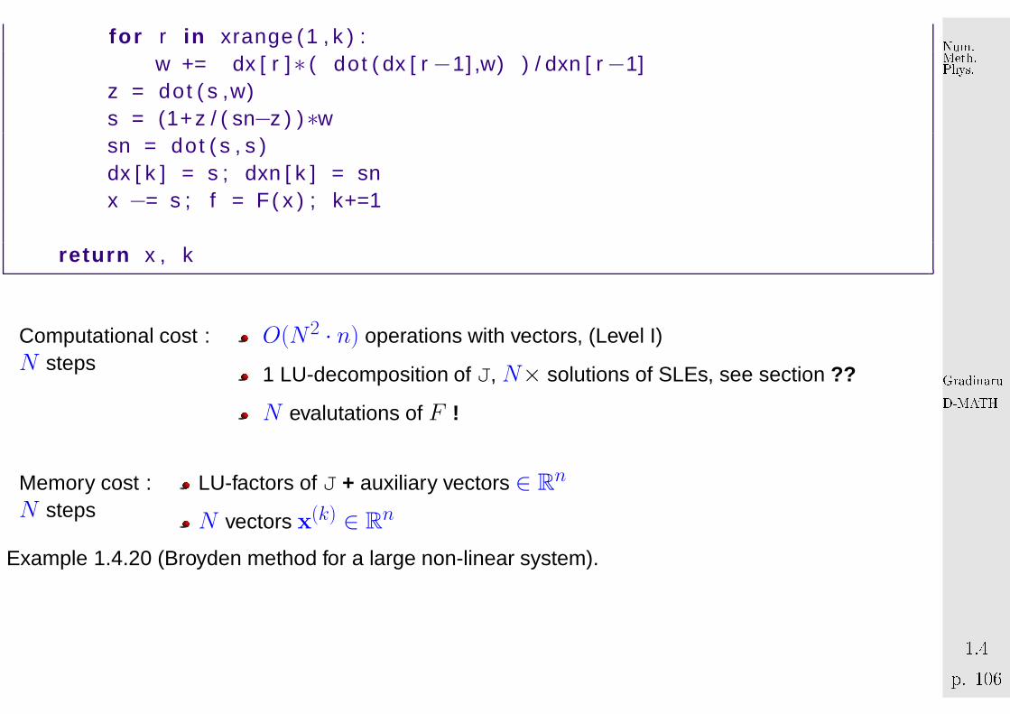
Computational costN steps

: O(N2 · n) operations with vectors, (Level I)

1 LU-decomposition of J, N× solutions of SLEs, see section ??

N evalutations of F !

Memory costN steps

: LU-factors of J + auxiliary vectors ∈ Rn

N vectors x(k) ∈ Rn

Example 1.4.20 (Broyden method for a large non-linear system).


Num.Meth.Phys.

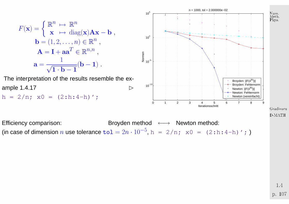
F (x) =

{Rn 7→ R

n

x 7→ diag(x)Ax− b ,

b = (1, 2, . . . , n) ∈ Rn ,

A = I + aaT ∈ Rn,n ,

a =1√

1 · b− 1(b− 1) .

The interpretation of the results resemble the ex-

ample 1.4.17 �

h = 2/n; x0 = (2:h:4-h)’;0 1 2 3 4 5 6 7 8 9

10−10

10−5

100

105

n = 1000, tol = 2.000000e−02

Iterationsschritt

Nor

men

Broyden: ||F(x(k))||Broyden: FehlernormNewton: ||F(x(k))||Newton: FehlernormNewton (vereinfacht)

Efficiency comparison: Broyden method ←→ Newton method:

(in case of dimension n use tolerance tol = 2n · 10−5, h = 2/n; x0 = (2:h:4-h)’; )


Num.Meth.Phys.

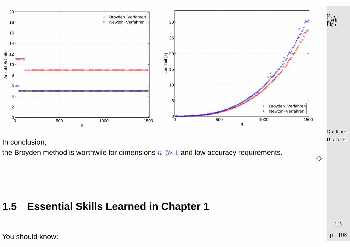
0 500 1000 15000

2

4

6

8

10

12

14

16

18

20

n

Anz

ahl S

chrit

te

Broyden−VerfahrenNewton−Verfahren

0 500 1000 15000

5

10

15

20

25

30

n

Lauf

zeit

[s]

Broyden−VerfahrenNewton−Verfahren

In conclusion,the Broyden method is worthwile for dimensions n≫ 1 and low accuracy requirements.

3

1.5 Essential Skill s Learned in Chapter 1

You should know:


Num.Meth.Phys.

• what is a linear convergent iteration, its rate and dependence of the choice of the norm

• what is the the order of convergence and how to recognize it from plots or from error data

• possible termination criteria and their risks

• how to use fixed-point iterations; convergence criteria

• bisection-method: pros and contras

• Newton-iteration: pros and contras

• the idea behind multi-point methods and an example

• how to use the Newton-method in several dimensions and how to reduce its computational effort

(simplified Newton, quasi-Newton, Broyden method) GradinaruD-MATHp. 1091.5

Num.Meth.Phys.

1 iterative methods for non-linear systems of equations

Documents