iterative methods for linear systems of equations - tu...
TRANSCRIPT

1
PhD-course DTU Informatics, Graduate School ITMANDelft University of Technology
Iterative Methods for LinearSystems of EquationsBasic Iterative Methods
ITMAN PhD-course, DTU, 20-10-08 till 24-10-08
Martin van Gijzen

2
PhD-course DTU Informatics, Graduate School ITMAN
Program day 1
• Overview of the course
• Useful references
• Introduction to iterative methods
• Some general concepts
• Basic iterative methods
• One-step projection methods

3
PhD-course DTU Informatics, Graduate School ITMAN
Goals of the course
• Explain basic ideas;
• Show how these ideas translate into algorithms;
• Give overview of modern iterative methods.
At the end of the course you will
• be able to understand the differences and similarities
between the many iterative methods;
• and you will be able to select a suitable method for your
problem.

4
PhD-course DTU Informatics, Graduate School ITMAN
Daily schedule (tentative)
9.00 - 11.00 Lecture, new theory
11.00 - 12.00 Theoretical exercises
12.00 - 13.30 Lunch
13.30 - 14.00 Introduction to an application
14.00 - 16.00 MATLAB-assignment

5
PhD-course DTU Informatics, Graduate School ITMAN
Topics per day• Day 1: Basic iterative methods
• Day 2: Projection methods (1)
Krylov methods for symmetric systems: CG, MINRES,
methods for the normal equations
• Day 3: Projection methods (2)
Krylov methods for nonsymmetric systems:
GMRES-type methods
• Day 4: Projection methods (3)
Krylov methods for nonsymmetric systems: BiCG-type
methods
• Day 5: Preconditioning techniques

6
PhD-course DTU Informatics, Graduate School ITMAN
Recommended literature• Gene H. Golub and Charles F. Van Loan. Matrix
Computations. 3rd ed. The Johns Hopkins UniversityPress, Baltimore, 1996.
• Richard Barrett, Michael Berry, Tony Chan, JamesDemmel, June Donato, Jack Dongarra, Victor Eijkhout,Roidan Pozo, Charles Romine, Henk van der Vorst.Templates for the Solution of Linear Systems: BuildingBlocks for Iterative Methods. 2nd edition, SIAM, 1994.
• Henk van der Vorst, Iterative Krylov methods for largelinear systems. Cambridge press, 2003
• Yousef Saad, Iterative Methods for Sparse LinearSystems. 2nd ed. SIAM, 2003

7
PhD-course DTU Informatics, Graduate School ITMAN
Useful webpages• http://www.netlib.org/: a wealth of information on a.o.
numerical software, e.g.
• LAPACK, BLAS: dense linear algebra
• NETSOLVE: grid computing
• TEMPLATES: the book plus software
• MATRIX MARKET: matrices
• http://www.math.uu.nl/people/vorst/: manuscript of the book,
software
• http://www-users.cs.umn.edu/ saad/: first edition of the
book, software
• http://www2.imm.dtu.dk/ pch/: interesting links, software

8
PhD-course DTU Informatics, Graduate School ITMAN
Introduction to iterative methods
Many applications give rise to (non)linear systems of equations.
Typically the system matrices are
• Large, 108 unknowns are not exceptional anymore;
• Sparse, only a fraction of the entries of the matrix is
nonzero;
• Structured, the matrix often has a symmetric pattern and is
banded.
Moreover, the matrix can have special numerical properties, e.g it
may be symmetric, Toeplitz, or the eigenvalues may all be in the
right-half plane.
9
PhD-course DTU Informatics, Graduate School ITMAN
An application: ocean circulation (1)
Physical model: balance between
• Wind force
• Coriolis force
• Bottom friction.
10
PhD-course DTU Informatics, Graduate School ITMAN
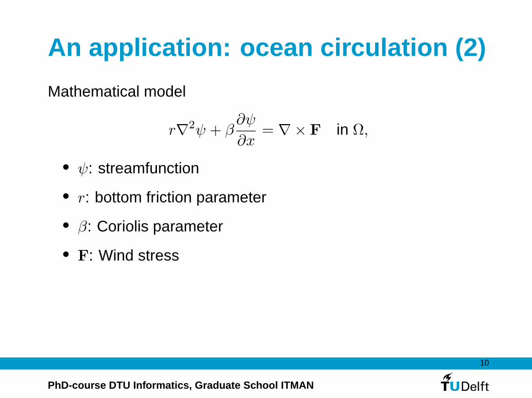
An application: ocean circulation (2)
Mathematical model
r∇2ψ + β∂ψ
∂x= ∇× F in Ω,
• ψ: streamfunction
• r: bottom friction parameter
• β: Coriolis parameter
• F: Wind stress

11
PhD-course DTU Informatics, Graduate School ITMAN
An application: ocean circulation (3)
Numerical model: discretisation with FEM
12
PhD-course DTU Informatics, Graduate School ITMAN
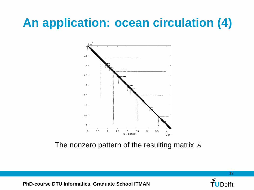
An application: ocean circulation (4)
0 0.5 1 1.5 2 2.5 3 3.5 4
x 104
0
0.5
1
1.5
2
2.5
3
3.5
4
x 104
nz = 294785
The nonzero pattern of the resulting matrix A

13
PhD-course DTU Informatics, Graduate School ITMAN
Why iterative methods?
Direct methods: A = LU .
Due to fill-in L and U can not be stored for realistic problems.
This is in particular true for three dimensional (3D) problems.
Model problem Direct Iterative
Computational O(np) O(np)
costs p ≈ 2.0 for 2D p ≈ 1.4 for 2D
p ≈ 2.3 for 3D p ≈ 1.2 for 3D
Memory O(np) O(n)
requirements p ≈ 1.5 for 2D
p ≈ 1.7 for 3D

14
PhD-course DTU Informatics, Graduate School ITMAN
Iterative versus direct
For many problems, it is not clear which method is best:
• Direct methods are robust
• O(np) can have a very large constant for iterative methods
• Often a combination can be used, e.g. in domain
decomposition or iterative refinement
15
PhD-course DTU Informatics, Graduate School ITMAN
Does the best iterative method exist?
If no further restrictions: no
For certain classes: yes
Success of any iterative method depends on:
• Properties of A
(Size, sparsity structure, symmetry, ...)
• Computer architecture
(scalar, parallel, memory organisation, ...)
• Memory space available
• Accuracy required

16
PhD-course DTU Informatics, Graduate School ITMAN
Some general concepts
Iterative methods construct successive approximations xk to the
solution of the linear systems Ax = b. Here k is the iteration
number, and the approximation xk is also called the iterate. The
vector rk = b−Axk is the residual.
The iterative methods are composed of only a few different basic
operations:
• Products with the matrix A
• Vector operations (updates and inner product operations)
• Preconditioning operations

17
PhD-course DTU Informatics, Graduate School ITMAN
PreconditioningUsually iterative methods are applied not to the original system
Ax = b
but to the preconditioned system
M−1Ax = M−1b
where the preconditioner is chosen such that:
• Preconditioning operations (operations with M−1) are
cheap;
• The iterative method converges much faster for the
preconditioned system.
Preconditioners will be discussed in more detail on day 5.

18
PhD-course DTU Informatics, Graduate School ITMAN
Basic iterative methods
The first iterative methods we will discuss are the basiciterative methods. Basic iterative methods only useinformation of the previous iteration.
Until the 70’s they were quite popular. Some are still usedbut as preconditioners in combination with an accelerationtechnique. They also still play a role in multigrid techniqueswhere they are used as smoothers. Multigrid methods arediscussed on day 5 of this course.

19
PhD-course DTU Informatics, Graduate School ITMAN
Basic iterative methods (2)
Basic iterative methods are usually constructed using a splitting
of A:
A = M −R.
Successive approximations are then computed using the
iterative process
Mxk+1 = Rxk + b
which is equivalent too
xk+1 = xk +M−1(b−Axk)
The vector rk = b−Axk is called the residual, and the matrix M
is a preconditioner. The next few slides we look at M = I.
20
PhD-course DTU Informatics, Graduate School ITMAN
Richardson’s method
The choice M = I, R = I −A gives Richardson’s method, which
is the most simple iterative method possible.
The iterative process becomes
xk+1 = xk + (b−Axk) = b+ (I −A)xk

21
PhD-course DTU Informatics, Graduate School ITMAN
Richardson’s method (2)
This process yields the following iterates:
Initial guess x0 = 0
x1 = b
x2 = b+ (I −A)x(1) = b+ (I −A)b
x3 = b+ (I −A)x(2) = b+ (I −A)b+ (I −A)2b
Repeating this gives
xk+1 =k∑
i=0
(I −A)ib

22
PhD-course DTU Informatics, Graduate School ITMAN
Richardson’s method (3)
So Richardson’s method generates the series expansion for 11−z
with z = I −A. If this series converges we have
∞∑
i=0
(I −A)i = A−1
The series expansion for 11−z
converges if |z| < 1. If A is
diagonalizable then the series∑∞
i=0(I −A)i converges if
|1 − λ| < 1
with λ any eigenvalue of A. For λ real this means that
0 < λ < 2
23
PhD-course DTU Informatics, Graduate School ITMAN
Richardson’s method (4)
In order to increase the radius of convergence and to speed up
the convergence, one can introduce a parameter α:
xk+1 = xk + α(b−Axk) = αb+ (I − αA)xk
It is easy to verify that the optimal α which gives fastest
convergence is given by
αopt =2
λmax + λmin
.

24
PhD-course DTU Informatics, Graduate School ITMAN
Richardson’s method (5)
Before, we assumed for the initial guess x0 = 0.
Starting with another initial guess x0 only
means that we have to solve a shifted system
A(y + x0) = b⇔ Ay = b−Ax0 = r0
So the results obtained before remain valid, irrespective of the
initial guess.

25
PhD-course DTU Informatics, Graduate School ITMAN
Richardson’s method (6)
We want to stop once the error ‖xk − x‖ < ǫ, with ǫ some
prescribed tolerance. Unfortunately we do not know x, so this
criterion does not work in practice.
Alternatives are:
• ‖rk‖ = ‖b−Axk‖ = ‖Ax−Axk‖ < ǫ
Disadvantage: criterion not scaling invariant
• ‖rk‖‖r0‖
< ǫ
Disadvantage: good initial guess does not reduce the
number of iterations
• ‖rk‖‖b‖ < ǫ
Seems best
26
PhD-course DTU Informatics, Graduate School ITMAN
Convergence theory
To investigate the convergence of Basic Iterative Methods in
general, we look again at the formula
Mxk+1 = Rxk + b.
Remember that A = M −R. If we subtract Mx = Rx+ b from
this equation we get a recursion for the error e = xk − x:
Mek+1 = Rek
27
PhD-course DTU Informatics, Graduate School ITMAN
Convergence theory (2)
We can also write this as
ek+1 = M−1Rek
This is a power iteration and hence the error will ultimately point
in the direction of the largest eigenvector of M−1R. The rate of
convergence is determined by the spectral radius ρ(M−1R) of
M−1R:
ρ(M−1R) = |λmax(M−1R)| .
For convergence we must have that
ρ(M−1R) < 1 .
28
PhD-course DTU Informatics, Graduate School ITMAN
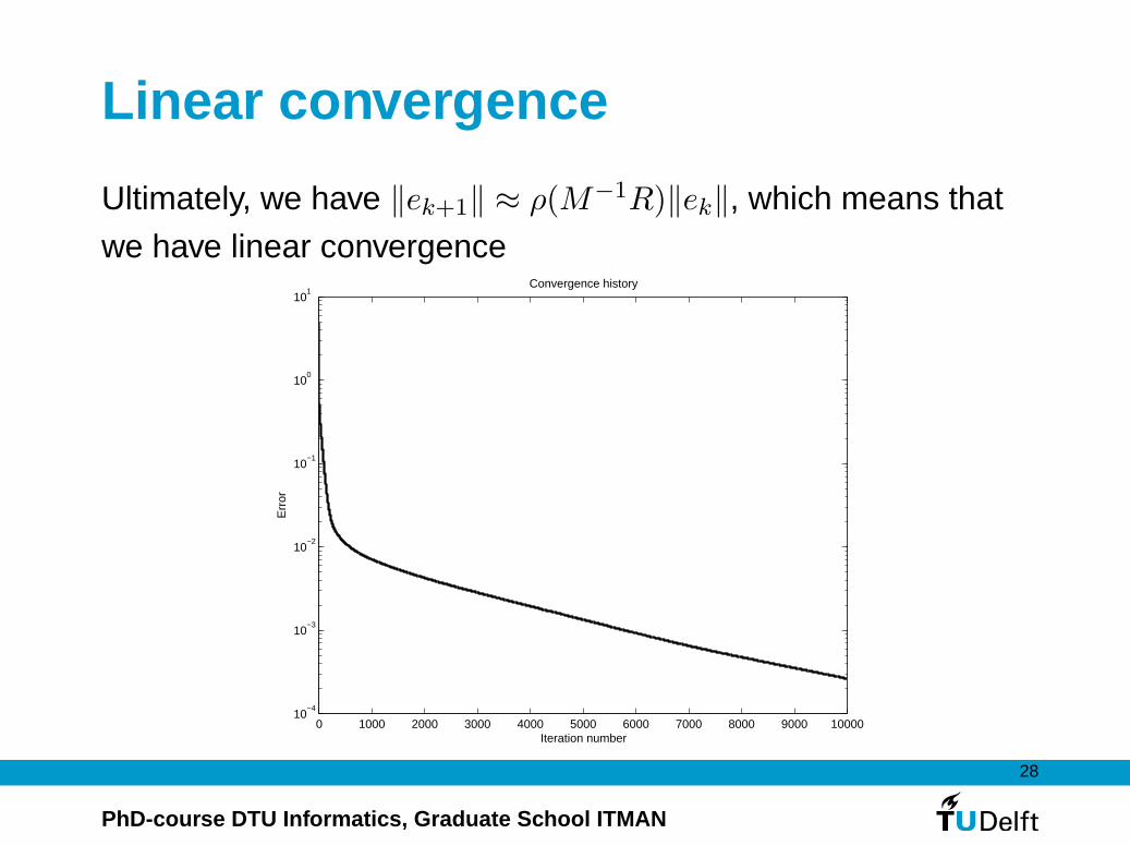
Linear convergence
Ultimately, we have ‖ek+1‖ ≈ ρ(M−1R)‖ek‖, which means that
we have linear convergence
0 1000 2000 3000 4000 5000 6000 7000 8000 9000 1000010
−4
10−3
10−2
10−1
100
101
Convergence history
Iteration number
Err
or

29
PhD-course DTU Informatics, Graduate School ITMAN
Classical Basic Iterative Methods
We will now briefly discuss the three best known basic iterative
methods
• Jacobi’s method
• The method of Gauss-Seidel
• Successive overrelaxation
These methods can be seen as Richardson’s method applied to
the preconditioned system
M−1Ax = M−1b .
30
PhD-course DTU Informatics, Graduate School ITMAN
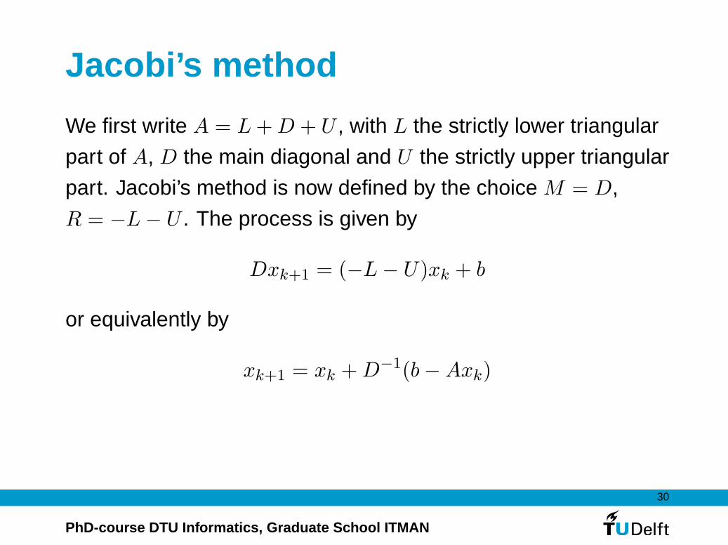
Jacobi’s method
We first write A = L+D + U , with L the strictly lower triangular
part of A, D the main diagonal and U the strictly upper triangular
part. Jacobi’s method is now defined by the choice M = D,
R = −L− U . The process is given by
Dxk+1 = (−L− U)xk + b
or equivalently by
xk+1 = xk +D−1(b−Axk)

31
PhD-course DTU Informatics, Graduate School ITMAN
The Gauss-Seidel method
We write again A = L+D + U . The Gauss-Seidel method is
now defined by the choice M = L+D, R = −U . The process is
given by
(L+D)xk+1 = −Uxk + b
or equivalently by
xk+1 = xk + (L+D)−1(b−Axk)
32
PhD-course DTU Informatics, Graduate School ITMAN
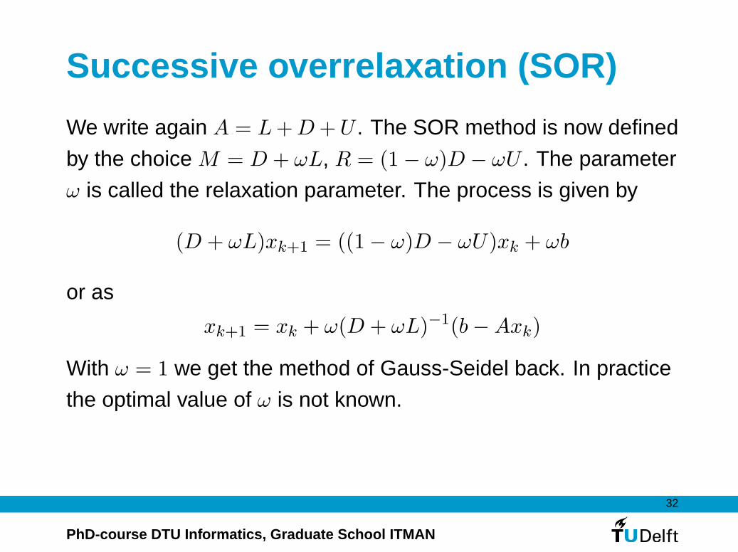
Successive overrelaxation (SOR)
We write again A = L+D+U . The SOR method is now defined
by the choice M = D + ωL, R = (1 − ω)D − ωU . The parameter
ω is called the relaxation parameter. The process is given by
(D + ωL)xk+1 = ((1 − ω)D − ωU)xk + ωb
or as
xk+1 = xk + ω(D + ωL)−1(b−Axk)
With ω = 1 we get the method of Gauss-Seidel back. In practice
the optimal value of ω is not known.
33
PhD-course DTU Informatics, Graduate School ITMAN
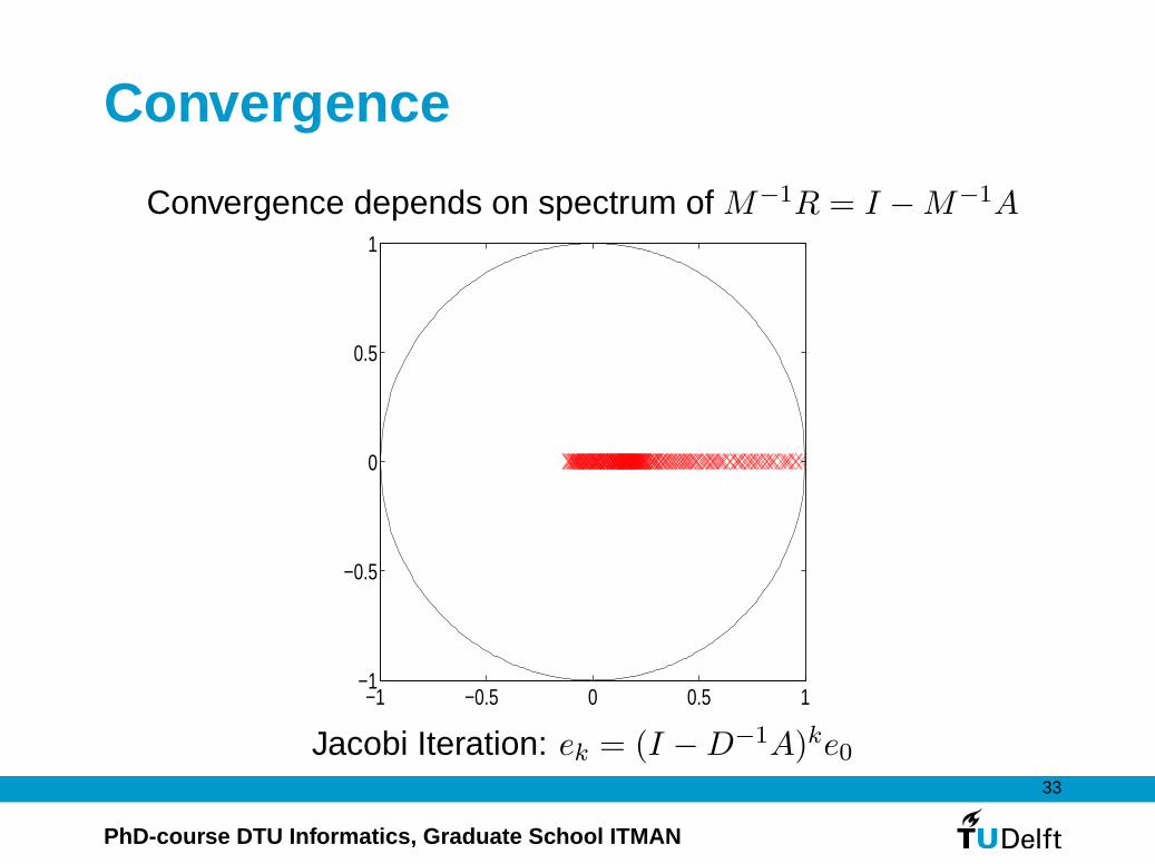
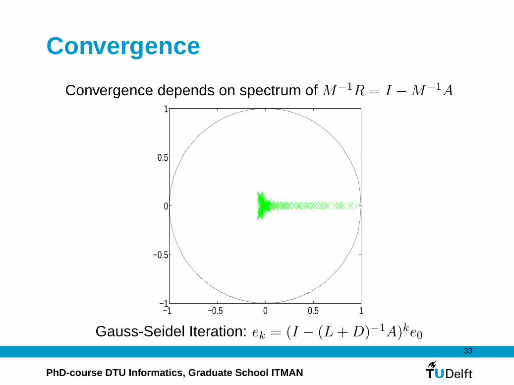
Convergence
Convergence depends on spectrum of M−1R = I −M−1A
−1 −0.5 0 0.5 1−1
−0.5
0
0.5
1
Jacobi Iteration: ek = (I −D−1A)ke0
33
PhD-course DTU Informatics, Graduate School ITMAN
Convergence
Convergence depends on spectrum of M−1R = I −M−1A
−1 −0.5 0 0.5 1−1
−0.5
0
0.5
1
Gauss-Seidel Iteration: ek = (I − (L+D)−1A)ke0
34
PhD-course DTU Informatics, Graduate School ITMAN
One-step projection methods
The convergence of Richardson’s method is not guaranteed and
if the method converges, convergence is often very slow.
We now introduce two methods that are guaranteed to converge
for wide classes of matrices. The two methods take special
linear combinations of the vectors rk and Ark to construct a new
iterate xk+1 that satisfies a local optimality property.

35
PhD-course DTU Informatics, Graduate School ITMAN
Steepest descent
Let A be symmetric positive definite. Define the function
f(xk) = ‖xk − x‖2A = (xk − x)TA(xk − x)
Let xk+1 = xk + αkrk Then the choice
αk =rTk rk
rTk Ark
minimizes f(xk+1).

36
PhD-course DTU Informatics, Graduate School ITMAN
Minimal residual
Let A be general square. Define the function
g(xk) = ‖b−Axk‖22 = rT
k rk
Let xk+1 = xk + αkrk Then the choice
αk =rTk Ark
rTk A
TArk
minimizes g(xk+1).

37
PhD-course DTU Informatics, Graduate School ITMAN
Orthogonality properties
The optimality properties of the steepest descent method and
the minimal residual method are equivalent with the following
orthogonality properties:
For steepest descent
αk =rTk rk
rTk Ark
⇒ rk+1 ⊥ rk
For the minimal residual method
αk =rTk Ark
rTk A
TArk⇒ rk+1 ⊥ Ark .
38
PhD-course DTU Informatics, Graduate School ITMAN
Summary
Today we introduced Richardson’s method and three
preconditioned variants: the methods of Jacobi and
Gauss-Seidel and the Successive Overrelaxation Technique.
We saw that the convergence of Richardson’s method can be
related to the convergence of the series 11−z
= 1 + z + z2 · · · . If
the method converges, convergence is linear, and often slow.
The question is whether there are better, faster ways to
approximate A−1 using a polynomial expansion.
Tomorrow we will investigate how we can construct such
methods.