A Local Discontinuous Galerkin Method for KdV Type Equations1

Jue Yan2 and Chi-Wang Shu3

Division of Applied Mathematics

Brown University

Providence, Rhode Island 02912

ABSTRACT

In this paper we develop a local discontinuous Galerkin method for solving KdV type

equations containing third derivative terms in one and two space dimensions. The method

is based on the framework of the discontinuous Galerkin method for conservation laws and

the local discontinuous Galerkin method for viscous equations containing second derivatives,

however the guiding principle for inter-cell uxes and nonlinear stability is new. We prove

L2 stability and a cell entropy inequality for the square entropy for a class of nonlinear

PDEs of this type both in one and multiple spatial dimensions, and give an error estimate

for the linear cases in the one dimensional case. The stability result holds in the limit case

when the coeÆcients to the third derivative terms vanish, hence the method is especially

suitable for problems which are \convection dominate", i.e. those with small second and

third derivative terms. Numerical examples are shown to illustrate the capability of this

method. The method has the usual advantage of local discontinuous Galerkin methods,

namely it is extremely local and hence eÆcient for parallel implementations and easy for h-p

adaptivity.

Key Words: Discontinuous Galerkin method, KdV equation, stability, error estimate.

AMS(MOS) subject classi�cation: 65M60,35Q53.

1Research supported by ARO grant DAAD19-00-1-0405, NSF grants DMS-9804985 and ECS-9906606,

NASA Langley grant NCC1-01035 and Contract NAS1-97046 while the second author was in residence at

ICASE, NASA Langley Research Center, Hampton, VA 23681-2199, and AFOSR grant F49620-99-1-0077.2E-mail: yjue@cfm.brown.edu3E-mail: shu@cfm.brown.edu

1

1 Introduction

In this paper we develop a local discontinuous Galerkin method for solving KdV type equa-

tions containing third derivative terms in one and multiple spatial dimensions. An example

of such PDEs is the original KdV equation [18]

ut + (�u+ �u2)x + �uxxx = 0; (1.1)

where �, � and � are constants. Our scheme can be designed and proven stable for more

general nonlinearities, namely

ut + f(u)x + (r0(u)g(r(u)x)x)x = 0 (1.2)

in one space dimension for arbitrary (smooth) functions f , g and r, and

ut +dX

i=1

fi(u)xi +dX

i=1

r0i(u)

dXj=1

gij(ri(u)xi)xj

!xi

= 0 (1.3)

in multiple spatial dimensions for arbitrary (smooth) functions fi, gij and ri.

KdV type equations describe the propagation of waves in a variety of nonlinear, dispersive

media and appear often in applications. See, e.g. [1]. Various numerical methods have been

proposed and used in practice to solve this type of equations, see, e.g. [4, 5, 17]. However,

in many situations, such as in the quantum hydrodynamic models of semiconductor device

simulations [15] and in the dispersive limit of conservation laws [19], the third derivative

terms might have small or even zero coeÆcients in some parts of the domain. We will call

such cases as \convection dominated". The design of stable, eÆcient and high order methods,

especially those for the \convection dominated" cases, i.e. when the third derivative terms

are small (j�j � 1 in (1.1)), remains a challenge.

The discontinuous Galerkin method is a class of �nite element methods using completely

discontinuous piecewise polynomial space for the numerical solution and the test functions.

One certainly needs to use more degrees of freedom because of the discontinuities at the

element boundaries, however this also gives one a room to design suitable inter-element

2

boundary treatments (the so-called uxes) to obtain highly accurate and stable methods in

many diÆcult situations.

The �rst discontinuous Galerkin method was introduced in 1973 by Reed and Hill [20],

in the framework of neutron transport (steady state linear hyperbolic equations). A major

development of the discontinuous Galerkin method was carried out by Cockburn et al. in a

series of papers [10, 9, 7, 11], in which they established a framework to easily solve nonlinear

time dependent hyperbolic conservation laws (i.e. (1.2) and (1.3) without the third derivative

terms) using explicit, nonlinearly stable high order Runge-Kutta time discretizations [22] and

discontinuous Galerkin discretization in space with exact or approximate Riemann solvers

as interface uxes and TVB (total variation bounded) nonlinear limiters [21] to achieve

non-oscillatory properties for strong shocks.

The discontinuous Galerkin method has found rapid applications in such diverse areas

as aeroacoustics, electro-magnetism, gas dynamics, granular ows, magneto-hydrodynamics,

meteorology, modeling of shallow water, oceanography, oil recovery simulation, semiconduc-

tor device simulation, transport of contaminant in porous media, turbomachinery, turbulent

ows, viscoelastic ows and weather forecasting, among many others. Good references for

the discontinuous Galerkin method and its recent development include the survey paper [8],

other papers in that Springer volume, and the review paper [13].

The original discontinuous Galerkin method was designed to solve �rst order hyperbolic

problems. A simple example to illustrate the essential ideas is the linear transport equation

ut + ux = 0: (1.4)

Let's denote the mesh by Ij =[xj� 1

2

; xj+ 1

2

], for j = 1; :::; N , with the center of the cell denoted

by xj =1

2

�xj� 1

2

+ xj+ 1

2

�and the size of each cell by �xj = xj+ 1

2

� xj� 1

2

. We will denote

�x = maxj �xj . If we multiply (1.4) by an arbitrary test function v(x), integrate over the

interval Ij, and integrate by parts, we getZIj

utvdx�ZIj

uvxdx + u(xj+ 1

2

; t)v(xj+ 1

2

)� u(xj� 1

2

; t)v(xj� 1

2

) = 0: (1.5)

3

This is the starting point for designing the discontinuous Galerkin method. We replace both

the solution u and the test function v by piecewise polynomials of degree at most k. That

is, u; v 2 V�x where

V�x = fv : v is a polynomial of degree at most k for x 2 Ij; j = 1; :::; Ng : (1.6)

With this choice, there is an ambiguity in (1.5) in the last two terms involving the boundary

values at xj� 1

2

, as both the solution u and the test function v are discontinuous exactly

at these boundary points. The idea is to treat these terms by an upwinding mechanism

(information from characteristics), borrowed from successful high resolution �nite volume

schemes. Thus u at the interfaces xj� 1

2

is given by a single valued numerical ux uj� 1

2

= u�j� 1

2

,

determined from upwinding, and v at the interfaces xj� 1

2

are given by the values taken from

inside the cell Ij, namely v�j+ 1

2

and v+j� 1

2

. Notice that we use v� and v+ to denote the left and

right limits of v, respectively, at the interface where v is discontinuous. For more general

nonlinear uxes f(u), the only di�erence is that the single valued ux fj+ 1

2

would be taken

as a monotone ux depending on both u�j+ 1

2

and on u+j+ 1

2

(exact or approximate Riemann

solvers in the system case). The resulting method of the lines ODE is then discretized by the

nonlinearly stable high order Runge-Kutta time discretizations [22]. Nonlinear TVB limiters

[21] may be used if the solution contains strong discontinuities. The schemes thus obtained,

for solving hyperbolic conservation laws ((1.2) and (1.3) without the third derivative terms),

have the following attractive properties:

1. It can be easily designed for any order of accuracy. In fact, the order of accuracy can

be locally determined in each cell, thus allowing for eÆcient p adaptivity.

2. It can be used on arbitrary triangulations, even those with hanging nodes, thus allowing

for eÆcient h adaptivity.

3. It is extremely local in data communications. The evolution of the solution in each

cell needs to communicate only with the immediate neighbors, regardless of the order

of accuracy, thus allowing for eÆcient parallel implementations. See, e.g. [3].

4

4. It has excellent provable nonlinear stability. One can prove a strong L2 stability and

a cell entropy inequality for the square entropy, for the general nonlinear cases, for

any orders of accuracy on arbitrary triangulations in any space dimension, without the

need for nonlinear limiters [16].

In [12] these discontinuous Galerkin methods were generalized to solve convection dif-

fusion problems containing second derivative terms. This was motivated by the successful

numerical experiments of Bassi and Rebay [2] for the compressible Navier-Stokes equations.

The idea can be illustrated with the simple heat equation

ut � uxx = 0 (1.7)

which we rewrite into a �rst order system

ut � qx = 0; q � ux = 0; (1.8)

we can then formally use the same discontinuous Galerkin method for the convection equation

to solve (1.8), resulting in the following scheme: �nd u; q 2 V�x such that, for all test

functions v; w 2 V�x,ZIj

utvdx+

ZIj

qvxdx� qj+ 1

2

v�j+ 1

2

+ qj� 1

2

v+j� 1

2

= 0ZIj

qwdx+

ZIj

uwxdx� uj+ 1

2

w�j+ 1

2

+ uj� 1

2

w+

j� 1

2

= 0: (1.9)

However, there is no longer a upwinding mechanism or characteristics to guide the design of

the uxes uj+ 1

2

and qj+ 1

2

. The crucial part in designing a stable and accurate algorithm (1.9)

is a correct design of these uxes. In [12], criteria are given for these uxes to guarantee

stability, convergence and a sub-optimal error estimate of order k for piecewise polynomials

of degree k. The (most natural) central uxes

uj+ 1

2

=1

2

�u�j+ 1

2

+ u+j+ 1

2

�; qj+ 1

2

=1

2

�q�j+ 1

2

+ q+j+ 1

2

�(1.10)

would satisfy these criteria and give a scheme which is indeed sub-optimal in the order of

accuracy for odd k (i.e. the accuracy is order k rather than the expected order k+1 for odd

5

k). This de�ciency however is easily removed by going to a clever choice of uxes, proposed

in [12]:

uj+ 1

2

= u�j+ 1

2

; qj+ 1

2

= q+j+ 1

2

: (1.11)

i.e. we alternatively take the left and right limits for the uxes in u and q (we could of

course also take the pair u+j+ 1

2

and q�j+ 1

2

as the uxes). Notice that the evaluation of (1.11)

is simpler than that of the central uxes in (1.10), and this easily generalizes to multi space

dimensions on arbitrary triangulations. The accuracy now becomes the optimal order k + 1

for both even and odd k.

The schemes thus designed for the heat equation (1.7), or in fact for the most general multi

dimensional nonlinear convection di�usion equations (nonlinear both in the �rst derivative

convection part and the second derivation di�usion part), retain all the four nice properties

listed above for the method used on convection equations. Moreover, the appearance of the

auxiliary variable q is super�cial: when a local basis is chosen in cell Ij then q is eliminated

and the actual scheme for u takes a form similar to that for convection alone. This is a big

advantage of the scheme over the traditional \mixed methods", and it is the reason that the

scheme is termed local discontinuous Galerkin method in [12]. Even though the auxiliary

variable q can be locally eliminated, it does approximate the derivative of the solution u to

the same order of accuracy, thus matching the advantage of traditional \mixed methods" on

this.

The purpose of this paper is to develop a similar local discontinuous Galerkin (LDG)

method for the KdV like equations (1.1), (1.2) and (1.3) containing third derivative terms.

Our objective is to design the method to retain again all the four nice properties listed above

for the method used on convection and convection-di�usion equations, plus the feature that

the method is local, namely the auxiliary variables introduced to approximate the �rst and

second derivatives of the solution could be locally eliminated.

We will give a \preview" of the method on the simple linear equation

ut + uxxx = 0 (1.12)

6

which we again rewrite into a �rst order system

ut + px = 0; p� qx = 0; q � ux = 0: (1.13)

We can then formally use the same discontinuous Galerkin method for the convection equa-

tion to solve (1.13), resulting in the following scheme: �nd u; p; q 2 V�x such that, for all

test functions v; w; z 2 V�x,ZIj

utvdx�ZIj

pvxdx + pj+ 1

2

v�j+ 1

2

� pj� 1

2

v+j� 1

2

= 0;ZIj

pwdx+

ZIj

qwxdx� qj+ 1

2

w�j+ 1

2

+ qj� 1

2

w+

j� 1

2

= 0; (1.14)ZIj

qzdx +

ZIj

uzxdx� uj+ 1

2

z�j+ 1

2

+ uj� 1

2

z+j� 1

2

= 0:

However, the uxes pj+ 1

2

, qj+ 1

2

and uj+ 1

2

must be designed based on di�erent guiding prin-

ciples than the �rst order convection or second order di�usion cases. The crucial part in

designing a stable and accurate algorithm (1.14) is again a correct design of these uxes. It

turns out that the simple choices

pj+ 1

2

= p+j+ 1

2

; qj+ 1

2

= q+j+ 1

2

; uj+ 1

2

= u�j+ 1

2

; (1.15)

would guarantee stability and convergence, as can be proven later in this paper and also

clearly seen in Table 1.1, which contains numerical L2 and L1 errors and orders of accuracy

for the computed solution u for the method (1.14) with the uxes (1.15) solving the equation

(1.12) with an initial condition u(x; 0) = sin(x) over the interval [0; 2�] and periodic boundary

conditions, at t = 1, using uniform meshes.

We remark that the choice for the uxes (1.15) is not unique. In fact, the crucial part is

to take p and u from opposite sides and to take q from the right. Thus

pj+ 1

2= p�

j+ 1

2

; qj+ 1

2= q+

j+ 1

2

; uj+ 1

2= u+

j+ 1

2

;

would also work.

7

Table 1.1: ut+ uxxx = 0. u(x; 0) = sin(x). Periodic boundary conditions. L2 and L1 errors.Uniform meshes with N cells. LDG methods with k = 0; 1; 2; 3. t = 1.

k N=10 N=20 N=40 N=80error error order error order error order

0 L2 2.2534E-01 1.2042E-01 0.91 6.2185E-02 0.95 3.1582E-02 0.98L1 4.3137E-01 2.1977E-01 0.97 1.1082E-01 0.98 5.5376E-02 1.00

1 L2 1.7150E-02 4.2865E-03 2.00 1.0716E-03 2.00 2.6792E-04 1.99L1 5.8467E-02 1.5757E-02 1.89 4.0487E-03 1.96 1.0210E-03 1.99

2 L2 8.5803E-04 1.0823E-04 2.98 1.3559E-05 2.99 1.6958E-06 3.00L1 4.0673E-03 5.1029E-04 2.99 6.4490E-05 2.98 8.0722E-06 3.00

3 L2 3.3463E-05 2.1035E-06 3.99 1.3166E-07 3.99 8.2365E-09 3.99L1 1.8185E-04 1.1157E-05 3.97 7.2362E-07 3.99 4.5593E-08 3.99

The organization of the paper is as follows. In section 2 we describe the method for the

one dimensional case, and prove its nonlinear L2 stability and a cell entropy inequality, as

well as an error estimate for the linear case. In section 3 multiple spatial dimensional case is

considered, where the nonlinear stability is given for the general triangulations. In section 4

we provide several numerical examples to illustrate the capability of the method. Concluding

remarks and remarks about future work are given in section 5.

2 The LDG method for the one dimensional case

In this section, we present and analyze the LDG method for the following one dimensional

nonlinear problem:

ut + f(u)x + (r0(u)g(r(u)x)x)x = 0; 0 � x � 1 (2.1)

with an initial condition

u(x; 0) = u0(x); 0 � x � 1 (2.2)

and periodic boundary conditions. Here f(u), r(u) and g(q) are arbitrary (smooth) nonlinear

functions. Notice that the assumption of periodic boundary conditions is for simplicity only

and is not essential: the method can be easily designed for non-periodic boundary conditions.

8

Also notice that the linear equation (1.12) and the KdV equation (1.1) are both special cases

of (2.1).

To de�ne the LDG method, we �rst introduce the new variables

q = r(u)x; p = g(q)x (2.3)

and rewrite the equation (2.1) as a �rst order system:

ut + (f(u) + r0(u)p)x = 0; p� g(q)x = 0; q � r(u)x = 0: (2.4)

The LDG method is obtained by discretizing the above system with the discontinuous

Galerkin method. This is achieved by multiplying the three equations in (2.4) by three

test functions v; w; z respectively, integrate over the interval Ij, and integrate by parts. We

also need to pay special attention to the boundary terms resulting from the procedure of

integration by parts, as mentioned in the previous section. Thus we seek piecewise polyno-

mial solutions u; p; q 2 V�x, where V�x is de�ned in (1.6), such that for all test functions

v; w; z 2 V�x we have, for 1 � j � N ,ZIj

utvdx�ZIj

(f(u) + r0(u)p)vxdx +�f + br0p�

j+ 1

2

v�j+ 1

2

��f + br0p�

j� 1

2

v+j� 1

2

= 0;ZIj

pwdx+

ZIj

g(q)wxdx� gj+ 1

2

w�j+ 1

2

+ gj� 1

2

w+

j� 1

2

= 0;(2.5)ZIj

qzdx +

ZIj

r(u)zxdx� rj+ 1

2

z�j+ 1

2

+ rj� 1

2

z+j� 1

2

= 0:

Notice that we still use letters without a subscript �x to denote functions in the �nite

element space V�x, to simply the notations. The only ambiguity in the algorithm (2.5) now

is the de�nition of the numerical uxes (the \hats"), which should be designed based on

di�erent guiding principles than the �rst order convection or second order di�usion cases to

ensure stability. It turns out that we can take the simple choices (we omit the subscripts

j � 1

2in the de�nition of the uxes as all quantities are evaluated at the interfaces xj� 1

2)

f = f(u�; u+); br0 = r(u+)� r(u�)

u+ � u�; p = p+; g = g(q�; q+); r = r(u�) (2.6)

9

where f(u�; u+) is a monotone ux for f(u), namely f(u�; u+) is a Lipschitz continuous

function in both arguments u� and u+, is consistent with f(u) in the sense that f(u; u) =

f(u), and is a non-decreasing function in u� and a non-increasing function in u+. Likewise,

�g(q�; q+) is a monotone ux for �g(q), namely g(q�; q+) is a Lipschitz continuous function

in both arguments q� and q+, is consistent with g(q) in the sense that g(q; q) = g(q), and is

a non-increasing function in q� and a non-decreasing function in q+. Examples of monotone

uxes which are suitable for discontinuous Galerkin methods can be found in, e.g. [10]. We

could for example use the simple Lax-Friedrichs ux

f(u�; u+) =1

2

�f(u�) + f(u+)� �(u+ � u�)

�; � = max

ujf 0(u)j: (2.7)

where the maximum is taken over a relevant range of u. The algorithm is now well de�ned.

We remark that the choice for the uxes (2.6) is not unique. In fact, the crucial part is

to take p and r from opposite sides. Thus

f = f(u�; u+); br0 = r(u+)� r(u�)

u+ � u�; p = p�; g = g(q�; q+); r = r(u+)

would also work.

We also remark that the algorithm (2.5)-(2.6) is very easy for numerical implementation.

Given u, one �rst uses the third equation in (2.5) to obtain q. This is achieved locally: q in

Ij can be obtained with the information of u in the cells Ij and Ij�1. The second equation

in (2.5) is then used to obtain p locally: p in Ij can be obtained with the information of q in

(at most) the cells Ij, Ij�1 and Ij+1. Finally, the update of the solution u is obtained using

the �rst equation in (2.5), again locally, namely the update of u in Ij can be obtained with

the information of u in (at most) the cells Ij, Ij�1 and Ij+1 and that of p in the cells Ij and

Ij+1.

We have the following \cell entropy inequality" for the scheme (2.5)-(2.6). This is a

generalization of the cell entropy inequality obtained in [16] for the discontinuous Galerkin

method applied to hyperbolic conservation laws (equation (2.1) with g(q) = 0).

10

Proposition 2.1. (cell entropy inequality) There exist numerical entropy uxes Hj+ 1

2

such

that the solution to the scheme (2.5)-(2.6) satis�es

d

dt

ZIj

�u2(x; t)

2

�dx+

�Hj+ 1

2

� Hj� 1

2

�� 0: (2.8)

Proof: We sum up the three equalities in (2.5) and introduce the notation

Bj(u; p; q; v; w; z) =

ZIj

utvdx�ZIj

(f(u) + r0(u)p)vxdx+�f + br0p�

j+ 1

2

v�j+ 1

2

��f + br0p�

j� 1

2

v+j� 1

2

+

ZIj

pwdx+

ZIj

g(q)wxdx� gj+ 1

2

w�j+ 1

2

(2.9)

+gj� 1

2

w+

j� 1

2

+

ZIj

qzdx +

ZIj

r(u)zxdx� rj+ 1

2

z�j+ 1

2

+ rj� 1

2

z+j� 1

2

:

Clearly, the solutions u, p, q of the scheme (2.5)-(2.6) satisfy

Bj(u; p; q; v; w; z) = 0 (2.10)

for all v; w; z 2 V�x. We then take

v = u; w = q; z = �p

to obtain, after some algebraic manipulations,

0 = Bj(u; p; q; u; q;�p) = d

dt

ZIj

�u2(x; t)

2

�dx+

�Hj+ 1

2

� Hj� 1

2

�+�j� 1

2

with the numerical entropy ux H de�ned by

H = �F (u�) +G(q�)� r(u�)p� +�f + br0p� u� � gq� + rp�

and the extra term � given by

� = [F (u)�G(q) + r(u)p]��f + br0p� [u] + g[q]� r[p];

Here

F (u) =

Z u

f(u)du; G(q) =

Z q

g(q)dq;

11

and

[v] = v+ � v�

denotes the jump of v. Notice that we have dropped the subscripts about the location j � 1

2

or j + 1

2as all these quantities are de�ned at a single interface and depend only on the left

and right values at that interface. Now all we need to do is to verify � � 0. To this end,

we notice that, with the de�nition (2.6) of the numerical uxes and with simple algebraic

manipulations, we easily obtain

[r(u)p]� br0p[u]� r[p] = 0

and hence

� = [F (u)]� f [u]� [G(q)] + g[q]

=

Z u+

u�

�f(s)� f(u�; u+)

�ds�

Z q+

q�

�g(s)� g(q�; q+)

�ds (2.11)

� 0;

where the last inequality follows from the monotonicity of the uxes f and �g. This �nishesthe proof.

Now the L2 stability of the method is a trivial corollary:

Corollary 2.1. (L2 stability) The solution to the scheme (2.5)-(2.6) satis�es the L2 stability

d

dt

Z 1

0

�u2(x; t)

2

�dx � 0: (2.12)

Proof: We simply add up (2.8) over j.

About time discretizations, if we denote the semi-discrete LDG method (2.5)-(2.6) by

ut = R(u);

then the following implicit � scheme

un+1 � un

�t= R(un+�); un+� = (1� �)un + �un+1 (2.13)

12

will also satisfy the same cell entropy inequality and L2 stability as long as 1

2� � � 1. Notice

that this includes the �rst order backward Euler and second order Crank-Nicolson implicit

time discretizations as special cases. See [16] for the purely hyperbolic case.

Proposition 2.2. (implicit time discretization) The cell entropy inequality and the L2

stability also hold for the time discretization (2.13) with 1

2� � � 1 for the scheme (2.5)-

(2.6). That is, ZIj

�(un+1(x))2 � (un(x))2

2�t

�dx+ Hn+�

j+ 1

2

� Hn+�j� 1

2

� 0; (2.14)

and Z 1

0

(un+1(x))2dx �Z 1

0

(un(x))2dx: (2.15)

Proof: If we take the test functions at n + �, e.g. v = un+� given by (2.13), we obtain just

as before ZIj

un+1(x)� un(x)

�tun+�dx+ Hn+�

j+ 1

2

� Hn+�j� 1

2

� 0;

which can be rewritten asZIj

�(un+1(x))2 � (un(x))2

2�t

�dx+Hn+�

j+ 1

2

�Hn+�j� 1

2

+

�� � 1

2

�ZIj

�(un+1(x)� un(x))2

�t

�dx � 0:

Thus, a suÆcient condition to get the cell entropy inequality (2.14) is just � � 1

2. Again,

(2.15) is obtained simply by adding up (2.14) over j.

The stability result obtained here can be used to get an error estimate in L2 for the

numerical solution u, when the equation (2.1) is linear. Without loss of generality we may

take f(u) = u, g(q) = q and r(u) = u, resulting in the equation

uet + uex + uexxx = 0: (2.16)

Noticed that we have used the notation ue to denote the exact solution of the PDE in order

not to confuse with the numerical solutions. We have the following result, where C here and

below denotes a generic constant which may be of di�erent values at di�erent locations.

13

Proposition 2.3. (error estimate) The error for the scheme (2.5)-(2.6) applied to the linear

PDE (2.16) satis�es sZ 1

0

(ue(x; t)� u(x; t))2 dx � C�xk+1

2 ; (2.17)

where the constant C depends on the derivatives of ue and time t.

Proof: First, we notice that, in this linear case, most monotone uxes simply become

upwinding

f(u�; u+) = u�; g(q�; q+) = q+;

and this is what we will assume. It is then easy to work out the exact form of � in (2.11)

for the cell entropy inequality to be

� =1

2

�[u]2 + [q]2

�: (2.18)

We now notice that the exact solution of the PDE (2.16), ue, qe = uex and pe = uexx clearly

satis�es

Bj(ue; pe; qe; v; w; z) = 0

for all v; w; z 2 V�x, where Bj is de�ned by (2.9). Taking the di�erence between the above

equality and (2.10), we obtain the error equation

Bj(ue � u; pe � p; qe � q; v; w; z) = 0 (2.19)

for all v; w; z 2 V�x. As usual this error equation is the basic starting point of error estimates.

We now take

v = Sue � u; w = Pqe � q; z = p� Ppe; (2.20)

in the error equation (2.19). Here P is the standard L2 projection into V�x, that is, for each

j, ZIj

(Pw(x)� w(x))v(x)dx = 0 8v 2 P k;

where P k denotes the space of all polynomials of degree at most k. In other words, the

di�erence between the projection Pw and the original function w is orthogonal to all poly-

nomials of degree up to k in each interval. S is a special projection into V�x which satis�es,

14

for each j,ZIj

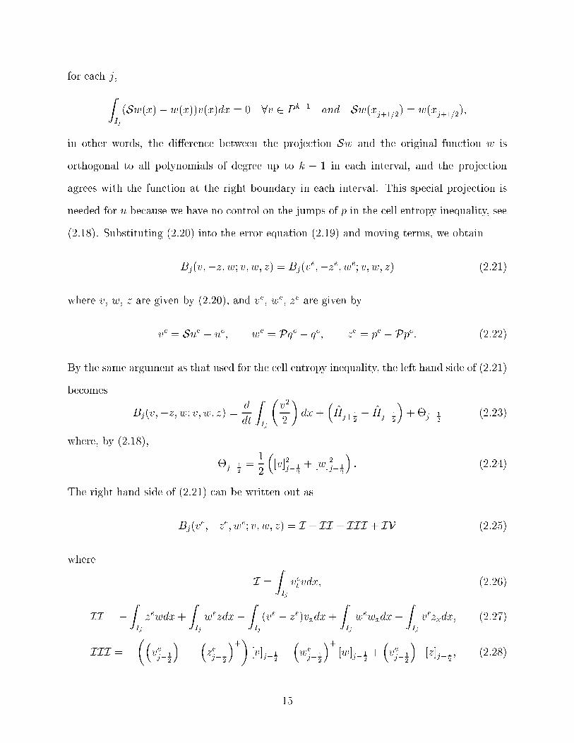
(Sw(x)� w(x))v(x)dx = 0 8v 2 P k�1 and Sw(x�j+1=2) = w(x�j+1=2);

in other words, the di�erence between the projection Sw and the original function w is

orthogonal to all polynomials of degree up to k � 1 in each interval, and the projection

agrees with the function at the right boundary in each interval. This special projection is

needed for u because we have no control on the jumps of p in the cell entropy inequality, see

(2.18). Substituting (2.20) into the error equation (2.19) and moving terms, we obtain

Bj(v;�z; w; v; w; z) = Bj(ve;�ze; we; v; w; z) (2.21)

where v, w, z are given by (2.20), and ve, we, ze are given by

ve = Sue � ue; we = Pqe � qe; ze = pe � Ppe: (2.22)

By the same argument as that used for the cell entropy inequality, the left hand side of (2.21)

becomes

Bj(v;�z; w; v; w; z) = d

dt

ZIj

�v2

2

�dx +

�Hj+ 1

2

� Hj� 1

2

�+�j� 1

2

(2.23)

where, by (2.18),

�j� 1

2

=1

2

�[v]2

j� 1

2

+ [w]2j� 1

2

�: (2.24)

The right hand side of (2.21) can be written out as

Bj(ve;�ze; we; v; w; z) = I + II + III + IV (2.25)

where

I =

ZIj

vet vdx; (2.26)

II = �ZIj

zewdx+

ZIj

wezdx�ZIj

(ve � ze)vxdx+

ZIj

wewxdx+

ZIj

vezxdx; (2.27)

III = ���

vej� 1

2

����zej� 1

2

�+�[v]j� 1

2

+�wej� 1

2

�+[w]j� 1

2

+�vej� 1

2

��[z]j� 1

2

; (2.28)

15

and

IV = hj+ 1

2

� hj� 1

2

(2.29)

for some ux function h. Notice that v; w; z are given by (2.20) and ve; we; xe are given by

(2.22), respectively.

Now, by using the simple inequality ab � 1

2(a2+ b2), and standard approximation theory

on vet = (Sue � ue)t, see, e.g. [6], we have

I � C�x2k+3j +

ZIj

�v2

2

�dx:

Because P is a local L2 projection, and S, even though not a local L2 projection, does

have the property that w � Sw is locally orthogonal to all polynomials of degree up to

k � 1, all the terms in II are actually zero. The last term in III is zero, because of the

special interpolating property of the projection S. An application of the simple inequality

ab � 1

2(a2 + b2) for the �rst two terms in III and standard approximation theory on the

point values of ve � ze = (Sue � ue) + (Ppe � pe) and of we = Pqe � qe (see, e.g. [6]) then

gives

III � C(�x2k+2j�1 +�x2k+2j +1

4

�[v]2 + [w]2

�:

Finally, IV only contains ux di�erence terms which will vanish upon a summation in j.

Combining all these and summing over j we obtain the following inequality

d

dt

Z1

0

�v2

2

�dx +

1

4

�[v]2 + [w]2

� � C�x2k+1 +

Z1

0

�v2

2

�dx:

An integration in t plus the standard approximation theory on ve = Sue� ue then gives the

desired error estimate (2.17).

3 The LDG method for the multiple dimensional case

In this section, we generalize the scheme discussed in the previous section to multiple spatial

dimensions x = (x1; � � � ; xd). We solve the following nonlinear problem:

ut +dX

i=1

fi(u)xi +dX

i=1

r0i(u)

dXj=1

gij(ri(u)xi)xj

!xi

= 0; 0 � xi � 1; i = 1; � � � ; d (3.1)

16

with an initial condition

u(x; 0) = u0(x); 0 � xi � 1; i = 1; � � � ; d (3.2)

and periodic boundary conditions. Here fi(u), ri(u) and gij(q) are arbitrary (smooth) non-

linear functions. Notice that the assumption of a box geometry and periodic boundary

conditions is for simplicity only and is not essential: the method can be easily designed for

arbitrary domain and for non-periodic boundary conditions.

Let's denote a triangulation of the unit box by T�x, consisting of non-overlapping poly-

hedra covering completely the unit box. Hanging nodes are allowed. Here �x measures the

longest edge of all polyhedra in T�x. We again denote the �nite element space by

V d�x = fv : v is a polynomial of degree at most k for x 2 K; 8K 2 T�xg : (3.3)

Similar to the one dimensional case, to de�ne the LDG method, we �rst introduce the

new variables

qi = ri(u)xi; pi =dX

j=1

gij(qi)xj ; i = 1; � � � ; d (3.4)

and rewrite the equation (3.1) as a �rst order system:

ut +dX

i=1

(fi(u) + r0i(u)pi)xi = 0;

pi �dX

j=1

gij(qi)xj = 0; qi � ri(u)xi = 0; i = 1; � � � ; d: (3.5)

The LDG method is obtained by discretizing the above system with the discontinuous

Galerkin method. This is achieved by multiplying the equations in (3.5) by test functions

v; wi; zi respectively, integrate over an element K 2 T�x, and integrate by parts. We again

need to pay special attention to the boundary terms resulting from the procedure of integra-

tion by parts, as in the one dimensional case. Thus we seek piecewise polynomial solutions

u; pi; qi 2 V d�x, where V

d�x is de�ned in (3.3), such that for all test functions v; wi; zi 2 V d

�x

17

we haveZK

utvdx�dX

i=1

ZK

(fi(u) + r0i(u)pi)vxidx +

Z@K

dhnKvintKds = 0;

ZK

piwidx+dX

j=1

ZK

gij(qi)(wi)xjdx�Z@K

[gi;nKwintKds = 0; i = 1; � � � ; d (3.6)Z

K

qizidx+

ZK

ri(u)(zi)xidx�Z@K

dri;nKzintKds = 0; i = 1; � � � ; d;

where @K is the boundary of element K, and the numerical uxes (the \hats") are de�ned

similar to the one dimensional cases, namely

dhnK =\fnK ;K(uintK ; uextK) +

Pdi=1 (ri(u

extK )� ri(uintK)) p+i ni;K

uextK � uintK

[gi;nK =\gi;nK ;K(qintK ; qextK); dri;nK = ri(u

�)ni;K: (3.7)

Here nK = (n1;K; � � � ; nd;K) is the outward unit normal for element K along the element

boundary @K, uintK denotes the value of u evaluated from inside the element K, and uextK

denotes the value of u evaluated from outside the elementK (inside the neighboring element).

On the other hand, p+ denotes the value of p evaluated from a pre-designated \plus" side

along an edge e, which is always the boundaries of two neighboring elements. For example,

we could choose a �xed vector � which is not parallel with any normals of element boundaries,

and then designate the \plus" side to be the side at the end of the arrow of the normal n with

n �� > 0, see Figure 3.1.\fnK ;K(uintK ; uextK) is a monotone ux for fnK(u) =

Pdi=1 fi(u)ni;K,

namely\fnK ;K(uintK ; uextK) is a Lipschitz continuous function in both arguments uintK and

uextK , is consistent with fnK (u) in the sense thatdfnK (u; u) = fnK (u), and is a non-decreasing

function in uintK and a non-increasing function in uextK . Moreover, it is conservative (that

is, there is only one ux at each edge shared by two elements, added to the residue for one

and subtracted from the reside for another), namely

\fnK ;K(a; b) = �\fnK0 ;K0(b; a)

where K and K 0 share the same edge where the ux is computed and hence nK0 = �nK .

Likewise, �\gi;nK ;K(qintKi ; qextKi ) is a monotone ux for �gi;nK (qi) = �Pd

j=1 gij(q)nj;K. Notice

18

β

ββn

n

n

+β

_

+_ +_

Figure 3.1: Illustration of the de�nition of \plus" and \minus" sides determined by a pre-determined vector �.

that we can again use the one dimensional monotone uxes as in the previous section. For

example, we can use the simple Lax-Friedrichs ux

\fnK ;K(uintK ; uextK) =

1

2

dX

i=1

�fi(u

intK) + fi(uextK)

�ni;K � �(uextK � uintK )

!; (3.8)

� = maxujf 0nK(u)j;

where the maximum is taken over a relevant range of u. The algorithm is now well de�ned.

Again, the algorithm (3.6)-(3.7) is very easy for numerical implementation. Given u, one

�rst locally solves for the qi, then locally solves for the pi, and �nally locally solves for the

update of u. All the advantages listed for the method for the one dimensional case are still

valid in this multiple dimensional case.

We still have the following \cell entropy inequality" for the scheme (3.6)-(3.7). The proof

follows the same lines as that for the one dimensional case, so we will omit it.

Proposition 3.1. (cell entropy inequality) There exist conservative numerical entropy uxes

\HnK ;K such that the solution to the scheme (3.6)-(3.7) satis�es

d

dt

ZK

�u2(x; t)

2

�dx+

Z@K

\HnK ;Kds � 0: (3.9)

19

The L2 stability of the method is then again a trivial corollary, by summing up the cell

entropy inequalities over K:

Corollary 3.1. (L2 stability) The solution to the scheme (3.6)-(3.7) satis�es the L2 stability

d

dt

Z

�u2(x; t)

2

�dx � 0: (3.10)

The same cell entropy inequality also holds for the implicit time discretizations:

Proposition 3.2. (implicit time discretization) The cell entropy inequality and the L2

stability also hold for the time discretization (2.13) with 1

2� � � 1 for the scheme (3.6)-

(3.7). That is, ZK

�(un+1(x))2 � (un(x))2

2�t

�dx+

Z@K

\Hn+�nK ;Kds � 0; (3.11)

and Z

(un+1(x))2dx �Z

(un(x))2dx: (3.12)

Unfortunately, we could not get the optimal error estimate because of the lack of a

suitable projection S similar to the one dimensional case. However, numerical examples in

the next section verify that the accuracy holds as in the one dimensional case.

4 Numerical examples

In this section we provide a few preliminary numerical examples to illustrate the accuracy and

capability of the method. Attention has not been paid to eÆciency in time discretizations,

so explicit third order Runge-Kutta method [22] is used. Study of suitable implicit time

discretizations which have eÆcient iterative solvers maintaining the local structure of the

method is the subject of a future study.

20

Table 4.1: ut+ uxxx = 0. u(x; 0) = sin(x). Periodic boundary conditions. L2 and L1 errors.Non-uniform meshes with N cells. LDG methods with k = 0; 1; 2; 3. t = 1.

k N=10 N=20 N=40 N=80error error order error order error order

0 L2 2.2222E-01 1.2014E-01 0.88 6.2532E-02 0.94 3.1900E-02 0.97L1 4.3282E-01 2.2006E-01 0.97 1.1210E-01 0.97 5.8810E-02 0.93

1 L2 2.0144E-02 5.2347E-03 1.94 1.3322E-03 1.97 3.3592E-04 1.98L1 8.8110E-02 2.3302E-02 1.93 5.9387E-03 1.97 1.4969E-03 1.98

2 L2 9.8394E-04 1.1974E-04 3.03 1.4953E-05 3.00 1.8687E-06 3.00L1 5.2984E-03 6.8421E-04 2.95 8.5138E-05 3.00 1.0728E-05 2.99

3 L2 7.3589E-05 4.6509E-06 3.98 2.9191E-06 3.99 2.0141E-08 3.86L1 3.4438E-04 2.2260E-05 3.95 1.3992E-06 3.99 9.1039E-08 3.94

We would like to illustrate through these numerical examples the high order accuracy

of the methods for both one dimensional and two dimensional, both linear and nonlinear

problems. We would also like to illustrate the good behavior of the method for the so-called

convection dominated cases, namely the case where the coeÆcients of the third derivative

terms are small.

Example 4.1. We compute the solution of the linear one dimensional equation

ut + uxxx = 0 (4.1)

with an initial condition u(x; 0) = sin(x) and periodic boundary conditions (with 2� pe-

riodicity). The exact solution is given by u(x; t) = sin(x + t). Both uniform meshes and

non-uniform meshes are used. The non-uniform meshes in this and later examples are a

repeated pattern of 0:9�x and 1:1�x with an even number of elements. The L2 and L1

errors and the numerical order of accuracy are contained in Table 1.1 (in section 1) for the

uniform mesh case, and in Table 4.1 for the non-uniform mesh case. We can clearly see that

the method with P k elements are giving a uniform (k+1)-th order of accuracy in both norms

for both the uniform and the non-uniform meshes.

21

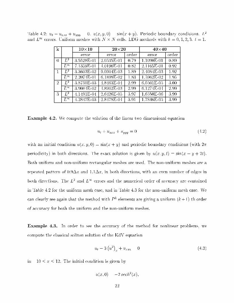
Table 4.2: ut + uxxx + uyyy = 0. u(x; y; 0) = sin(x + y). Periodic boundary conditions. L2

and L1 errors. Uniform meshes with N �N cells. LDG methods with k = 0; 1; 2; 3. t = 1.

k 10�10 20�20 40�40error error order error order

0 L2 3.5528E-01 2.0535E-01 0.79 1.1090E-01 0.89L1 7.1359E-01 4.0190E-01 0.82 2.1165E-01 0.92

1 L2 3.3603E-02 9.0904E-03 1.89 2.4084E-03 1.92L1 2.2074E-01 6.1899E-02 1.83 1.5962E-02 1.95

2 L2 3.8750E-03 4.8463E-04 2.99 6.0501E-05 3.00L1 3.9084E-02 4.8902E-03 2.99 6.1274E-04 2.99

3 L2 4.1491E-04 2.6426E-05 3.97 1.6550E-06 3.99L1 4.2847E-03 2.8478E-04 3.91 1.7846E-05 3.99

Example 4.2. We compute the solution of the linear two dimensional equation

ut + uxxx + uyyy = 0 (4.2)

with an initial condition u(x; y; 0) = sin(x + y) and periodic boundary conditions (with 2�

periodicity) in both directions. The exact solution is given by u(x; y; t) = sin(x + y + 2t).

Both uniform and non-uniform rectangular meshes are used. The non-uniform meshes are a

repeated pattern of 0:9�x and 1:1�x, in both directions, with an even number of edges in

both directions. The L2 and L1 errors and the numerical order of accuracy are contained

in Table 4.2 for the uniform mesh case, and in Table 4.3 for the non-uniform mesh case. We

can clearly see again that the method with P k elements are giving a uniform (k+1)-th order

of accuracy for both the uniform and the non-uniform meshes.

Example 4.3. In order to see the accuracy of the method for nonlinear problems, we

compute the classical soliton solution of the KdV equation

ut � 3�u2�x+ uxxx = 0 (4.3)

in �10 � x � 12. The initial condition is given by

u(x; 0) = �2 sech2(x);

22

Table 4.3: ut + uxxx + uyyy = 0. u(x; y; 0) = sin(x + y). Periodic boundary conditions. L2

and L1 errors. Non-uniform meshes with N � N cells. LDG methods with k = 0; 1; 2; 3.t = 1.

k 10�10 20�20 40�40error error order error order

0 L2 3.5963E-01 2.0788E-01 0.79 1.1228E-01 0.88L1 7.3869E-01 4.0713E-01 0.85 2.1681E-01 0.91

1 L2 3.4590E-02 9.1681E-03 1.92 2.3412E-03 1.97L1 2.5815E-01 7.2978E-02 1.82 1.8533E-02 1.97

2 L2 4.0949E-03 5.1285E-04 2.99 6.4054E-05 3.00L1 5.0429E-02 6.3078E-03 2.99 8.0584E-04 2.97

3 L2 4.5434E-04 2.8854E-05 3.97 1.8080E-06 3.99L1 6.0982E-03 4.0321E-04 3.92 2.5340E-05 3.99

The exact solution is

u(x; t) = �2 sech2(x� 4t):

We compute the solution with two di�erent boundary conditions. Table 4.4 (uniform mesh)

and Table 4.5 (non-uniform mesh) give the errors of numerical solution at t = 0:5 using the

boundary condition

u(�10; t) = g1(t); ux(12; t) = g2(t); uxx(12; t) = g3(t) (4.4)

where gi(t) corresponds to the data from the exact solution. Notice that the LDG method

allows an easy implementation of such boundary conditions. Table 4.6 (uniform mesh)

and Table 4.7 (non-uniform mesh) give the errors of numerical solution using the periodic

boundary conditions. Although the exact solution is not periodic, the large size of the

computational domain allows the usage of periodic boundary conditions with negligible error.

We can see from these tables that the orders of accuracy are comparable to that for the linear

case.

Example 4.4. In order to see the accuracy of the method for nonlinear problems with small

coeÆcient for the third derivative term, we compute the soliton solution of the generalized

23

Table 4.4: The KdV equation ut � 3 (u2)x + uxxx = 0. u(x; 0) = �2 sech2(x). Boundarycondition (4.4). L2 and L1 errors. Uniform meshes with N cells. LDG methods withk = 0; 1; 2; 3. t = 0:5.

k N=40 N=80 N=160 N=320error error order error order error order

0 L2 2.5292E-01 1.9098E-01 0.40 1.3019E-01 0.55 7.9780E-02 0.71L1 9.0170E-01 6.8651E-01 0.39 4.6405E-01 0.56 2.8531E-01 0.70

1 L2 2.6512E-02 4.6652E-03 2.50 1.0108E-03 2.20 2.5906E-04 1.96L1 1.4748E-01 3.4625E-02 2.09 1.1840E-02 1.55 3.3239E-03 1.83

2 L2 1.5317E-03 1.8083E-04 3.08 2.2642E-05 2.99 2.8335E-06 2.99L1 1.7486E-02 2.7505E-03 2.66 3.5575E-04 2.95 4.4397E-05 3.00

3 L2 2.0631E-04 1.3981E-05 3.88 8.9054E-07 3.97 5.6029E-08 3.99L1 2.0155E-03 2.1462E-04 3.23 1.4461E-05 3.89 9.1140E-07 3.98

Table 4.5: The KdV equation ut � 3 (u2)x + uxxx = 0. u(x; 0) = �2 sech2(x). Boundarycondition (4.4). L2 and L1 errors. Non-uniform meshes with N cells. LDG methods withk = 0; 1; 2; 3. t = 0:5.

k N=40 N=80 N=160 N=320error error order error order error order

0 L2 2.4530E-01 1.9004E-01 0.37 1.3390E-01 0.50 8.4635E-02 0.66L1 1.0172E+00 7.6826E-01 0.40 5.3383E-01 0.52 3.3655E-01 0.66

1 L2 2.7042E-02 4.9065E-03 2.46 1.0555E-03 2.21 2.6978E-04 1.97L1 1.4490E-01 4.1570E-02 1.80 1.3925E-02 1.57 3.9129E-03 1.83

2 L2 1.9493E-03 2.0134E-04 3.27 2.4926E-05 3.01 3.1208E-06 2.99L1 2.2876E-02 3.5163E-03 2.70 4.7161E-04 2.89 5.9033E-05 2.99

3 L2 3.0402E-04 1.5462E-05 4.29 1.0064E-06 3.94 6.3370E-08 3.99L1 2.7735E-03 2.1464E-04 3.69 1.8358E-05 3.55 1.3119E-06 3.80

24

Table 4.6: The KdV equation ut � 3 (u2)x + uxxx = 0. u(x; 0) = �2 sech2(x). Periodicboundary condition. L2 and L1 errors. Uniform meshes with N cells. LDG methods withk = 0; 1; 2; 3. t = 0:5.

k N=40 N=80 N=160 N=320error error order error order error order

0 L2 2.5292E-01 1.9098E-01 0.40 1.3020E-01 0.55 7.9822E-02 0.70L1 9.0170E-01 6.8648E-01 0.39 4.6404E-01 0.56 2.8602E-01 0.69

1 L2 2.6600E-02 4.6801E-03 2.50 1.0133E-03 2.20 2.5966E-04 1.96L1 1.4778E-01 3.4403E-02 2.10 1.1930E-02 1.52 3.3404E-03 1.84

2 L2 1.5883E-03 1.8254E-04 3.12 2.2699E-05 3.00 2.8353E-06 3.00L1 1.7729E-02 2.7130E-03 2.70 3.5359E-04 2.94 4.4350E-05 2.99

3 L2 2.1442E-04 1.5566E-05 3.78 1.0318E-06 3.91 6.5818E-08 3.97L1 1.9911E-03 2.2607E-04 3.14 1.5397E-05 3.88 9.7191E-07 3.98

Table 4.7: The KdV equation ut � 3 (u2)x + uxxx = 0. u(x; 0) = �2 sech2(x). Periodicboundary condition. L2 and L1 errors. Non-uniform meshes with N cells. LDG methodswith k = 0; 1; 2; 3. t = 0:5.

k N=40 N=80 N=160 N=320error error order error order error order

0 L2 2.4530E-01 1.9004E-01 0.37 1.3391E-01 0.50 8.4650E-02 0.66L1 1.0172E+00 7.6826E-01 0.40 5.3383E-01 0.52 3.3672E-01 0.66

1 L2 2.7071E-02 4.9216E-03 2.46 1.0581E-03 2.21 2.7039E-04 1.97L1 1.4507E-01 4.1341E-02 1.81 1.3916E-02 1.57 3.9383E-03 1.82

2 L2 2.0350E-03 2.0344E-04 3.32 2.4988E-05 3.02 3.1228E-06 3.00L1 2.2916E-02 3.4702E-03 2.72 4.6922E-04 2.88 5.8972E-05 2.99

3 L2 3.2212E-04 1.8451E-05 4.12 1.1715E-06 3.97 7.4102E-08 3.98L1 2.8274E-03 2.2498E-04 3.65 1.9437E-05 3.53 1.3793E-06 3.81

25

Table 4.8: The GKdV equation (4.5) with initial condition (4.6) and boundary condition(4.7). L2 and L1 errors. Non-uniform meshes with N cells. LDG methods with k = 0; 1; 2; 3.t = 1.

k N=160 N=320 N=640 N=1280error error order error order error order

0 L2 1.6566E-02 1.1259E-02 0.56 7.0817E-03 0.67 4.1526E-03 0.77L1 9.3056E-02 6.6829E-02 0.48 4.4502E-02 0.58 2.7539E-02 0.69

1 L2 3.8554E-04 6.0675E-05 2.66 1.1784E-05 2.36 2.8635E-06 2.04L1 3.2635E-03 6.2508E-04 2.38 2.2689E-04 1.47 6.4595E-05 1.81

2 L2 8.2907E-06 9.5348E-07 3.12 1.1895E-07 3.00 1.5290E-08 2.96L1 1.6684E-04 2.2545E-05 2.88 3.0858E-06 2.87 3.9503E-07 2.97

3 L2 1.7005E-06 1.3664E-07 3.63 3.0527E-09 5.48 1.9206E-10 3.99L1 1.7607E-05 1.3291E-06 3.72 8.3962E-08 3.98 5.2861E-09 3.99

KdV equation [5]

ut + ux +

�u4

4

�x

+ �uxxx = 0; (4.5)

in �2 � x � 3, where we take � = 0:2058� 10�4. The initial condition is given by

u(x; 0) = Asech2

3 (K(x� x0)) (4.6)

with A = 0:2275, x0 = 0:5, and K = 3�

A3

40�

� 1

2

. The exact solution is

u(x; t) = Asech2

3 (K(x� x0)� !t)

where ! = K�1 + A3

10

�. We compute the solution using the boundary condition

u(�2; t) = g1(t); ux(3; t) = g2(t); uxx(3; t) = g3(t) (4.7)

with a non-uniform mesh. The result is contained in Table 4.8.

Example 4.5. In this example we compute the classical soliton solutions of the KdV

equation

ut +

�u2

2

�x

+ �uxxx = 0: (4.8)

The examples are those used in [14].

26

The single soliton case has the initial condition

u0(x) = 3c sech2 (k(x� x0)) (4.9)

with c = 0:3, x0 = 0:5, k = (1=2)pc=� and � = 5 � 10�4. The solution is computed in

x 2 [0; 2] with periodic boundary conditions, using P 2 elements with 100 cells, and is shown

in Figure 4.1.

The double soliton collision case has the initial condition

u0(x) = 3c1 sech2 (k1(x� x1)) + 3c2 sech

2 (k2(x� x2)) (4.10)

with c1 = 0:3, c2 = 0:1, x1 = 0:4, x2 = 0:8, ki = (1=2)pci=� for i = 1; 2, and � = 4:84�10�4.

The solution is computed in x 2 [0; 2] with periodic boundary conditions, using P 2 elements

with 100 cells. and is shown in Figure 4.2.

The triple soliton splitting case has the initial condition

u0(x) =2

3sech2

�x� 1p108�

�(4.11)

with � = 10�4. The solution is computed in x 2 [0; 3] with periodic boundary conditions and

is shown in Figure 4.3.

Example 4.6. We compute in this example the KdV zero dispersion limit of conservation

laws. The equation is (4.8) with an initial condition

u(x; 0) = 2 + 0:5 sin(2�x) (4.12)

for x 2 [0; 1] with periodic boundary conditions, and we are interested in the limit when

� ! 0+. Theoretical and numerical discussions about this limit can be found in [19] and

[23]. Here we are mainly concerned with the capability of our numerical method in resolving

the small scale solution structures in this limit when � is small. For this purpose we compute

the solution to t = 0:5 with � = 10�4; 10�5; 10�6 and 10�7 using P 2 elements with 300 cells

for the �rst two cases, 800 cells for the third case and 1700 cells for the last case. We have

veri�ed that these are \converged" solutions in the sense that further increasing the number

27

x

u

0 0.5 1 1.5 2

0

0.1

0.2

0.3

0.4

0.5

0.6

0.7

0.8

0.9

1t = 0

x

u0 0.5 1 1.5 2

0

0.1

0.2

0.3

0.4

0.5

0.6

0.7

0.8

0.9

1t = 1

x

u

0 0.5 1 1.5 2

0

0.1

0.2

0.3

0.4

0.5

0.6

0.7

0.8

0.9

1t = 2

0 0.5 1 1.5 2x0

1

2

3

t

Figure 4.1: Single soliton pro�les. Solutions of equation (4.8) with initial condition (4.9) andperiodic boundary conditions in [0,2] using P 2 elements with 100 cells. Top left: solution att = 0; top right: t = 1; bottom left: t = 2; bottom right: space time graph of the solutionup to t = 3.

28

x

u

0 0.5 1 1.5 2

0

0.1

0.2

0.3

0.4

0.5

0.6

0.7

0.8

0.9

1

t = 0

x

u0 0.5 1 1.5 2

0

0.1

0.2

0.3

0.4

0.5

0.6

0.7

0.8

0.9

1t = 1

x

u

0 0.5 1 1.5 2

0

0.1

0.2

0.3

0.4

0.5

0.6

0.7

0.8

0.9

1t = 2

00.5

11.5

2 0

1

2

3

4

t

Figure 4.2: Double soliton collision pro�les. Solutions of equation (4.8) with initial condition(4.10) and periodic boundary conditions in [0,2] using P 2 elements with 100 cells. Top left:solution at t = 0; top right: t = 1; bottom left: t = 2; bottom right: space time graph of thesolution up to t = 4.

29

x

u

0 1 2 3

0

0.1

0.2

0.3

0.4

0.5

0.6

0.7

0.8

0.9

1

t = 0

x

u0 1 2 3

0

0.1

0.2

0.3

0.4

0.5

0.6

0.7

0.8

0.9

1

t = 1

x

u

0 1 2 3

0

0.1

0.2

0.3

0.4

0.5

0.6

0.7

0.8

0.9

1

t = 2

0 1 2 3x0

1

2

3

4

t

Figure 4.3: Triple soliton splitting pro�les. Solutions of equation (4.8) with initial condition(4.11) and periodic boundary conditions in [0,3] using P 2 elements with 150 cells. Top left:solution at t = 0; top right: t = 1; bottom left: t = 2; bottom right: space time graph of thesolution up to t = 4.

30

of cells does not change the solutions graphically. These solutions are shown in Figure 4.4.

Notice the physical \oscillations" which are typical in such dispersive limits, see, e.g. [19].

Clearly our method is very suitable to compute such solutions.

5 Concluding remarks

We have designed a class of local discontinuous Galerkin methods for solving KdV type equa-

tions containing third derivatives and have proven their stability for any spatial dimensions

for a general class of nonlinear equations. Numerical examples are shown to illustrate the

accuracy and capability of the methods, especially for the convection dominated cases where

the coeÆcients of the third derivative terms are small. EÆcient implicit time discretizations

which have eÆcient iterative solvers maintaining the local structure of the method, accuracy

enhancement study, and more numerical experiments with physically interesting problems

constitute an ongoing project.

Acknowledgments. We would like to thank Bernardo Cockburn for his valuable help in

the discussion about the projection S, and Andy Majda for pointing out reference [19] and

test cases of zero dispersive limits of conservation laws in Example 4.6.

References

[1] T. B. Benjamin, J. L. Bona and J. J. Mahony, Model equations for long waves in

nonlinear, dispersive systems, Phil. Trans. Roy. Soc. Lond. A, v272 (1972), pp.47-78.

[2] F. Bassi and S. Rebay, A high-order accurate discontinuous �nite element method for

the numerical solution of the compressible Navier-Stokes equations, J. Comput. Phys.,

v131 (1997), pp.267-279.

[3] R. Biswas, K. D. Devine and J. Flaherty, Parallel, adaptive �nite element methods for

conservation laws, Appl. Numer. Math., v14 (1994), pp.255-283.

31

x

u

0 0.25 0.5 0.75 11.4

1.6

1.8

2

2.2

2.4

2.6

2.8

3

3.2

3.4P2, ε=10-4, t=0.5, n=300

x

u

0 0.25 0.5 0.75 11.4

1.6

1.8

2

2.2

2.4

2.6

2.8

3

3.2

3.4P2, ε=10-5, t=0.5, n=300

x

u

0 0.25 0.5 0.75 11.4

1.6

1.8

2

2.2

2.4

2.6

2.8

3

3.2

3.4P2, ε=10-6, t=0.5, n=800

x

u

0 0.25 0.5 0.75 11.4

1.6

1.8

2

2.2

2.4

2.6

2.8

3

3.2

3.4P2, ε =10-7, t=0.5, n=1700

Figure 4.4: Zero dispersion limit of conservation laws. Solutions of equation (4.8) with initialcondition (4.12) and periodic boundary conditions in [0,1] using P 2 elements at t = 0:5. Topleft: � = 10�4 with 300 cells; top right: � = 10�5 with 300 cells; bottom left: � = 10�6 with800 cells; bottom right: � = 10�7 with 1700 cells.

32

[4] J. L. Bona, V. A. Dougalis and O. A. Karakashian, Fully discrete Galerkin methods for

the Korteweg-de Vries equation, Comput. Math. Appl., v12A (1986), pp.859-884.

[5] J. L. Bona, V. A. Dougalis, O. A. Karakashian and W. R. McKinney, Conservative, high-

order numerical schemes for the generalized Korteweg-de Vries equation, Phil. Trans.

Roy. Soc. Lond. A, v351 (1995), pp.107-164.

[6] P. Ciarlet, The �nite element method for elliptic problems, North Holland, 1975.

[7] B. Cockburn, S. Hou, and C.-W. Shu, TVB Runge-Kutta local projection discontinuous

Galerkin �nite element method for conservation laws IV: the multidimensional case,

Math. Comp., v54 (1990), pp.545-581.

[8] B. Cockburn, G. Karniadakis and C.-W. Shu, The development of discontinuous

Galerkin methods, in Discontinuous Galerkin Methods: Theory, Computation and Appli-

cations, B. Cockburn, G. Karniadakis and C.-W. Shu, editors, Lecture Notes in Compu-

tational Science and Engineering, volume 11, Springer, 2000, Part I: Overview, pp.3-50.

[9] B. Cockburn, S.-Y. Lin and C.-W. Shu, TVB Runge-Kutta local projection discontinuous

Galerkin �nite element method for conservation laws III: one dimensional systems, J.

Comput. Phys., v84 (1989), pp.90-113.

[10] B. Cockburn and C.-W. Shu, TVB Runge-Kutta local projection discontinuous Galerkin

�nite element method for scalar conservation laws II: general framework, Math. Comp.,

v52 (1989), pp.411-435.

[11] B. Cockburn and C.-W. Shu, TVB Runge-Kutta local projection discontinuous Galerkin

�nite element method for scalar conservation laws V: multidimensional systems, J. Com-

put. Phys., v141 (1998), pp.199-224.

33

[12] B. Cockburn and C.-W. Shu, The local discontinuous Galerkin method for time-

dependent convection di�usion systems, SIAM J. Numer. Anal., v35 (1998), pp.2440-

2463.

[13] B. Cockburn and C.-W. Shu, Runge-Kutta Discontinuous Galerkin methods for

convection-dominated problems, submitted to J. Sci. Comput.

[14] A. Debussche and J. Printems, Numerical simulation of the stochastic Korteweg-de Vries

equation, Physica D, v134 (1999), pp.200-226.

[15] C.L. Gardner, The quantum hydrodynamic model for semiconductor devices, SIAM J.

Appl. Math., v54 (1994), pp.409-427.

[16] G.-S. Jiang and C.-W. Shu, On cell entropy inequality for discontinuous Galerkin meth-

ods, Math. Comp., v62 (1994), pp.531-538.

[17] O. A. Karakashian and W. R. McKinney, On the approximation of solutions of the

generalized Korteweg-de Vries equation, Math. Comput. Simulation, v37 (1994), pp.405-

416.

[18] D. J. Korteweg and G. de Vries, On the change of form of long waves advancing in a

rectangular canal and on a new type of long stationary waves, Philosophical Magazine,

v39 (1895), pp.422-443.

[19] P. D. Lax, C. D. Levermore and S. Venakides, The generation and propagation of os-

cillations in dispersive initial value problems and their limiting behavior, in Important

Developments in Soliton Theory, Springer Series in Nonlinear Dynamics, A.S. Fokas and

V.E. Zakharov, Eds., Springer-Verlag, 1993, pp.205-241.

[20] W. H. Reed and T. R. Hill, Triangular mesh methods for the neutron transport equation,

Tech. Report LA-UR-73-479, Los Alamos Scienti�c Laboratory, 1973.

34

[21] C.-W. Shu, TVB uniformly high-order schemes for conservation laws, Math. Comp.,

v49 (1987), pp.105-121.

[22] C.-W. Shu and S. Osher, EÆcient implementation of essentially non-oscillatory shock

capturing schemes, Journal of Computational Physics, v77 (1988), pp.439-471.

[23] S. Venakides, The zero dispersion limit of the Korteweg-de Vries equation with periodic

initial data, AMS Trans. v301 (1987), pp.189-225.

35