1 executive summary 2 project overview 3 platinum market ... · d0034.2004-01-06 pgm final...

0D0034.2004-01-06 PGM Final Report.ppt

Table of Contents

Project Overview

3

4

5 Econometric Modeling

2

Platinum Market Overview

66

1 Executive Summary

Future Demand Scenarios 2005-2050

AppendixAppendix


AppendixAppendix

Summary of Previous Studies

Econometric Analyses

Vehicle Forecasts

Stationary Fuel Cell Markets

Platinum Mining


AppendixPrevious Studies Introduction

Several studies have modeled fuel cell vehicle market penetration and its effect on platinum availability.

19 g Pt

22 g Pt

Low - 5 g Pt

Study g Pt per FCV FCV Market Penetration

100% penetration in 2100 (global)

400 million FCV annual production

Best case: 100% in 2070 (US fleet growth = 25.3 million

FCV/year in 2050)

Råde Doctoral ThesisChalmers University of Technology & Göteborg University, 2001

BorgwardtU.S. Environmental Protection Agency

Transportation Research Part DJournal Article, 2001

Tonn and DasOak Ridge National Laboratory

Assessment of platinum availability for advanced fuel cell vehicles.Report, 2001

50 kW

50 kW

50 kW

Overview of Platinum Availability StudiesOverview of Platinum Availability StudiesFCV Power FCV Life

Two scenarios:

1) 50% penetration in 2050

2) 80% penetration in 2050

TIAX LLC, 2003 10 year life, plus recycling at 95% efficiency

60 g Pt (2005)

15 g Pt (2025)75 kW

10 year life, plus recycling

15 year life,plus recycling Worst case: 100% in 2150

(US fleet growth = 10 million FCV/year in 2150)

Low - 6% in 2030 (US)

Recycling at FCV end of life

Med - 20% in 2030 (US)Med - 10 g Pt

14 g Pt Assumes 1 billion FCVs in 2030, Worldwide

World Fuel Cell Council(Formerly the Platinum Association) 70 kW

High - 60% in 2030 (US)High - 30 g Pt

10 year life, plus recycling


AppendixPrevious Studies Resource Estimates

Most published studies indicate that platinum availability will be a concern.

Study Conclusions

“In the baseline scenario, the demand for primary platinum in the 21st century amounts to 156 Gg, and current reserves and identified resources of platinum would be depleted in the 2050’s and 2060’s, respectively.”

Unrestricted US fleet conversion to FCVs would require 66 years and 10,800 tonnes of Pt. If US Pt consumption remains at its current level of 16% of annual world production, fleet conversion would require 146 years and 15,200 tonnes of Pt.

“These results imply that, without alternative catalysts, fuel cells alone cannot adequately address the issue facing the current system of road transport.”

Under the worst case scenario, half of known PGM reserves are exhausted before mid-century. This scenario is characterized by a high demand for new vehicles in the developing countries and high penetration of reformer-equipped fuel cell vehicles with relatively high amounts of PGMs.

“At an increase consumption rate of 6% per year, there are adequate indicated resources of PGE in the Bushveld Complex alone to supply demand for the next 50 years.”

Overview of Platinum Availability StudiesOverview of Platinum Availability StudiesResources

67 Gg in Pt resources

Råde Doctoral ThesisChalmers University of Technology

& Göteborg University, 2001

47,500 tonnes(47.5 Gg) in Pt

resources

BorgwardtU.S. Environmental Protection Agency

Transportation Research Part DJournal Article, 2001

Tonn and DasOak Ridge National Laboratory

Assessment of platinum availability for advanced fuel cell vehicles.Report, 2001

100 Gg in PGM reserves

~50 Gg in Pt reserves1

4,705 Mozs in PGM deposits

~73 Gg in Pt deposits1

1TIAX estimate based on 50% Pt in total PGM resources and 31.1 g/oz

World Fuel Cell Council(Formerly the Platinum Association)

1 billion car fleet corresponds 450 million troy ounces of platinum.With 95% recycling, 2 million troy ounces a year required to maintain global fleet (currently, autocatalyst requires 1.6 million/yr).

1.5 billion troz (47 Gg) in Pt

resources

CawthornUniversity of WitwatersrandGlobal Platinum and Palladium DepositsReview, 2001


AppendixAppendix



Vehicle Forecasts


Platinum Mining


AppendixEconometric Analyses Introduction

We conducted a series of econometric analyses to model platinum supply, demand and price.

• Platinum Jewelry Demand: Both Japan and the world1

• Total World Demand for Platinum: All uses of platinum2

Econometric AnalysesEconometric Analyses

• Platinum Supply3

• World demand for autocatalyst and investment were not modeled separately because:– Price elasticity of demand for platinum from autocatalyst is derived from a conceptual

model of the general equilibrium derived demand.- Autocatalyst use is required by regulation.- Autocatalyst accounts for only a very small proportion of total car manufacturing

costs. – Investment demand for platinum only accounts for a relative small proportion of total

demand for platinum.


AppendixEconometric Analyses Platinum Jewelry Demand

Platinum Jewelry Demand: Japan has been the largest market for platinum jewelry, but demand has been affected by Japan’s economic slowdown. In the meantime, platinum jewelry demand has grown sharply in China, reaching 1.3 million troy ounces (40 Mg) in 2001.

0.0%

10.0%

20.0%

30.0%

40.0%

50.0%

60.0%

70.0%

80.0%

90.0%

100.0%

1975 1980 1985 1990 1995 2000

North AmericaJapanEuropeROW

Year

Jew

elry

Dem

and

(%)

Largely due to increased China demand

Jewelry Market Share by Region (%)Jewelry Market Share by Region (%)

Source: Johnson Matthey, Platinum 2001.



The predictive power of the jewelry demand model based on the Japanese market can be questioned given Japan’s decreasing share in the world platinum jewelry market. However, we believe that the model provided valuable insight into market dynamics.

• The jewelry demand model helps to illustrate the relationship between demand and other economic variables and estimate the potential impact of these variables on the demand for platinum jewelry.

• There are similarities in the development of the platinum jewelry market in Japan and China:– Both governments had restrictions on gold ownership that gave an

opportunity for platinum to penetrate into these jewelry markets. The subsequent lifting of restrictions allowed more substitution between platinum and gold jewelry.

– Both countries have experienced rapid economic growth and newly created wealth drives jewelry markets.



The following factors were included in our models of platinum jewelry demand for the world and Japan.• Quantity of demand for platinum jewelry

• GDP (gross domestic product)

• Price of platinum

• Price of gold

• Inflation

• The amount of promotion (advertising) is also an important factor in this market segment; however, this information was not available for analysis.


AppendixEconometric Analyses Platinum Jewelry Demand Model Specification

The jewelry demand models for the world and Japan were specified as follows:

1 1, 2 , 3 4 5 ,, inft j t j t pt t t t Au tnD nD nP nGDP n l nPα β β β β β ε−= + + + + + +l l l l l l

PreviousDemand

PriceEffect

IncomeEffect

Other PriceEffect

InflationEffect

Demand

Quantity of demand for platinum jewelry at time t

Impact of previous platinum jewelry consumption on current quantity of jewelry demand

Dt,j β1Quantity of demand for platinum jewelry at time t-1Dt-1,j

Price elasticity of demand for platinum jewelry—measures the sensitivity of quantity demanded to a price change

β2GDPt Gross Domestic Product at time t

Income elasticity of demand for platinum jewelry—measures the sensitivity of platinum jewelry consumption to an income change

Pt,pt Platinum price at time tβ3

Pt,Au Price of gold at time tMeasures the sensitivity of quantity demanded to a change in inflationβ4Inflt Inflation at time t

Cross price elasticity of demand of platinum jewelry with respect to gold price—measures the sensitivity of platinum demand to a change in gold price

Quantity of demand for platinum jewelry given other variables are equal to zero

β5α


AppendixEconometric Analyses Platinum Jewelry Demand Model Estimation & Statistical Inference

The world and Japan jewelry demand models produced the followingestimated parameters and standard deviations, helping to identify the impact of each factor on the direction and magnitude of platinum jewelry demand.

Demand PreviousDemand

PriceEffect

IncomeEffect

InflationEffect

αα ββ11 ββ22 ββ33 ββ44

tttpttjtjt lnnGDPnPnDnD εββββα +++++= − inf43,2,11, λλλλλ

Worldshort-run*(std.dev.)

5.39(1.42)

0.48(0.13)

-0.33(0.09)

0.92(0.25)

0. 20(0.90)

Worldlong-run*(std. Dev.)

-0.636(0.04)

1.77(0.44)10.37 NA Insignificant

Japan(std.dev.)

-7.19(1.07)

-0.62(0.10)

0.62(0.10)

0.93(1.43)NA

* The chronological definition provided for “short-run” and “long-run” is not precise. The general purpose of the distinction is to differentiate between a short period, where it is impossible for consumers to make adjustments, and a longer period, where consumers have more freedom to make adjustments.

Note: The parameters for the short-run jewelry demand were estimated from the data. Parameters for the “long-run” jewelry demand were derived by adjusting short-run estimates based on the previous year’s jewelry consumption.


AppendixEconometric Analyses Platinum Jewelry Demand World Demand Prediction

The predictive power of the world platinum jewelry demand model was verified by predicting the quantity demanded outside the sample period. • We pretended that the quantity demanded for platinum jewelry was not available from

1999 to 2000 and the model was used to forecast those two years. We then compared the real quantity of demand for platinum jewelry with the model predictions.

• The differences were about 10%.

Qua

ntity

Dem

and

for

Plat

inum

Jew

elry

(troy

oz.

)

0

500000

1000000

1500000

2000000

2500000

3000000

3500000

1975 1980 1985 1990 1995 2000

Actual Jewelry Demand

Prediction

Year

Actual World Jewelry Demand vs. Model’s PredictionActual World Jewelry Demand vs. Model’s Prediction


AppendixEconometric Analyses Platinum Jewelry Demand Japan Demand Prediction

The predictive power of the Japan demand model was verified by predicting quantity demanded for platinum jewelry outside the sample period. • We pretended that the quantity demanded for platinum jewelry was not available from

1999 to 2000 and the model was used to forecast for these two years. Then we compared the real quantity of demand for platinum jewelry with the model predictions.

• The differences were about 0.1%.

Actual Japan Jewelry Demand vs. Model’s PredictionActual Japan Jewelry Demand vs. Model’s Prediction

1.0031.0041.0051.0061.0071.008

1.0091.01

1.0111.0121.013

1975 1980 1985 1990 1995 2000

Actual Jewelry Demand/Per Capita

Prediction

Year

Per C

apita

Dem

and

for

Plat

inum

Jew

elry

(troy

oz.

)


AppendixEconometric Analyses Platinum Jewelry Demand Price Elasticity of Demand

The demand for platinum jewelry is not elastic1, i.e., even when the price is high the quantity demanded will remain high.

• Both the world’s and Japan’s price elasticities of demand for platinum jewelry are inelastic (-0.33 and -0.62 in short-run, and -0.63 for the World in long-run). That is, a 1 percent increase in price will result in a 0.33 to 0.63 percent decline in demand.

• Several publications have stated that demand for platinum jewelry is elastic. – “Demand for platinum in jewelry, its number one use, is ostensibly fairly elastic in that

there are ready substitutes such as gold, white gold, silver and plated precious metal coatings.”2

• Overstated price elasticity may result from misconceptions rather than data analysis. These authors may believe that platinum jewelry is not a necessity and, therefore, the price elasticity of demand for platinum jewelry would be high.

• The less elastic demand of platinum jewelry can be attributed to the fact that demand is driven by the bridal market, which is less price sensitive since the cost of a wedding ring only accounts for a small share of the wedding cost.

1) For the price to be considered “elastic”, a 1 percent increase in price would result in a decline in demand of more than 1 percent.2) Pearse, Gary H.K., Equapolar Publications, “Platinum Group Metals World Resources Economics of the Future”


AppendixEconometric Analyses Platinum Jewelry Demand Influence of Inflation

The model does not indicate that there is a statistically significant relationship between platinum jewelry demand and inflation.• Estimates of the impact of inflation on platinum jewelry demand for both the

world and Japan yielded positive signs, i.e., the quantity demanded could be positively correlated with inflation.

• However, neither estimate is statistically significant.


AppendixEconometric Analyses Platinum Jewelry Demand Cross Price Elasticity

We were not able to estimate the cross price elasticity between gold and platinum jewelry because the price of gold and platinum are highly correlated during the period of this study (the coefficient of correlation is about 0.8).

0

100

200

300

400

500

600

700

800

1975 1980 1985 1990 1995 2000

Platinum

Gold

Year

Pric

e pe

r Tro

y O

z. (U

S D

olla

rs)

Prices of Platinum vs. GoldPrices of Platinum vs. Gold


AppendixEconometric Analyses Platinum Jewelry Demand Cross Price Elasticity

Even though we were not able to estimate the cross price elasticity between gold and platinum jewelry, substitution between platinum and gold* is well known and has been observed by the International Platinum Association.

• “…the recent economic decline in Japan coupled with a widening disparity between the price of gold and platinum together with technical improvements have led recently to increasing substitution of white gold for platinum…”

• “Another element in the success of platinum jewelry in China has been the successful promotion campaign of the Platinum International Guild. However, these campaigns have not yet established the wedding market to anywhere near the same extent as in Japan. Platinum jewelry in China has much more of a fashion element attached to it making it more susceptible to price sensitivity and substitution by white gold than Japan”**

* The price of gold and platinum were highly correlated during the period of the study. The correlation coefficient is about 0.8.

** International Platinum Association, letter from Marcus Nurdin to Eric Carlson (TIAX), 12/13/02.


AppendixEconometric Analyses Total World Demand for Platinum

Total World Demand for Platinum: The objective of our analysis of the world platinum demand was to better understand the relationship between platinum demand and other economic variables across all markets.

• The following factors were addressed in our model of world platinum demand:– GDP (gross domestic product)– Price of platinum– Price of palladium


AppendixEconometric Analyses Total World Demand for Platinum Model Specification

The model of total world demand for platinum model was specified as follows:


PriceEffect

IncomeEffect

Other PriceEffect

tpdttpttpttptt nPnGDPnPnDnD εββββα +++++= − ,43,211 ,, λλλλλ

Dt,pt Total world demand for platinum at time t Impact of previous platinum demand on current quantity of platinum demandβ1

Dt-1,pt Total world demand for platinum at time t-1Price elasticity of demand for platinum—measures the sensitivity of quantity demanded to a platinum price change

β2GDPt Gross Domestic Product at time t

Income elasticity of demand for platinum—measures the sensitivity of platinum demanded to a change in income

Pt,pt Platinum price at time tβ3

Pt,pd Palladium price at time t

Cross price elasticity of demand for platinum with respect to palladium price—measures the sensitivity of quantity demand for platinum to a change in palladium price

Total world demand for platinum given other variables are equal to zero

β4α


Appendix

Econometric Analyses Total World Demand for Platinum Model Estimation & Statistical Inference

The total world platinum demand model produced the following estimated parameters and their standard deviations.


PriceEffect

IncomeEffect

Other PriceEffect

αα ββ11 ββ22 ββ33 ββ44

tpdttpttpttptt nPnGDPnPnDnD εββββα +++++= − ,43,2,11, λλλλλ

Worldshort-run*(std. dev.)

4.66(2.24)

0.70(0.20)

-0.344(0.12)

0.25(0.20)

0. 20(0.12)

Worldlong-run*(std. dev.)

-1.15(0.18)

0.83(0.63)

0.66(0.12)NA NA

* The chronological definition provided for “short-run” and “long-run” is not precise. The general purpose of the distinction is to differentiate between a short period, when it is impossible for consumers to make adjustments, and a longer period, when consumers have more freedom to make adjustments.

Note: The parameters for the short-run jewelry demand model were estimated from the data. Parameters for the “long-run” jewelry demand model were derived from the short-run parameters by adjusting estimates based on the previous year’s jewelry consumption.


AppendixEconometric Analyses Total World Demand for Platinum Prediction

The predictive power of the total world platinum demand model was verified by predicting the quantity demanded outside the sample period. • We pretended that the total quantity of demand was not available from 1999 to 2000 and

the model was used to forecast those two years. We then compared the real total quantity of demand with the model predictions.

• The differences, about 25%, are larger than the differences observed in the predictions of the other two models because of the use of highly aggregated data in this model.

Year

Tota

l Dem

and

for

Plat

inum

(troy

oz.

)

0

1000000

2000000

3000000

4000000

5000000

6000000

7000000

8000000

9000000

10000000

1975 1980 1985 1990 1995 2000

Actual Platinum Demand

Prediction

Actual World Total Platinum Demand vs. Model’s PredictionActual World Total Platinum Demand vs. Model’s Prediction


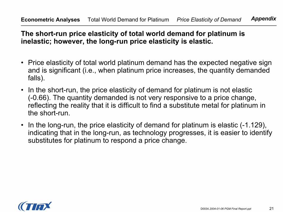
AppendixEconometric Analyses Total World Demand for Platinum Price Elasticity of Demand

The short-run price elasticity of total world demand for platinum is inelastic; however, the long-run price elasticity is elastic.

• Price elasticity of total world platinum demand has the expected negative sign and is significant (i.e., when platinum price increases, the quantity demanded falls).

• In the short-run, the price elasticity of demand for platinum is not elastic (-0.66). The quantity demanded is not very responsive to a price change, reflecting the reality that it is difficult to find a substitute metal for platinum in the short-run.

• In the long-run, the price elasticity of demand for platinum is elastic (-1.129), indicating that in the long-run, as technology progresses, it is easier to identify substitutes for platinum to respond a price change.


AppendixEconometric Analyses Total World Demand for Platinum Income Elasticity of Demand

The total world demand for platinum responds positively to the performance of the world economy—the quantity demanded increases as the total income increases.

• However, the two factors that influence the total world platinum demand (i.e., the world GDP index and the total world platinum demand in previous periods) are highly correlated (coefficient of correlation is about 0.85). As a result, the standard error for income elasticity is very large.

0

2

4

6

8

10

12

14

16

18

1975 1980 1985 1990 1995 2000

Year

Log

(GD

P) &

Log

(Dem

and

for

Plat

inum

at t

-1) Log(GDP)

Log(Demand forPlatinum at t-1)


Appendix

Econometric Analyses Total World Demand for Platinum Cross Price Elasticity of Demand

The cross price elasticity of platinum with respect to palladium is larger in the long-run than in the short-run.

• Unlike the relationship between platinum price and gold price, platinum price and palladium price are not highly correlated during the period we studied. Therefore, we are able to estimate the cross price elasticity of platinum demand with respect to the palladium price.

• The cross price elasticity has the expected positive sign and is significant, indicating that the two metals are substitutes in some applications, such as catalytic converters.

• In the short run, the degree of substitution is small (0.19), i.e., a 1 percent increase in the price of palladium will result in a 0.19 percent increase in demand for platinum. The low level of substitution is due to time, cost and technical limitations.

• In the long run, the degree of substitution increases (0.65), i.e., a 1 percent increase in the price of palladium will result in a 0.65 percent increase in demand for platinum. The level of substitution is higher because of the time available for users to adopt new technology.


AppendixEconometric Analyses Platinum Supply

Platinum Supply: The objective of our analysis of platinum supply was to better understand the relationship between platinum price and supply.

• We were not able to develop a structural model for platinum supply because needed information was not available. A structural model would need to include the information described below:– Proven reserves– Mine and refinery capacity– Mine and refinery capacity utilization– Production cost– Changes in inventory– Secondary supply



Due to the lack of information needed to estimate a complete structural platinum supply model, two related analyses were pursued.

• Analyze the real platinum price on world market. – We conclude that there is no strong evidence that real platinum prices

have trended upward during the 20th century. This result suggests that platinum supply is elastic and future increases in demand for platinum can be met without large change in real price.

• Estimate a distributed lag relationship between real platinum price series and quantities produced.– An exogenous increase in platinum production is modeled as affecting

current platinum price through its effect on the current marginal costs of mining and refining. Such an increase could continue to affect platinum price for some period into the future because of the time required to adjust capital stocks to new levels of price.

1

2



While platinum production has trended up for the period of the study, the real price of platinum has been fairly constant.

1964 1968 1972 1976 1980 1984 1988 1992 1996 20000.0

0.2

0.4

0.6

0.8

1.0

1.2

Rea

l Ran

d pe

r Tro

y O

unce

x 10

4

World production (scaled to fit)South Africa Price (Real rand/troy oz.)

Sources: Production: Johnson Matthey

Price: U.S. Geological Survey South Africa producer price index, South Africa Reserve Bank

Wor

ld P

rodu

ctio

n (M

g)

20

40

60

80

100

120

140

160

World Production and Real SA pt Price: 1960World Production and Real SA pt Price: 1960--20002000


AppendixEconometric Analyses Platinum Supply Model Specification

An inverse platinum supply function is specified to include the time that the industry takes to increase supplies following an increased, permanent change in demand on the right-hand and the level of price on the left-hand side.

• The response to a permanent change in Qt (say due to increased fuel cell use) would be ao in the first year, a1 in the second year, etc. If it took five years for the platinum industry to arrive at the long run desired production level, then the price effects would be non-zero for five years and zero thereafter.

ttttttot DMQQaQQaP ε+++−+−= −−− ...)()( 2111

Real USGS (dollar-denominated) platinum price multiplied by the South African randequivalent of the U.S. dollar and divided by the South African Producer Price Index.Pt

Qt, Qt-1, Qt-2, Qt-1 Contemporaneous quantity of world production and its lags.

Dummy variable indicating years in which there were supply interruptions. The years in which the supply disruption variable equal one is 1965-1968, 1978-1980, 1986, and 1997-1999. In all, the supply disruption dummy variable equals one for 31% of the 35-year sample period.

DMt

ao, a1, an Price response to a permanent change in quantity


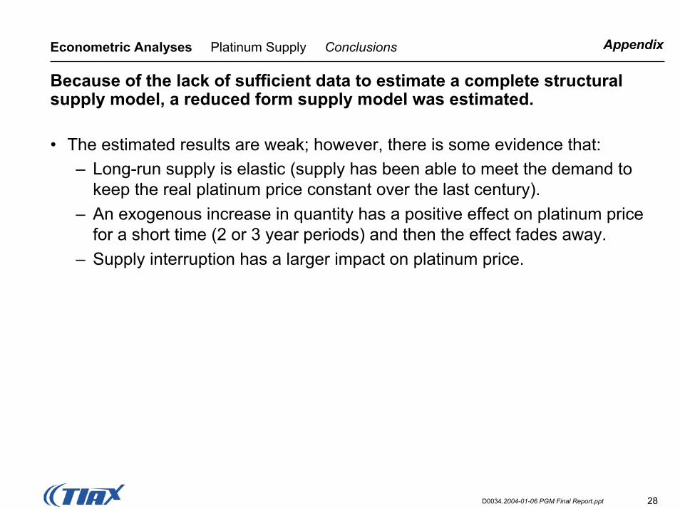
AppendixEconometric Analyses Platinum Supply Conclusions

Because of the lack of sufficient data to estimate a complete structural supply model, a reduced form supply model was estimated.

• The estimated results are weak; however, there is some evidence that:– Long-run supply is elastic (supply has been able to meet the demand to

keep the real platinum price constant over the last century).– An exogenous increase in quantity has a positive effect on platinum price

for a short time (2 or 3 year periods) and then the effect fades away.– Supply interruption has a larger impact on platinum price.


AppendixEconometric Analyses Equilibrium Displacement Simulation

We simulated the impact of FCV demand on platinum price, using the results from our econometric models, the price elasticity of platinum autocatalyst demand*, and hypothetical FCV demand. • The simulation model was specified as follows:

J OAS A J O

FCdP Q

Q QQPQ Q Qε η η η

= + + +

Q The elasticity of demand for Pt in automotive use*

Total quantity of Pt sold ηΑ

QAQ Share of automotive use of Pt

QJQ

QoQ

FCQ

ηj The elasticity of demand for Pt jewelry

Share of jewelry use of Pt

ηo The elasticity of demand for other useShare of other use of Pt

Hypothetical fraction of total Pt consumption by fuel cell use

εs Price elasticity of supply of Pt

This model is the fundamental link among all parts of the simulation model.* Obtained from a conceptual model of the general equilibrium derived demand. Derivation is available upon request.


AppendixEconometric Analyses Simulation Model

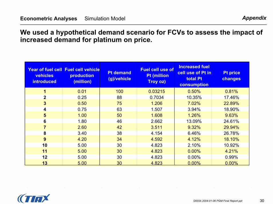
We used a hypothetical demand scenario for FCVs to assess the impact of increased demand for platinum on price.

Year of fuel cell vehicles

introduced

Fuel cell vehicle production

(million)

Pt demand (g)/vehicle

Fuel cell use of Pt (millionTroy oz)

Increased fuel cell use of Pt in

total Pt consumption

Pt price changes

1 0.01 100 0.03215 0.50% 0.81%2 0.25 88 0.7034 10.35% 17.46%3 0.50 75 1.206 7.02% 22.89%4 0.75 63 1.507 3.94% 18.90%5 1.00 50 1.608 1.26% 9.63%6 1.80 46 2.662 13.09% 24.61%7 2.60 42 3.511 9.32% 29.94%8 3.40 38 4.154 6.46% 26.78%9 4.20 34 4.592 4.12% 18.10%

10 5.00 30 4.823 2.10% 10.92%11 5.00 30 4.823 0.00% 4.21%12 5.00 30 4.823 0.00% 0.99%13 5.00 30 4.823 0.00% 0.00%


AppendixEconometric Analyses Simulation Model

The simulation illustrates that increased platinum demand will increase the price in the short-run, but in the long-run the price will return to its base level once supply catches up with demand.

0%

5%

10%

15%

20%

25%

30%

35%

0 2 4 6 8 10 12Year

Perc

ent C

hang

e fr

om In

itial

Yea

r

Initial increase in Pt demand from fuel cell vehicles

Price increases to respond to increased demand

Pt supply catches up to demand, price declines

More rapid growth in fuel cell vehicle production

Greater Pt price increase to respond to increased demand Pt supply catches up

to demand, price declines

Pt price returns to its base price

13

Fuel Cell Use of Platinum

Price Change

Simulation 2: Volatile Platinum DemandSimulation 2: Volatile Platinum Demand


AppendixEconometric Analyses Simulation Model Conclusions

The simulation model helps to highlight the following issues related to the impact of future FCV demand for platinum on price.

• Future demand for platinum from FCVs could drive up the price of platinum by 20 to 30 percent over its base price.

• A gradual adoption of fuel cell technology would minimize the pressure on platinum market and minimize the impact on platinum prices.

• Price declines over time are due to more elastic long-run supply and demand. The supply side has enough time to increase production and capacity and the demand side has the time to improve technology, to reduce platinum loading, or find alternatives.

Other factors outside the scope of our models could have an even more significant impact on platinum price than new FCV demand.• For example, even without demand from FCVs the 12/17/03 platinum price was

$840/oz (53% higher than the long-term mean) as a result of a supply/demand imbalance and other market factors.


AppendixAppendix



Vehicle Forecasts


Platinum Mining


AppendixVehicle Forecasts Vehicle Estimates

An increasing population in the US leads to increasing vehicle sales in a mature market.

0

5

10

15

20

25

30

35

1980 2000 2020 2040 2060

Veh

icle

Mar

ket (

mill

ion

unit

sale

s)

0

50

100

150

200

250

300

350

400

450

Tota

l Pop

ulat

ion

(mill

ions

)

Sources: United Nations, Ward’s, DOE Energy Information Administration* Vehicle Turnover Period = 15.5 years

0.67 veh/cap

0.83 veh/cap

0.84 veh/cap

Population

Vehicle Sales DOE Projection

Sales Forecast

US Vehicle MarketUS Vehicle Market



The Western European market is mature, but the rise in vehicle per capita ownership offsets the effect of a projected decrease in population.

Sources: United Nations, Ward’s, DOE Energy Information Administration* Vehicle Turnover Period = 11.5 years

0

5

10

15

20

25

1980 2000 2020 2040 2060

Veh

icle

Mar

ket (

mill

ion

unit

sale

s)

0

50

100

150

200

250

300

350

Tota

l Pop

ulat

ion

(mill

ions

)

0.5 veh/cap

0.6 veh/cap 0.7 veh/cap

Population

DOE Projection Sales Forecast

Vehicle Sales

Western Europe Vehicle MarketWestern Europe Vehicle Market



The Japanese market trend is similar to Western Europe in our vehicle sales estimate.

Sources: United Nations, Ward’s, DOE Energy Information Administration* Vehicle Turnover Period = 10 years

0

2

4

6

8

10

12

1980 2000 2020 2040 2060

Veh

icle

Mar

ket (

mill

ion

unit

sale

s)

0

20

40

60

80

100

120

140

Tota

l Pop

ulat

ion

(mill

ions

)

0.6 veh/cap

0.64 veh/cap

0.7 veh/cap

Population

DOE Projection Sales ForecastVehicle Sales

Japan Vehicle MarketJapan Vehicle Market



The Chinese market has the potential to surpass the United states assuming vehicles per capita continues to rise with increasing GDP.


0

5

10

15

20

25

30

35

40

45

50

1980 2000 2020 2040 2060

Veh

icle

Mar

ket (

mill

ion

unit

sale

s)

0

200

400

600

800

1,000

1,200

1,400

1,600

Tota

l Pop

ulat

ion

(mill

ions

)

US Vehicle Projection in 2050

0.1 veh/cap

0.25 veh/cap

0.50 veh/cap

DOE ProjectionSales Forecast

Vehicle Sales

Population

0.01 veh/cap

0.05 veh/cap

Sale

s Fo

reca

st

Sales F

oreca

st

China Vehicle MarketChina Vehicle Market



The combination of increasing population and increased vehicles per capita leads to potentially the largest vehicle markets in India.

India Vehicle MarketIndia Vehicle Market

0

5

10

15

20

25

30

35

40

45

50

1980 2000 2020 2040 2060

Veh

icle

Mar

ket (

mill

ion

unit

sale

s)

0

200

400

600

800

1,000

1,200

1,400

1,600

1,800

2,000

Tota

l Pop

ulat

ion

(mill

ions

)


US Vehicle Projection in 2050

0.10 veh/cap

0.15 veh/cap

0.25 veh/cap

DOE Projection Sales Forecast

Vehicle Sales

Population

0.01 veh/cap

0.05 veh/cap

Sale

s Fo

reca

st

Sales F

orec

ast


AppendixVehicle Forecasts Vehicle Estimates 50% Scenario

The 50% Scenario shows that the world vehicle fleet will significantly increase as Developing Countries increase their vehicles per capita.

0

200

400

600

800

1,000

1,200

1,400

2005 2010 2015 2020 2025 2030 2035 2040 2045 2050

Vehi

cle

Flee

t (m

illio

ns)

Total Selected Countries

United States

W. Europe

JapanChina, India

0

200

400

600

800

1,000

1,200

1,400

2005 2010 2015 2020 2025 2030 2035 2040 2045 2050

Veh

icle

Fle

et (m

illio

ns)


Selected Developing Countries

Selected Developed Countries

50% Scenario50% Scenario 50% Scenario50% Scenario

Sources: United Nations, Ward’s, DOE Energy Information Administration* Rest of world may add 20% to vehicle sales based on 2000 statistics


AppendixVehicle Forecasts Vehicle Estimates 80% Scenario

The 80% Scenario shows that the world vehicle fleet will significantly increase as Developing Countries increase their vehicles per capita.

0

200

400

600

800

1,000

1,200

1,400

2005 2010 2015 2020 2025 2030 2035 2040 2045 2050

Vehi

cle

Flee

t (m

illio

ns)


Selected Developed Countries

Selected Developing Countries

0

200

400

600

800

1,000

1,200

1,400

2005 2010 2015 2020 2025 2030 2035 2040 2045 2050

Vehi

cle

Flee

t (m

illion

s)


United States

W. Europe

JapanChina, India

80% Scenario80% Scenario 80% Scenario80% Scenario

Sources: United Nations, Ward’s, DOE Energy Information Administration* Rest of world may add 20% to vehicle sales based on 2000 statistics


AppendixAppendix

Previous Studies


Vehicle Forecasts


Platinum Mining


AppendixStationary Fuel Cell Markets Objective

We evaluated stationary global PEMFC markets for the scenario in which PEMFC achieves success in transportation applications.

Success Scenario

Stationary PEMFC cost and performance characteristics are consistent with the cost/performance needed for success in transportation applications.Achieving these cost performance characteristics will make PEMFC the distributed generation technology of choice in stationary applications for distributed generation plant capacities under 1 MW.


AppendixStationary Fuel Cell Markets Key Assumptions/Simplifications

We used several simplifying assumptions for a scenario-based evaluation of the future stationary PEMFC market through 2050.

Global projections of new additions of electric generation capacity (from the International Energy Agency), with some adjustments, are a reasonable proxy for the target market.IEA generation capacity projections can be extrapolated from 2030 to 2050 using global Gross Domestic Product projections.Consistent with findings from previous TIAX studies, the simple payback period of stationary PEMFC in the U.S. are reasonably representative of the simple payback period in most significant global markets.Energy-cost savings at the end-use site will be the primary motivation to install PEMFC. PEMFC distribution chain markups will be at the low end of markups typically seen in the HVAC and Appliance industries.


AppendixStationary Fuel Cell Markets Global Generation Capacity

The IEA projects global electric generation capacity to more than double by 2030.

1150

3397 3397

4408

5683

1011

1275

1474

0

1000

2000

3000

4000

5000

6000

7000

8000

1971 1999 2010 2020 2030

Glo

bal E

lect

ric G

ener

atio

n C

apac

ity, G

W

Net Capacity Additions

4408

5683

7157

3397

Source: World Energy Outlook 2002; International Energy Agency; pp. 411, 424-498.1971 installed base derived from EIA consumption data (5,250 TWh), and the 1999 Capacity Factor (0.52).



U.S./Canada, the European Union, and China combined account for about 50 percent of current and projected future generation capacity.

0

200

400

600

800

1,000

1,200

1,400

1,600

US and C

anad

aMex

ico

Europe

an U

nion

Other E

urope

Japa

n, Au

strali

a, New

Zeala

nd

Other P

acific

Rim

Russia

Other F

ormer

Soviet

China

East A

sia (in

cludin

g Ind

ones

ia)

South

Asia

(inclu

ding I

ndia)

Latin

Ameri

ca (in

lcudin

g Braz

il)Midd

le Eas

tAfr

ica

1999 Installed Base Capacity 2010 Aditional Net Capacity2020 Aditional Net Capacity 2030 Aditional Net Capacity

Elec

tric

Gen

erat

ion

Cap

acity

(GW

)

Source: World Energy Outlook 2002; International Energy Agency; pp. 424-498.



Projected total capacity additions include significant portions that will replace current aging assets.

Source: World Energy Outlook 2002; International Energy Agency; pp. 123-132, pp. 410-497, and Table 3.11.

3397

10111275 1474

147

250400

0

500

1000

1500

2000

2500

3000

3500

4000

1999 InstalledCapacity

2000-2010CapacityAdditions



Glo

bal E

lect

ric G

ener

atio

n C

apac

ity, G

W

Net Additions

Replacing Existing Assets


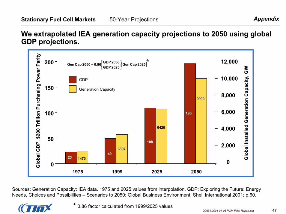
AppendixStationary Fuel Cell Markets 50-Year Projections

We extrapolated IEA generation capacity projections to 2050 using global GDP projections.

0

50

100

150

200

1975 1999 2025 2050

Glo

bal G

DP,

$20

0 Tr

illio

n Pu

rcha

sing

Pow

er P

arity

2349

108

196

0

2,000

4,000

6,000

8,000

10,000

12,000

Glo

bal I

nsta

lled

Gen

erat

ion

Cap

acity

, GW

1470

3397

6420

9990

[ ]2025 Cap Gen2025 GDP2050 GDP0.86 2050 Cap Gen

=

Sources: Generation Capacity: IEA data. 1975 and 2025 values from interpolation. GDP: Exploring the Future: Energy Needs, Choices and Possibilities – Scenarios to 2050; Global Business Environment, Shell International 2001; p.60.

GDP

Generation Capacity

*

* 0.86 factor calculated from 1999/2025 values


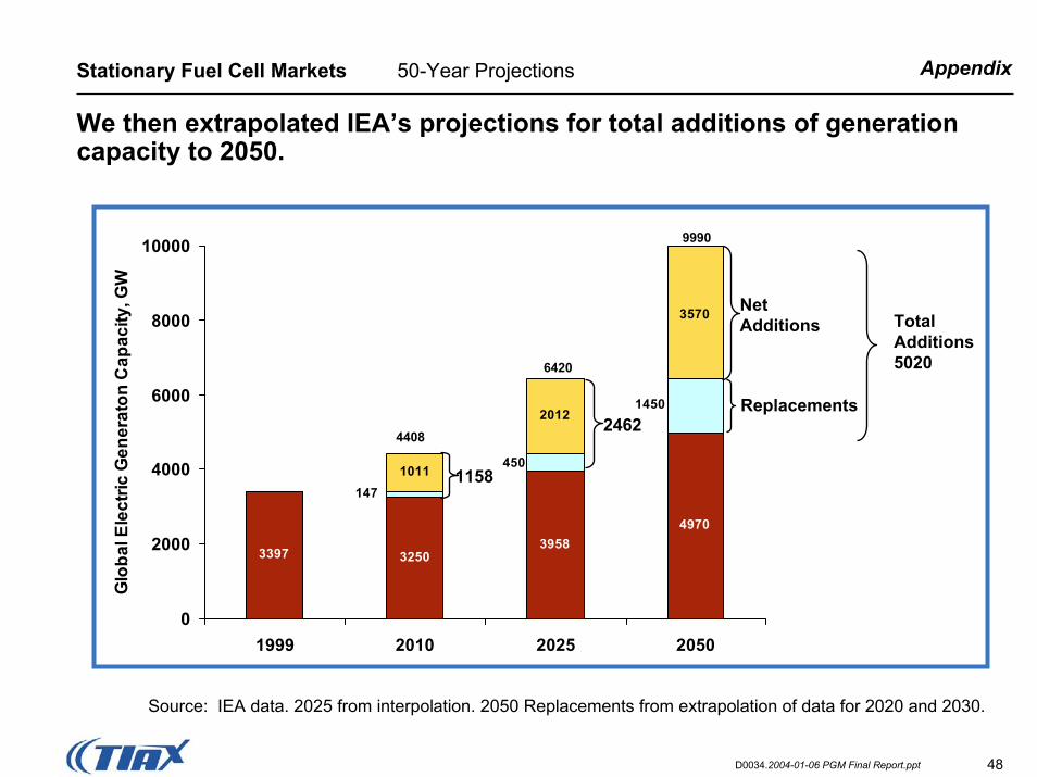
AppendixStationary Fuel Cell Markets 50-Year Projections

We then extrapolated IEA’s projections for total additions of generation capacity to 2050.

3397 32503958

4970

1450

450

147

3570

2012

1011

0

2000

4000

6000

8000

10000

1999 2010 2025 2050

Glo

bal E

lect

ric G

ener

aton

Cap

acity

, GW

Net Additions

1158

2462

Total Additions5020

4408

6420

9990

Replacements

Source: IEA data. 2025 from interpolation. 2050 Replacements from extrapolation of data for 2020 and 2030.


AppendixStationary Fuel Cell Markets Cost Analysis Stationary PEMFC Cost/Performance

Stationary PEMFC cost and performance characteristics were estimated from the requirements for a successful transportation PEMFC market.

System Cost

Efficiency

Requirements for a Successful Transportation MarketRequirements for a Successful Transportation Market

$50/kW

35% (LHV*)

* Lower Heating Value


AppendixStationary Fuel Cell Markets Cost Analysis Stationary PEMFC Performance

Net generation efficiency in stationary applications will be slightly higher than for transportation applications.

Transportation

35% (LHV)

Performance Projections

Stationary 2010+


Stationary 2025+

40% (LHV)

RationaleRationale

• Rated at 0.75 to 0.80 volts/cell for stationary applications, vs. 0.65 to 0.70 volts/cell for transportation, to optimize efficiency (rather than power density)

• This efficiency benefit is adjusted down slightly to account for power-conditioning losses associated with stationary PEMFC.

• We assumed the upper end of the efficiency range for stationary applications would be achieved.


AppendixStationary Fuel Cell Markets Cost Analysis Stationary PEMFC Manufactured Cost

The manufactured cost of stationary PEMFC will be 4 to 8 times the cost for transportation applications.

TransportationPerformance Projections

Stationary 2010+

$50/kW $400/kW


Stationary 2025+

$200/kWRated at 0.65 to 0.70 volts/cell Rated to 0.75 to 0.80 volts/cell

Rationale Rationale –– Additional Requirements for Stationary PEMFCAdditional Requirements for Stationary PEMFC

• Power conditioning subsystems to produce alternating current at the required voltage and frequency

• Utility interface subsystems (including electric grid interconnection)

• Packaging (the vehicle provides the packaging for transportation applications)

• More robust components (40,000 hour life required for major subsystems vs. 5,000 hours for transportation):– Higher catalyst loadings in fuel-cell stack– Thicker, more robust, membrane structures– More robust electromechanical equipment (pumps, blowers, valves, etc.)

• Different cell voltage rating to optimize efficiency (rather than power density)

• Fuel processor subsystem to operate on natural gas or other fossil fuel


AppendixStationary Fuel Cell Markets Cost Analysis Installed Cost

We estimated distribution chain markups based on the low end of mark-up ranges for appliances and HVAC equipment.

2010+: $400/kW

$200/kW+ 20 %

Factory Markup1

$480/kW

$240/kW

Factory Price

+ 75 %

Distributor & Installer Markups (traditional 2-step

distribution assumed)

$840/kW

$420/kW

Installed Cost2Manufactured Cost

2025+:

1 Low end of 20-40 percent range.2 Assumes straight forward installation and simple, standardized grid interconnection requirements.


AppendixStationary Fuel Cell Markets Cost Analysis

For this scenario, using TIAX analytical tools1, we estimate a simple payback period of about 8 years in 2010, improving to 4 years in 2025.

0

2

4

6

8

10

12

14

16

18

20

0.30 0.32 0.34 0.36 0.38 0.40 0.42 0.44 0.46 0.48 0.50

Net Generating Efficiency (LHV)

Sim

ple

Payb

ack

Perio

d (Y

ears

) Fort Worth Office Building $0.08/kWh Electricity (Fixed Rate)$5/MMBtu Natural GasCapacity Factor = 0.54$0.01/kWh Non-Fuel O&M

2010+: $840/kW Installed Cost

2025+: $420/ kW Installed Cost

Representative ApplicationRepresentative Application

1 Developed for the U.S. Department of Energy under UT-Battelle Subcontract No. 4000008858; completed April 12, 2002.


AppendixStationary Fuel Cell Markets Market Penetration

Simple payback period is often used as an initial screen of energy-saving technologies.

Simple Payback Period (Years)Simple Payback Period (Years)

• Defined as:

• Accounts for:– Installed Cost– Electricity Cost Savings– Fuel Cost– Non-Fuel O&M

• Does NOT Account for:– Cost of Capital– Product Life, Salvage Value, or Replacement Cost– Non-energy-saving Benefits

Savings Net AnnualCost Installed



TIAX has developed simplified relationships to predict market penetration based on payback period.

TIAX Market Penetration Curves for Residential and Commercial

BuildingsBased on field interviews, consumer surveys, and market data on adoption of efficient technologiesUseful as guidelines for market acceptance ratesGeneral observations:

threshold payback is 4-5 yrslarge market penetration occurs at <3 yrs

Market Penetration Curves for Efficient Technologies in

Commercial Buildings

Years to Payback

0

10

20

30

40

50

60

70

80

90

100

0 1 2 3 4 5 6 7 8 9 10

Ultimate Adoption(10–20 Years Following Introduction)

Five YearsFollowing Introduction

Perc

ent o

f Tar

get P

enet

ratio

nThird Party/Utility

Owner Occupied/Institutional

Lease/Rental

CustomerCustomer--Owned (Residential/Commercial) Owned (Residential/Commercial)

Sources: TIAX estimates, based on HVAC market penetration experience



We increased the resulting market penetrations to account for other factors, based on TIAX experience.

Time PeriodTime Period Installed CostInstalled Cost Simple PaybackSimple Payback Unadjusted Market Unadjusted Market PenetrationPenetration11

Adjusted Market Adjusted Market PenetrationPenetration22

2010+ $840/kW 8 years 2%3 3%

2025+ $420/kW 4 years 12%4 15%

Examples of Other FactorsExamples of Other Factors

Power quality/reliabilityFuel flexibilityEnergy securityAdditional savings from cogeneration in some applicationsTransmission and distribution system support

1) Based on energy-cost economics alone2) Includes Other Factors.3) Based on market penetration curve for “5 years following market introduction”.4) Based on market penetration curve for “ultimate adoption”.


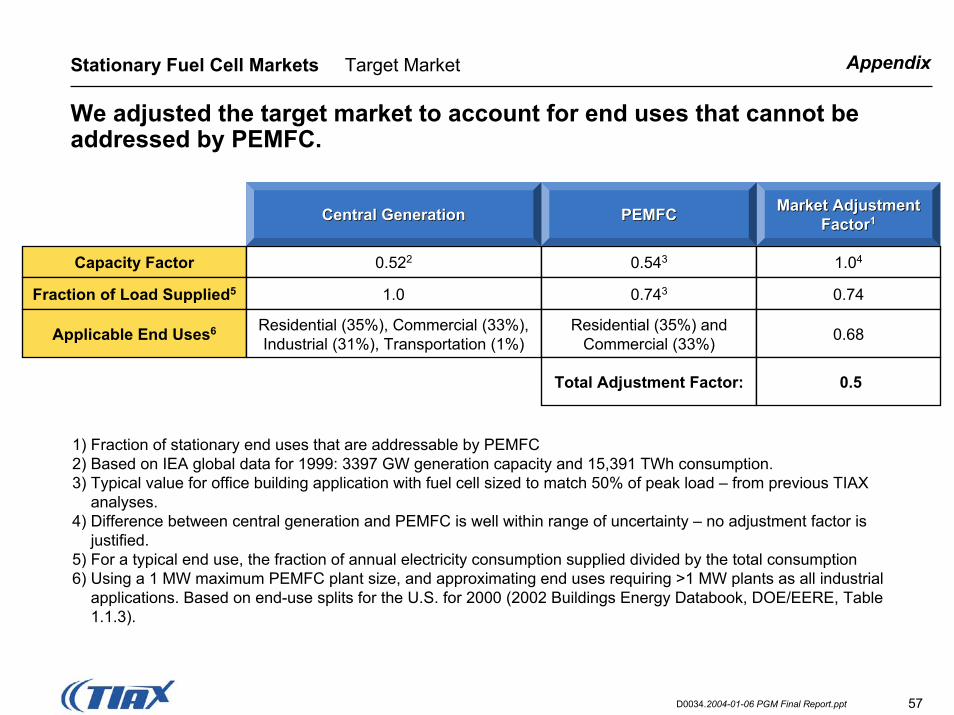
AppendixStationary Fuel Cell Markets Target Market

We adjusted the target market to account for end uses that cannot be addressed by PEMFC.

Capacity Factor 0.522 0.543 1.04

Fraction of Load Supplied5 1.0 0.743 0.74

Applicable End Uses6 Residential (35%), Commercial (33%),Industrial (31%), Transportation (1%)

Residential (35%) andCommercial (33%) 0.68

Market Adjustment Market Adjustment FactorFactor11PEMFCPEMFCCentral GenerationCentral Generation

Total Adjustment Factor: 0.5

1) Fraction of stationary end uses that are addressable by PEMFC2) Based on IEA global data for 1999: 3397 GW generation capacity and 15,391 TWh consumption.3) Typical value for office building application with fuel cell sized to match 50% of peak load – from previous TIAX

analyses.4) Difference between central generation and PEMFC is well within range of uncertainty – no adjustment factor is

justified.5) For a typical end use, the fraction of annual electricity consumption supplied divided by the total consumption6) Using a 1 MW maximum PEMFC plant size, and approximating end uses requiring >1 MW plants as all industrial

applications. Based on end-use splits for the U.S. for 2000 (2002 Buildings Energy Databook, DOE/EERE, Table 1.1.3).


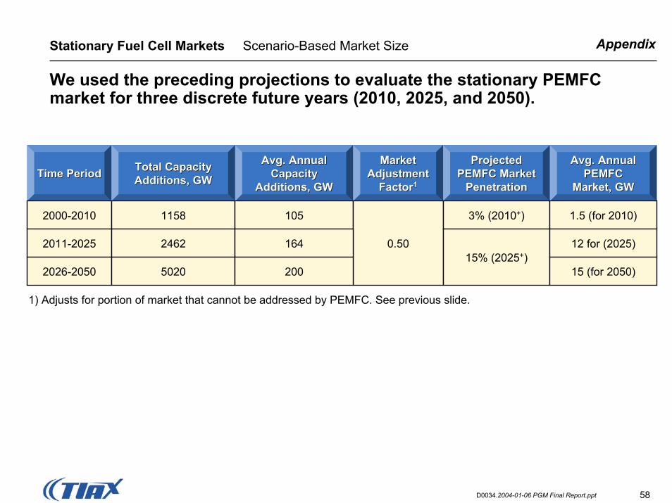
AppendixStationary Fuel Cell Markets Scenario-Based Market Size

We used the preceding projections to evaluate the stationary PEMFC market for three discrete future years (2010, 2025, and 2050).

Time PeriodTime Period Total Capacity Total Capacity Additions, GWAdditions, GW

Avg. Annual Avg. Annual Capacity Capacity

Additions, GWAdditions, GW

Market Market Adjustment Adjustment

FactorFactor11

Projected Projected PEMFC Market PEMFC Market

PenetrationPenetration

Avg. Annual Avg. Annual PEMFC PEMFC

Market, GWMarket, GW

2000-2010 1158 105 3% (2010+) 1.5 (for 2010)

2011-2025 2462 164 0.50 12 for (2025)15% (2025+)

2026-2050 5020 200 15 (for 2050)

1) Adjusts for portion of market that cannot be addressed by PEMFC. See previous slide.


AppendixStationary Fuel Cell Markets Market Projections

We generated a reasonable penetration curve based on the 2010, 2025, and 2050 market penetrations.

02468

10121416

2000 2010 2020 2030 2040 2050Year

Annu

al P

EMFC

Inst

alla

tions

, GW

New PEMFC installations only – Does not include stack

replacements for existing installations

X

X

X


AppendixAppendix



Vehicle Forecasts


Platinum Mining


AppendixPlatinum Mining Geological Information Introduction

PGMs are mined in only a few locations throughout the world, with more than 90% of platinum production concentrated in South Africa and Russia.

• PGMs are localized in mafic to basalatic magmatic complexes– Layered: Bushveld (South Africa),

Stillwater (United States), Great Dyke (Zimbabwe)

– Massive: Norlisk (Russia), Sudbury (Canada)- Associated with nickel-copper

deposits

• Placer deposits (alluvial)– Urals, Alaska

Layered deposits account for 75% of platinum production and resources and massive deposits account for the balance.


AppendixPlatinum Mining Geological Information Introduction

Platinum is one of six PGMs recovered along with base and precious metals.

• Platinum

• Palladium

• Rhodium

• Iridium

• Osmium

• Ruthenium

PGMsPGMs

Base Metals• Nickel

• Chromium

• Copper

Base Metals

Precious MetalsPrecious Metals

• Gold

• Silver


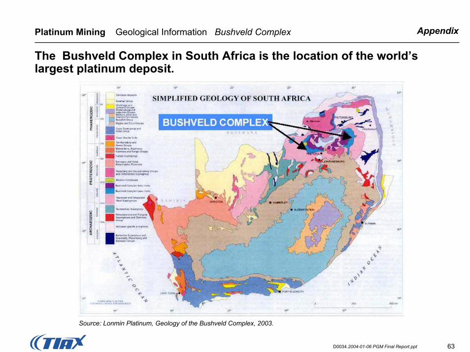
AppendixPlatinum Mining Geological Information Bushveld Complex

The Bushveld Complex in South Africa is the location of the world’s largest platinum deposit.

Source: Lonmin Platinum, Geology of the Bushveld Complex, 2003.



The Bushveld Complex contains an estimated 75% of the world’s platinum resources.

• The 3 most important PGM mineralized layers are:– Merensky Reef– UG2 Chromitite layer– Platreef

• Mafic portion of the complex is 2 billion years old

• PGM mineralization was discovered in 1924 on the eastern limb by Merenskyand Lombard.

• The Complex is the largest layered intrusion in the world:– Continuous over 300km– Aerial extent of over 65,000km2 (350 x 185km)– Depth of 7 to 9km



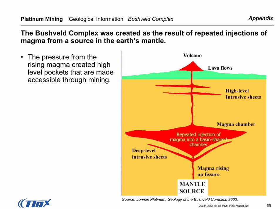
The Bushveld Complex was created as the result of repeated injections of magma from a source in the earth’s mantle.

• The pressure from the rising magma created high level pockets that are made accessible through mining.




The stratification of the mineral layers in the Bushveld Complex was created by the continual crystallization of magma from within the earth’s mantle.• Enormous volumes of magma

developed layers (stratification)

• Minerals crystallized as the temperature fell

• These minerals accumulated into sub-horizontal layers, building up from the base of the magma chamber

• Intermittent replenishment of the chamber by hotter magma led to a repetition of this crystallization sequence, leading to concentration of minerals in layers of chromititeand magnetite

MAFIC INTRUSION


This process led to a 1000 fold increase in PGM concentration.



The Bushveld geology is more complicated than the idealized layered deposit.

Idealized Platinum section

(Molengraaf—1905)

East–West section

(Meyer & De Beer—1954)


East–West section

(Du Toit—1954)



The Complex is divided into an Eastern and Western location

Source: Lonmin Platinum, Geology of the Bushveld Complex, 2003* For size comparison with Bushveld Complex

Montana, USA*



The Western Bushveld is more heavily developed than the Eastern limb. Open pit mining occurs at PR Rustenberg.




Within the layered deposits, concentration profiles vary depending on the local conditions during formation.


This data influences site selection and how each deposit is mined.


AppendixPlatinum Mining Geological Information Reef Compositions

Platinum dominates the valuable elements of the Merensky, UG2, and Platreef ores.

Percent of PGM and GoldPercent of PGM and GoldMerensky Reef

E&W LimbsUG2

Western LimbUG2

Eastern LimbParameter Platreef

Pt

Pd

Rh

Ru

Ir

Os

Au

55–59

25

3–4

6–8

0.8–1.3

0.5–1

4–5

46–52

23–27

7.5–8.5

8.5–16

2–3

1

0.6–1.5

39 44

39 44

7 2.7

9 3.3

4 0.9

1.5 0.8

0.9 4.9Source: Lonmin Platinum, Geology of the Bushveld Complex, 2003.* % = (Wmetal / (Σ WPGMs + WAu)) x 10

i0

W = Weight


AppendixPlatinum Mining Geological Information Reef Compositions

The composition of the ores varies across the Bushveld Complex.


ParameterParameter Merensky ReefMerensky Reef UG2UG2 PlatreefPlatreef

Rock Type

PGE Content

Ni Content

Cu Content

BMS Content

BMS Grain Size

PGM Grain Size

Pyroxenite

4–10 g/t

0.13%

0.08%

1–10%

Up to 10 mm

Up to 350 um

Density 3.2 g/cm2

Chromitite Pyroxenite

4–10 g/t 4–5 g/t

0.07% 0.36%

0.02% 0.18%

<1% N/A

30 um N/A

Up to 10 um N/A

4 g/cm2 N/A


Platinum Mining Geological Information Reef depth and mined areas in the SW Bushveld Appendix

Currently the shallower deposits, less than 1,000m, are being exploited.



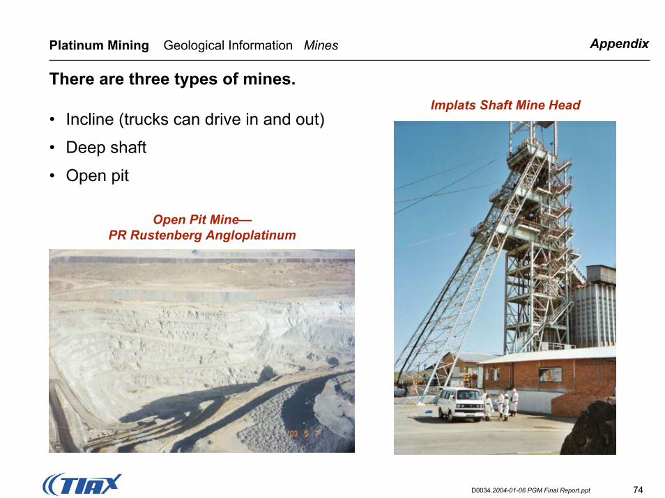
AppendixPlatinum Mining Geological Information Mines

There are three types of mines.Implats Shaft Mine Head

• Incline (trucks can drive in and out)

• Deep shaft

• Open pit

Open Pit Mine—PR Rustenberg Angloplatinum


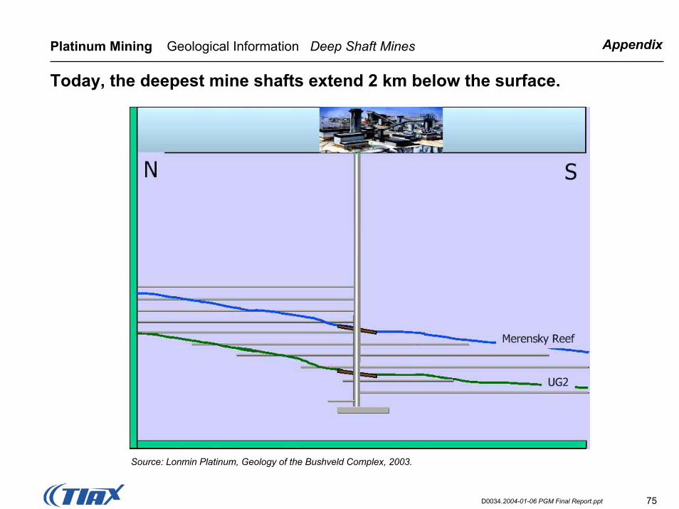
AppendixPlatinum Mining Geological Information Deep Shaft Mines

Today, the deepest mine shafts extend 2 km below the surface.



AppendixPlatinum Mining Geological Information Deep Shaft Mines

A network of shafts spread horizontally from the main shaft to gain access to PGM rich deposits.



AppendixPlatinum Mining Production Process Flow Chart

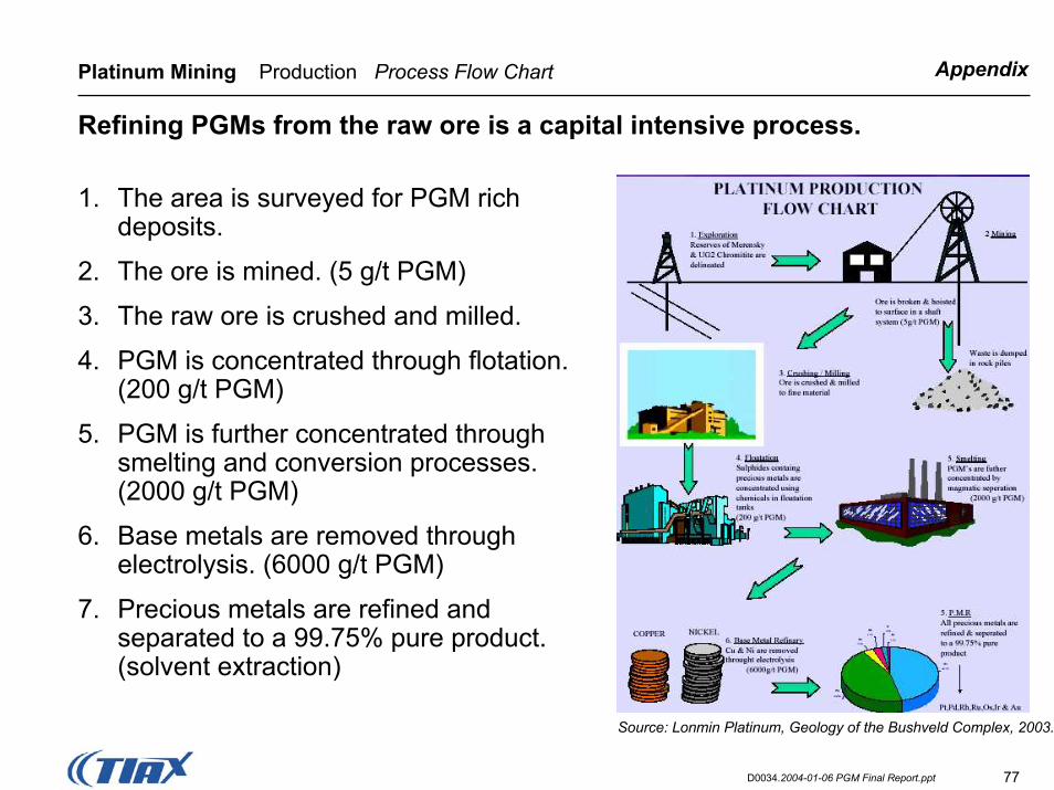
Refining PGMs from the raw ore is a capital intensive process.

1. The area is surveyed for PGM rich deposits.

2. The ore is mined. (5 g/t PGM)

3. The raw ore is crushed and milled.

4. PGM is concentrated through flotation. (200 g/t PGM)

5. PGM is further concentrated through smelting and conversion processes. (2000 g/t PGM)

6. Base metals are removed through electrolysis. (6000 g/t PGM)

7. Precious metals are refined and separated to a 99.75% pure product. (solvent extraction)



AppendixPlatinum Mining Production Surveying

Aerial magnetic surveys are used to located PGM rich locations.




Geological disturbances degrade recovery efficiency and uniformity of the deposits.


The impact of these disturbances is evident in this photo and magnetic survey.



Potholes are large, saucer shaped deformities that greatly distort the structure of the ore body and cause disruptions to the mining operations.




3D seismic surveys are conducted to map the layered structure of a region.




Drilling rigs are used to extract core samples from the ground in order to quantify PGM concentrations and actual deposit geology.

Drilling Ring

Core Samples



AppendixPlatinum Mining Production Deep Shaft Mine

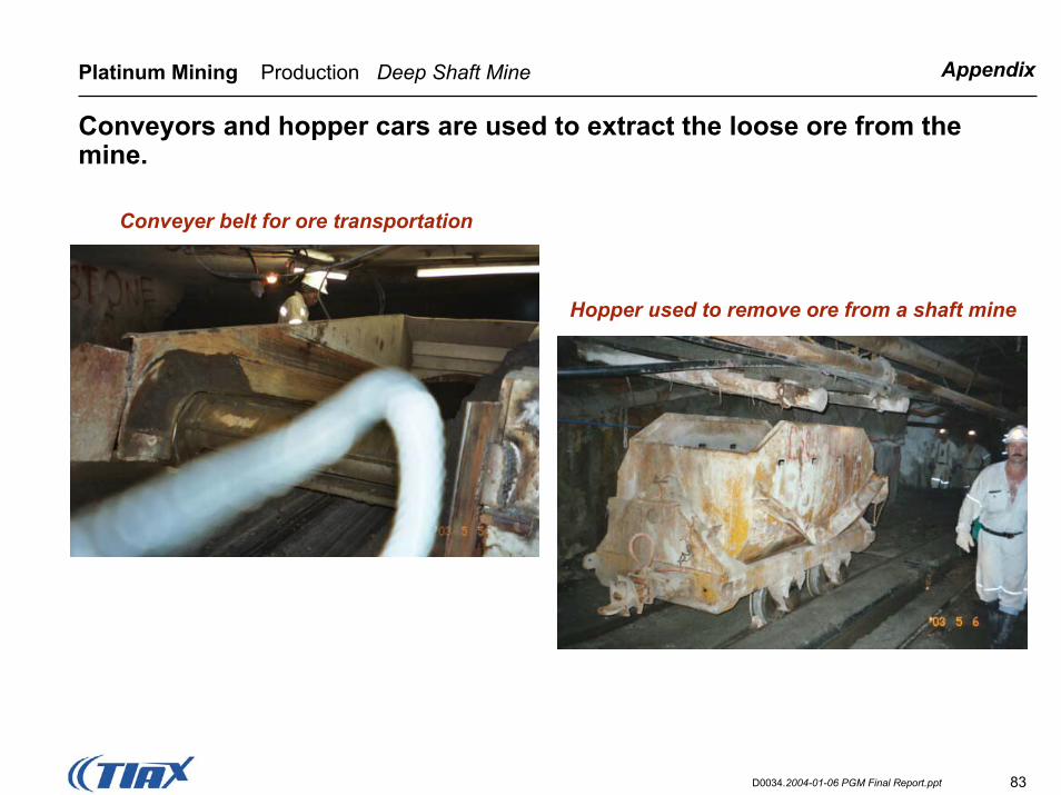
Conveyors and hopper cars are used to extract the loose ore from the mine.

Conveyer belt for ore transportation

Hopper used to remove ore from a shaft mine


AppendixPlatinum Mining Production Incline Mine

In an incline mine, workers can use mechanized drills to prepare the mine face for blasting.

Workers Drilling


AppendixPlatinum Mining Production Incline Mine

Mining technology is moving to reduce the height of equipment in order to reduce the amount of tailings that need to be processed.

Roof Anchor

Excavating Ore


AppendixPlatinum Mining Production

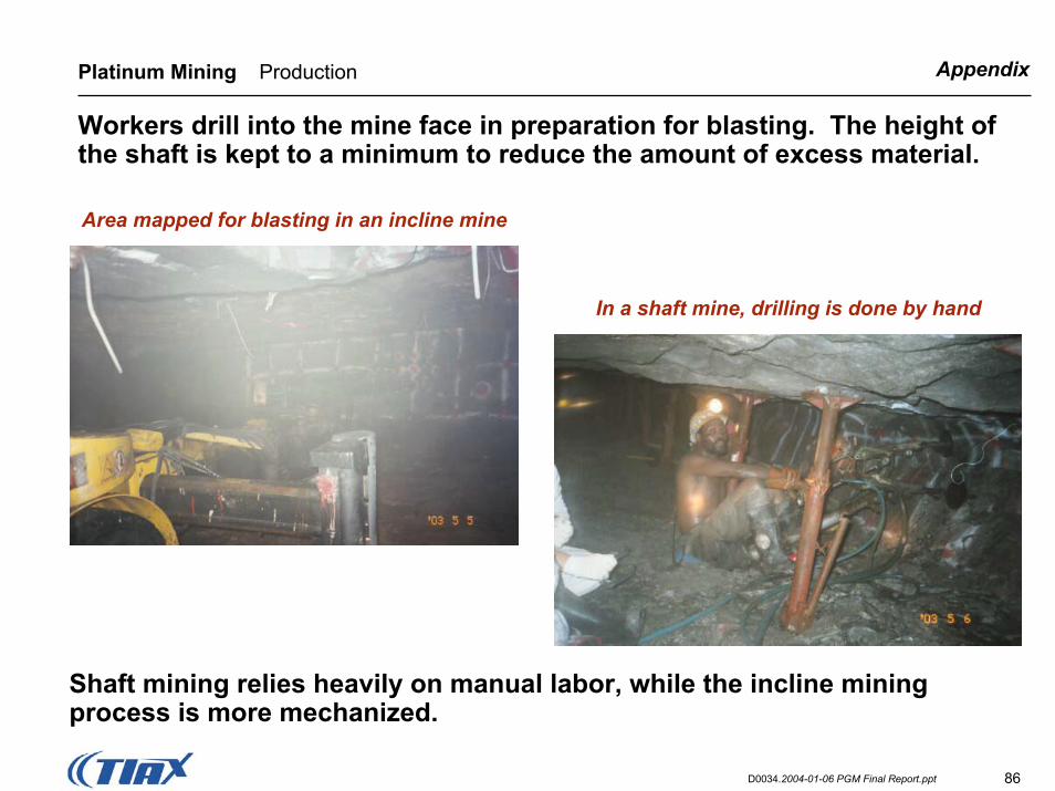
Workers drill into the mine face in preparation for blasting. The height of the shaft is kept to a minimum to reduce the amount of excess material.

Area mapped for blasting in an incline mine

In a shaft mine, drilling is done by hand

Shaft mining relies heavily on manual labor, while the incline mining process is more mechanized.


AppendixPlatinum Mining Production Open Pit Mine

In open pit mining, large quantities of material are removed to expose the valuable PGM layers.

Non-ore materialremoved to expose

the PGM layerPGM layer tobe processed



In open pit mining, large quantities of material are removed to expose the valuable PGM layers. (continued)

Formation of a New Pit

Removal of Non-Ore

PGM face



Sophisticated controls are used to monitor material flow, traffic, and the condition of the equipment.

Truck Used to Haul Ore

Monitoring Station


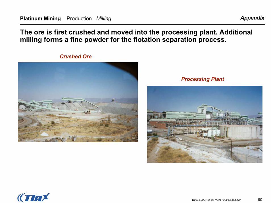
AppendixPlatinum Mining Production Milling

The ore is first crushed and moved into the processing plant. Additional milling forms a fine powder for the flotation separation process.

Crushed Ore

Processing Plant


AppendixPlatinum Mining Production Flotation

The powder is then moved through a series of flotation tanks.

• The powder is mixed with water and special reagents.

• Air is pumped through the mixture, causing a PGM rich matte to float to the surface.

• The matte rises over the rim of the tank and flows to the next floatation tank.

• The process continues through several more tanks, each increasing the PGM concentration.



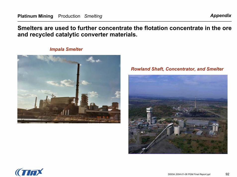
AppendixPlatinum Mining Production Smelting

Smelters are used to further concentrate the flotation concentrate in the ore and recycled catalytic converter materials.

Impala Smelter

Rowland Shaft, Concentrator, and Smelter


AppendixPlatinum Mining Production Smelting

The material is smelted in an electric furnace at temperatures over 1500ºC.

Tapping the smelter

Filling a ladle to transport to the converters


AppendixPlatinum Mining Production Converting

Material is loaded into the converters where air is periodically blown through the molten material to remove the iron and sulfur.

Converters Cooling the converters


AppendixPlatinum Mining Production Base and Precious Metal Refining

The final two stages of the process involve separation of the metals.

• At the base metals refinery, the base metals are removed using electrolysis techniques.

• The PGMs are refined through a combination of solvent extraction, distillation, and ion exchange techniques.– Processes are proprietary.


AppendixPlatinum Mining Production Water Treatment

Water used in the refining process is treated and reused, as it is a precious commodity in South Africa.

Wastewater Treatment Plant


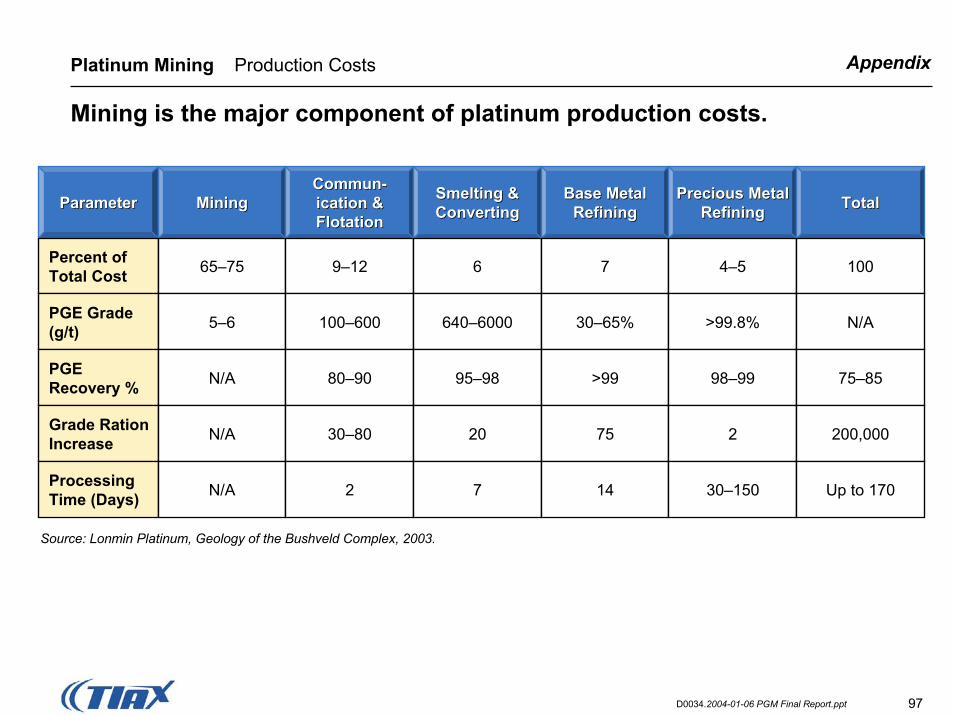
AppendixPlatinum Mining Production Costs

Mining is the major component of platinum production costs.


ParameterParameter MiningMining

Percent of Total Cost

PGE Grade (g/t)

PGE Recovery %

Grade Ration Increase

Processing Time (Days)

65–75

5–6

N/A

N/A

N/A

CommunCommun--ication & ication & FlotationFlotation

9–12

100–600

80–90

30–80

2

Smelting & Smelting & ConvertingConverting

6

640–6000

95–98

20

7

Base Metal Base Metal RefiningRefining

Precious Metal Precious Metal Refining

7

30–65%

>99

75

14

Refining Total

4–5

Total

100

>99.8% N/A

98–99 75–85

2 200,000

30–150 Up to 170

1 executive summary 2 project overview 3 platinum market ... · d0034.2004-01-06 pgm final...

Documents