11

Drought Monitoring over the United Drought Monitoring over the United StatesStates

Kingtse Mo Kingtse Mo

Climate Prediction CtClimate Prediction Ct

NCEP/NWS/NOAANCEP/NWS/NOAA

22

Our GoalsOur Goals

Provide users timely information and analysis Provide users timely information and analysis on drought. on drought.

Monitor atmospheric and hydrological Monitor atmospheric and hydrological conditions in support of operational Drought conditions in support of operational Drought Monitor and Drought OutlookMonitor and Drought Outlook

Develop regional applications in support of the NIDIS pilot project

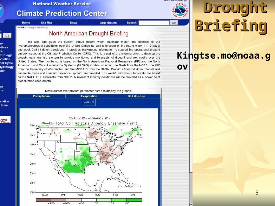
http://www.cpc.ncep.noaa.gov/products/Drought

33

Drought Drought Briefing Briefing

Kingtse.mo@noaa.gov

44

Current status Current status http://www.cpc.ncep.noaa.gov/products/Drought

Current conditions:Current conditions: Surface conditions ,drought indicesSurface conditions ,drought indices, E, P soil , E, P soil

moisture – from the ensemble NLDAS ( VIC, MOSAIC, moisture – from the ensemble NLDAS ( VIC, MOSAIC, SAC and VIC)SAC and VIC)

Atmospheric conditions and budget terms : NARRAtmospheric conditions and budget terms : NARR Forecasts: Forecasts:

U. Washington (ESP)U. Washington (ESP) Princeton U-EMC (downscaling from the CFS using Princeton U-EMC (downscaling from the CFS using

VIC)VIC) NSIPP (from NSIPP model)NSIPP (from NSIPP model)

55

Define drought based on the drought Define drought based on the drought IndicesIndices

Meteorological droughtMeteorological drought: : Precipitation deficit. Precipitation deficit. IndexIndex: : Standardized Precipitation IndexStandardized Precipitation Index Hydrological droughtHydrological drought: Streamflow or runoff deficit: Streamflow or runoff deficit Index:Index: Standardized runoff indexStandardized runoff index Agricultural droughtAgricultural drought: Total soil water storage deficit : Total soil water storage deficit IndexIndex: : SM anomaly percentileSM anomaly percentile

66

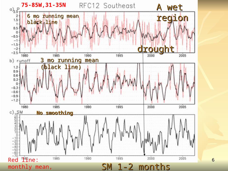
A wet regionA wet region

droughtdrought

6 mo running mean black line6 mo running mean black line

3 mo running mean (black line)3 mo running mean (black line)

SM 1-2 months delaySM 1-2 months delay

No smoothing No smoothing

Red line: monthly mean, no smoothing

75-85W,31-35N

77SM has much lower freq. over the western regionSM has much lower freq. over the western region

A dry regionUtah-AZ

88

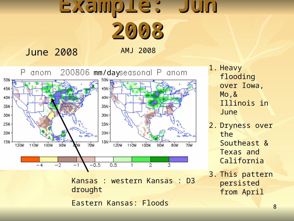
Example: Jun 2008Example: Jun 2008

1. Heavy flooding over Iowa, Mo,& Illinois in June

2. Dryness over the Southeast & Texas and California

3. This pattern persisted from April

June 2008 AMJ 2008

Kansas : western Kansas : D3 drought

Eastern Kansas: Floods

mm/day

99

1. Rainfall over the Mississippi basin influenced all SPI indices.

2. Dry: Southeast, southern Texas and California

3. Wet: Central U. S. and the upper Missouri basin (RFC 2 area)

Meteorological drought

D3 D2 D1 D0

1010

Hydrological DroughtHydrological Drought

Western Kansas Dry,

Eastern Kansas Wet

1111

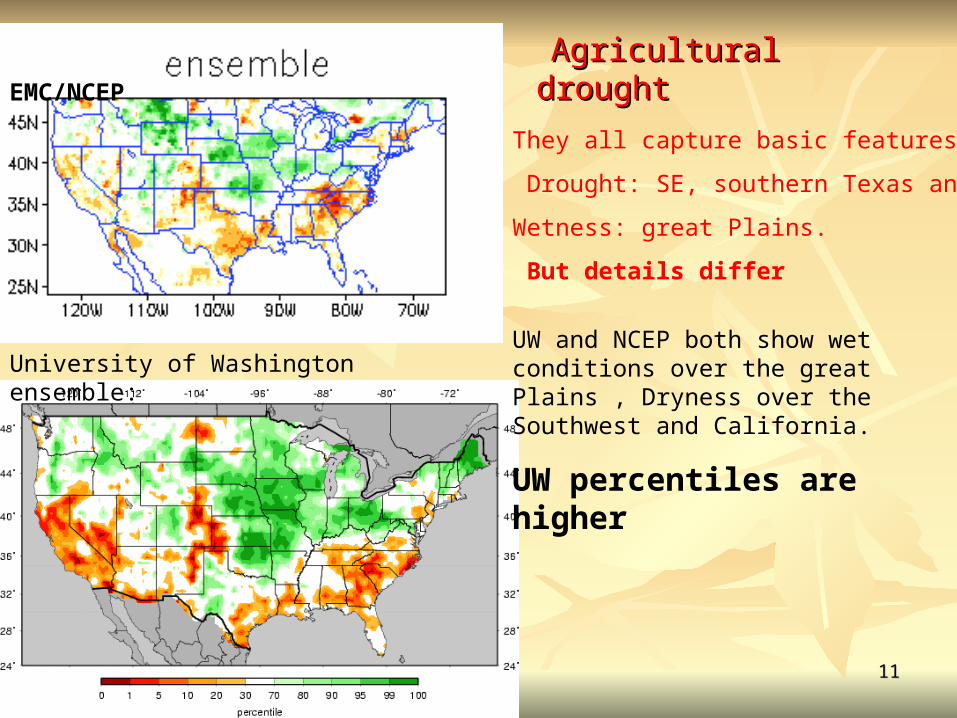
Agricultural droughtAgricultural drought

University of Washington ensemble:

They all capture basic features:

Drought: SE, southern Texas and California

Wetness: great Plains.

But details differ

UW and NCEP both show wet conditions over the great Plains , Dryness over the Southwest and California.

UW percentiles are higher

EMC/NCEP

1212

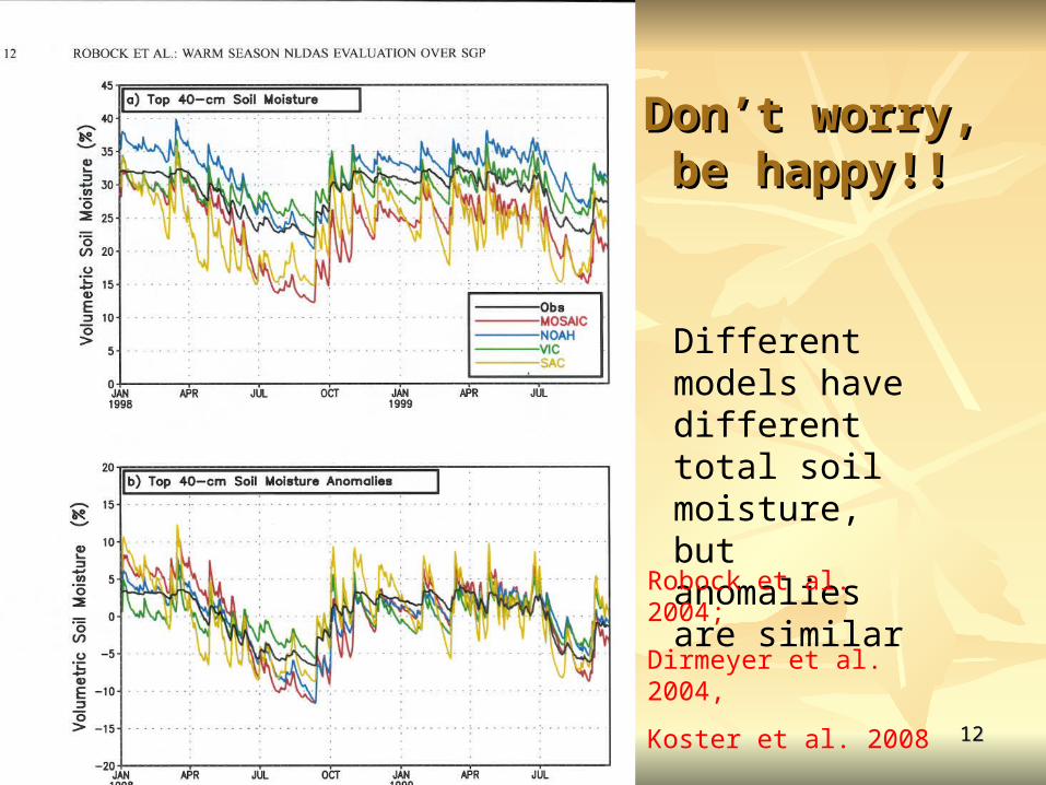
Don’t worry, be Don’t worry, be happy!!happy!!

Different models have different total soil moisture, but anomalies are similar

Robock et al. 2004;

Dirmeyer et al. 2004,

Koster et al. 2008

1313

ContributorsContributors

University of WashingtonUniversity of Washington Dennis Lettenmaier, Ted Bohn and Dennis Lettenmaier, Ted Bohn and

Shraddhanad ShuklaShraddhanad Shukla

EMCEMC EMC: Youlong Xia, Ken Mitchell & Mike EkEMC: Youlong Xia, Ken Mitchell & Mike Ek

1414

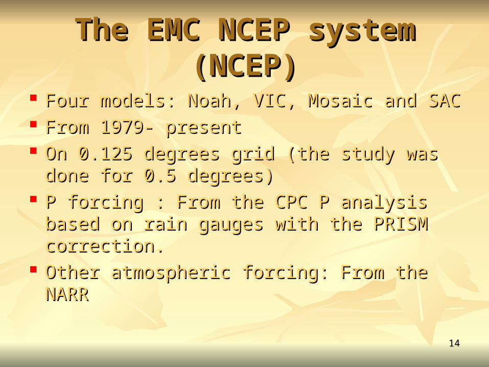
The EMC NCEP system (NCEP)The EMC NCEP system (NCEP)

Four models: Noah, VIC, Mosaic and SACFour models: Noah, VIC, Mosaic and SAC From 1979- presentFrom 1979- present On 0.125 degrees grid (the study was done for On 0.125 degrees grid (the study was done for

0.5 degrees)0.5 degrees) P forcing : From the CPC P analysis based on P forcing : From the CPC P analysis based on

rain gauges with the PRISM correction. rain gauges with the PRISM correction. Other atmospheric forcing: From the NARROther atmospheric forcing: From the NARR

1515

The University of Washington The University of Washington System (UW)System (UW)

Four models: Noah, VIC, SAC and CLMFour models: Noah, VIC, SAC and CLM From 1915-presentFrom 1915-present On 0.5 degrees gridOn 0.5 degrees grid P, Tsurf and low level winds from P, Tsurf and low level winds from

NOAA/NCDC co-op stationsNOAA/NCDC co-op stations No diurnal cycle in P, solar radiation was No diurnal cycle in P, solar radiation was

computed from Tsurfcomputed from Tsurf

1616

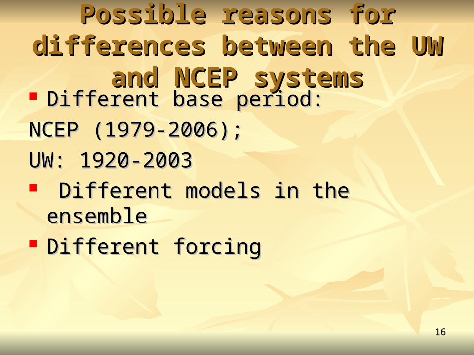
Possible reasons for differences Possible reasons for differences between the UW and NCEP systemsbetween the UW and NCEP systems

Different base period: Different base period:

NCEP (1979-2006);NCEP (1979-2006);

UW: 1920-2003 UW: 1920-2003 Different models in the ensembleDifferent models in the ensemble Different forcingDifferent forcing

1717

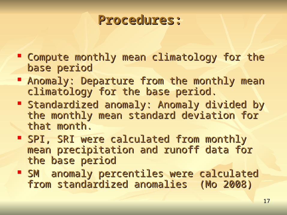
Procedures: Procedures:

Compute monthly mean climatology for the base period Compute monthly mean climatology for the base period Anomaly: Departure from the monthly mean Anomaly: Departure from the monthly mean

climatology for the base period.climatology for the base period. Standardized anomaly: Anomaly divided by the Standardized anomaly: Anomaly divided by the

monthly mean standard deviation for that month.monthly mean standard deviation for that month. SPI, SRI were calculated from monthly mean SPI, SRI were calculated from monthly mean

precipitation and runoff data for the base periodprecipitation and runoff data for the base period SM anomaly percentiles were calculated from SM anomaly percentiles were calculated from

standardized anomalies (Mo 2008)standardized anomalies (Mo 2008)

1818

Differences due to the base periodDifferences due to the base period

The UW system was used to study the impact of base The UW system was used to study the impact of base periods because their data cover 1915-2007.periods because their data cover 1915-2007.

SM %, SRI and SPI were computed for the period SM %, SRI and SPI were computed for the period 1979-2007 using the base period 1920-2007 and 1979-2007 using the base period 1920-2007 and 1979-2007 respectively.1979-2007 respectively.

RMS difference between SM % ( SRI or SPI) from RMS difference between SM % ( SRI or SPI) from the two base periods was computed for each modelthe two base periods was computed for each model

Same calculations were performed for the ensemble Same calculations were performed for the ensemble means (equally weighted mean)means (equally weighted mean)

1919

RMS diff of sm anomaly % for two base periods

Differences are small (less than 10%) except for the CLM model.

Noah

VIC

SAC

CLM

2020

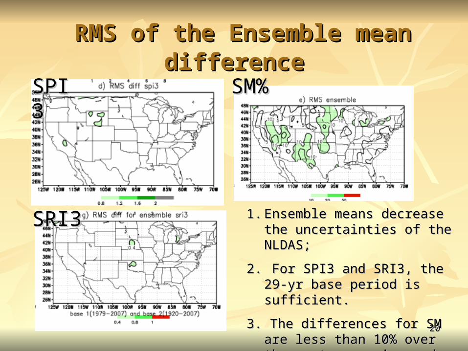
RMS of the Ensemble mean differenceRMS of the Ensemble mean difference

SPI3SPI3

SRI3SRI3

SM%SM%

1.1. Ensemble means decrease Ensemble means decrease the uncertainties of the the uncertainties of the NLDAS;NLDAS;

2.2. For SPI3 and SRI3, the 29-yr For SPI3 and SRI3, the 29-yr base period is sufficient.base period is sufficient.

3. The differences for SM are 3. The differences for SM are less than 10% over the less than 10% over the eastern region and about 10-eastern region and about 10-15 % over the western 15 % over the western interior regioninterior region

2121

Differences due to base periodDifferences due to base period

Ensemble mean decreases uncertainties and the RMS Ensemble mean decreases uncertainties and the RMS differences between two periods.differences between two periods.

For ensemble means, the 30-yr period is sufficient for For ensemble means, the 30-yr period is sufficient for SPI or SRI 3 months or longer.SPI or SRI 3 months or longer.

For SM %, the differences are less than 10% over the For SM %, the differences are less than 10% over the eastern United States, and 10~ 15% over the western eastern United States, and 10~ 15% over the western U. S.U. S.

If sudden changes occur, then outputs need to be If sudden changes occur, then outputs need to be calibrated before and after the change separately. calibrated before and after the change separately.

2222

mean SM percentiles and standardized anomalies for area 38-42N,110-115W

Black: monthly mean P wrt base (1920-2006);

Red: 6-mo running mean

The VIC has larger high frequency components. There were enough large positive/negative values before & after 1979 to make the percentiles similar for both base periods.

The CLM picks up the low freq. component

2323

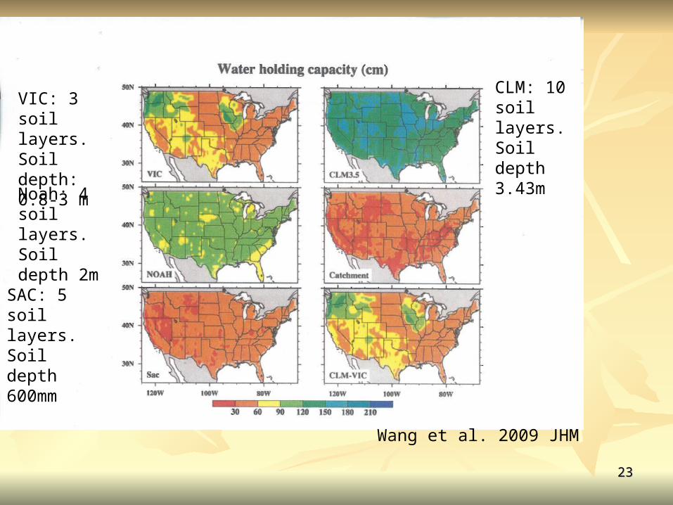
Wang et al. 2009 JHM

VIC: 3 soil layers. Soil depth: 0.8-3 m

Noah: 4 soil layers. Soil depth 2m

SAC: 5 soil layers. Soil depth 600mm

CLM: 10 soil layers. Soil depth 3.43m

2424

Measure the differences among models Measure the differences among models

Rm for a group of models m :the mean intermodel variance (or spread) int (m): interannual variance of the ensemble mean

)(int mR mm

Similar formula was used by Dirmeyer et al (2004). to assess Global wetness products except we use variance instead of standard dev.

2525

Differences due to forcingDifferences due to forcing

Differences are measured by R which is the Differences are measured by R which is the ratio between spread and interannual ratio between spread and interannual variability variability

R was calculated for the NCEP (4 models), the R was calculated for the NCEP (4 models), the UW (4 models) separately and two systems (8 UW (4 models) separately and two systems (8 models) pooled together for 1979-2007.models) pooled together for 1979-2007.

We computed R for SMWe computed R for SM

2626

R values for SM %R values for SM %1.1.The spread among the The spread among the

members from the members from the same system (UW or same system (UW or NCEP) is small. It is NCEP) is small. It is less than 0.4. (Fig. a less than 0.4. (Fig. a and b)and b)

2. R values with all UW 2. R values with all UW and NCEP members and NCEP members together is much larger together is much larger (Fig.c).(Fig.c).

This implies that the This implies that the mean differences mean differences between two systems between two systems are large are large

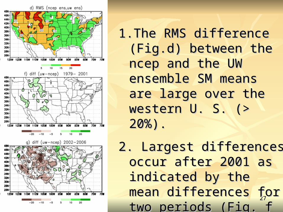
2727

1.1.The RMS difference The RMS difference (Fig.d) between the ncep (Fig.d) between the ncep and the UW ensemble and the UW ensemble SM means are large over SM means are large over the western U. S. (> the western U. S. (> 20%).20%).

2.2. Largest differences Largest differences occur after 2001 as occur after 2001 as indicated by the mean indicated by the mean differences for two differences for two periods (Fig. f and g)periods (Fig. f and g)

2828

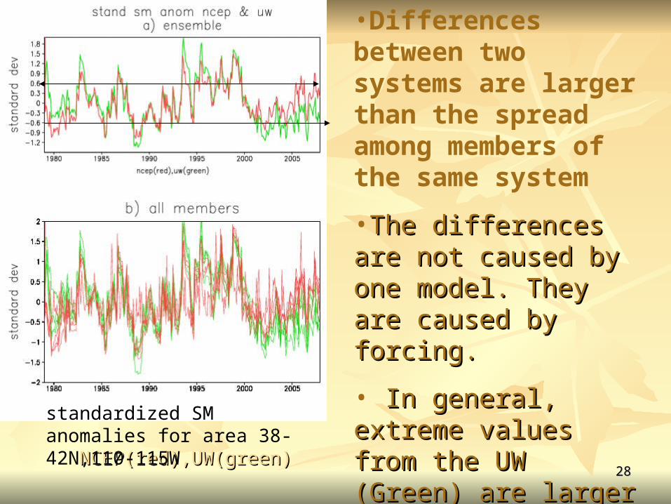
•Differences between two systems are larger than the spread among members of the same system

•The differences are The differences are not caused by one not caused by one model. They are model. They are caused by forcing.caused by forcing.

• In general, extreme In general, extreme values from the UW values from the UW (Green) are larger (Green) are larger than from the NCEP than from the NCEP (red) (red)

NCEP(red),UW(green)NCEP(red),UW(green)

standardized SM anomalies for area 38-42N,110-115W

2929

P and Tsurf differences are larger after 2002 P and Tsurf differences are larger after 2002 when systems went to operation in real timewhen systems went to operation in real time

There were less There were less station data after station data after 2002 when systems 2002 when systems went to real time went to real time operation. operation.

There are larger There are larger uncertainties in uncertainties in forcing forcing

The NCEP has The NCEP has larger P variances larger P variances than the UWthan the UW , so extreme values have smaller %.

3030

Uncertainties from different systemsUncertainties from different systems

Differences between members of the same system Differences between members of the same system (ncep or uw) are small. (runoff shows the same thing)(ncep or uw) are small. (runoff shows the same thing)

There are large differences between the NCEP and There are large differences between the NCEP and the UW systems. They are caused by forcing.the UW systems. They are caused by forcing.

Differences for historical period (before 2001 or Differences for historical period (before 2001 or 2002) were small. After systems went to operation in 2002) were small. After systems went to operation in near real time, station obs dropped and large near real time, station obs dropped and large differences occurred.differences occurred.

Currently, both systems will declare drought (wet Currently, both systems will declare drought (wet spells) , but they are likely to give different D spells) , but they are likely to give different D categories categories

3131

Model differencesModel differences

Characteristic time To– time scale of SM.Characteristic time To– time scale of SM. Correlations between different variables Correlations between different variables

For the common period 1979-2006 on 0.5 For the common period 1979-2006 on 0.5 resolution gridresolution grid

3232

Characteristic time :ToCharacteristic time :To

N

i

iRNiT1

0 )()/1(21

R(i) : auto correlation at time lag i, n=30

• To is calculated for each model and for the ensemble means.

• We also ask the question whether the spectral for SM is red. R(1) was computed for the NCEP ensemble mean. To was calculated for red noise model based on R(1) Delworth and Manabe 1988

Trenberth 1984

3333

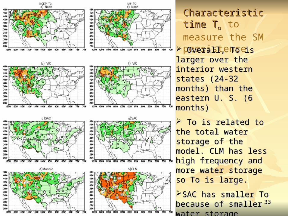
Characteristic time Characteristic time TTo o to measure the SM persistence

Overall, To is larger Overall, To is larger over the interior over the interior western states (24-32 western states (24-32 months) than the months) than the eastern U. S. (6 eastern U. S. (6 months) months)

To is related to the To is related to the total water storage of total water storage of the model. CLM has less the model. CLM has less high frequency and high frequency and more water storage so more water storage so To is large.To is large.

SAC has smaller To SAC has smaller To because of smaller because of smaller water storage water storage

3434

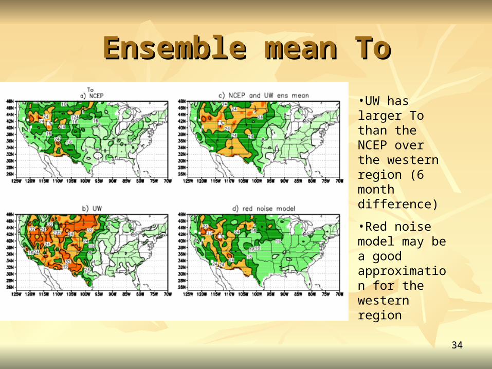
Ensemble mean ToEnsemble mean To

•UW has larger To than the NCEP over the western region (6 month difference)

•Red noise model may be a good approximation for the western region

3535

RunoffPEdt

dw

W= total Soil moistureW= total Soil moisture

PE

E

Soil moisture balance EqSoil moisture balance Eq

PE-potential evaporation= E when the PE-potential evaporation= E when the soil is sufficiently saturatedsoil is sufficiently saturated

Beta= evaporation efficiencyBeta= evaporation efficiency

RunoffPPEdt

dw )(

Beta is roughly proportional to W. If P-runoff is small,, then we can use red noise model

3636

Persistence of SM Measured by ToPersistence of SM Measured by To

To is larger over the interior western region To is larger over the interior western region (about 24-32 months) and smaller over the (about 24-32 months) and smaller over the eastern region (6 months). Therefore, drought eastern region (6 months). Therefore, drought over the western region tends to persist.over the western region tends to persist.

To from the UW is larger than the NCEP. To from the UW is larger than the NCEP. To is related to the water storage capacity of To is related to the water storage capacity of

the model.the model. Red noise model fits well for SM over the Red noise model fits well for SM over the

western region when P.-runoff is small western region when P.-runoff is small

3737

Relationships among variablesRelationships among variables

Tsurf and P are forcing for the NLAS. How do Tsurf and P are forcing for the NLAS. How do they relate to SM?they relate to SM?

Are there any direct (linear) relation between Are there any direct (linear) relation between them?them?

We study them using correlations. We study them using correlations.

3838

Correlations (Tsurf and SM) Correlations (Tsurf and SM) for ensemble meansfor ensemble means

No significant correlations for JFM, OND

The UW has weaker correlation between Tsurf and SM over the northern plains.

3939

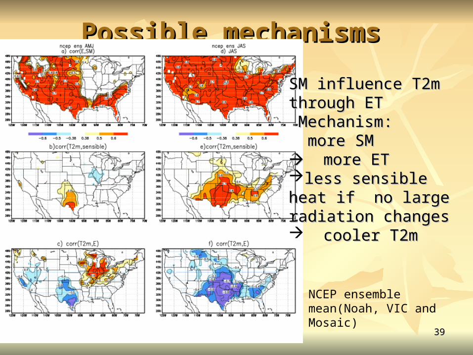
Possible mechanismsPossible mechanisms

NCEP ensemble mean(Noah, VIC and Mosaic)

SM influence T2m SM influence T2m through ETthrough ET Mechanism:Mechanism: more SM more SM more ETmore ETless sensible heat if no less sensible heat if no large radiation changeslarge radiation changes cooler T2mcooler T2m

4040

Possible mechanismsPossible mechanisms E is small in winter JFM and OND so no correlation between SM and Tsurf. E is small in winter JFM and OND so no correlation between SM and Tsurf. For AMJ, the Northeast is cold. For AMJ, the Northeast is cold. Warmer T2m => more vegetationWarmer T2m => more vegetation more transpirationmore transpiration so T2m and E are correlated. SM does not play a role.so T2m and E are correlated. SM does not play a role. For JAS, SM feedbacks to E so correlations are highFor JAS, SM feedbacks to E so correlations are high The UW has lower correlations over the northern plains. The UW has lower correlations over the northern plains.

4141

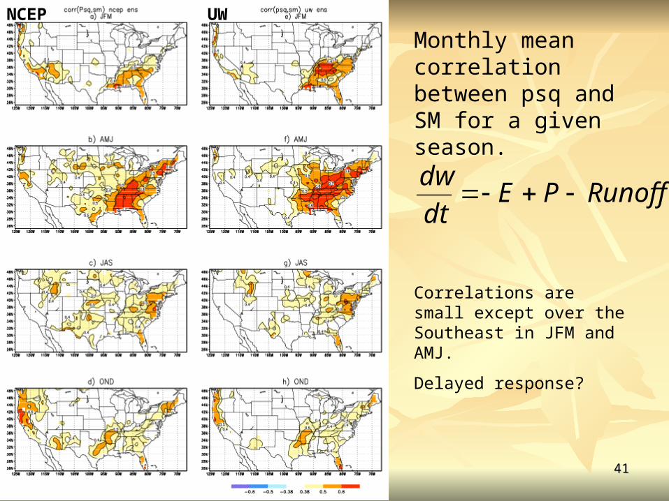
Monthly mean correlation between psq and SM for a given season.

NCEP UW

RunoffPEdt

dw

Correlations are small except over the Southeast in JFM and AMJ.

Delayed response?

4242

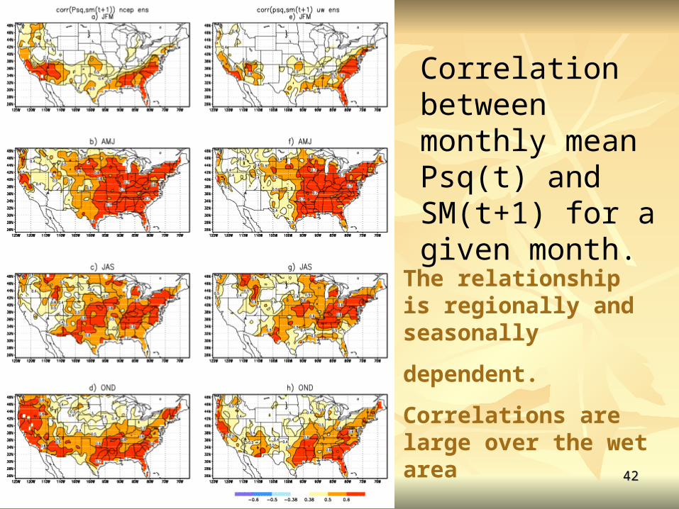
Correlation between monthly mean Psq(t) and SM(t+1) for a given month.

The relationship is regionally and seasonally

dependent.

Correlations are large over the wet area

4343

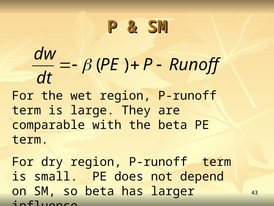
P & SMP & SM

For the wet region, P-runoff term is large. They are comparable with the beta PE term.

For dry region, P-runoff term is small. PE does not depend on SM, so beta has larger influence

RunoffPPEdt

dw )(

4444

Current drought conditions & Current drought conditions & outlookoutlook

4545

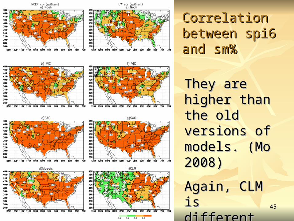
Correlation Correlation between spi6 between spi6 and sm%and sm%

They are They are higher than higher than the old the old versions of versions of models. (Mo models. (Mo 2008)2008)

Again, CLM is Again, CLM is different from different from the restthe rest

4646

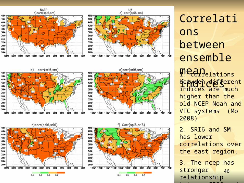
1. correlations between different indices are much higher than the old NCEP Noah and VIC systems (Mo 2008)

2. SRI6 and SM has lower correlations over the east region.

3. The ncep has stronger relationship between SPI6 and SM than the UW

Correlations between ensemble mean indices

4747

IndicesIndices

Correlations among indices are larger than the Correlations among indices are larger than the previous version of models.previous version of models.

The NCEP has stronger correlation between The NCEP has stronger correlation between SPI6 and SM than the UW.SPI6 and SM than the UW.

Correlations between SM and SRI are lower Correlations between SM and SRI are lower over the wet region. (runoff takes water outover the wet region. (runoff takes water out

from the soil?)from the soil?)