CS 177 - Fall 2010

Homework 3: Vector Field DecompositionDue November 18th before midnight

Please send your pdf and code to fferrari@caltech.edu

1 Differential Forms1.1 Vectors and CovectorsYou’re probably very familiar with vectors in the plane. For reasons that will become clear later, it is also usefulto understand the notion of covectors. Consider the following question:

What are all the linear functions that map a single vector to a scalar?

In other words, what is the form of a linear function f : Rn → R? If you think about it for a while, you realizethat if we have a vector

x =

x1x2...

xn

,the only linear way to produce a scalar is by taking linear combinations of its coordinates:

f (x) =

n∑i=1

αixi,

(where α1, α2, . . . , αn ∈ R are constants). In other words, any such function f is completely defined by asequence of n real numbers. Sounds a lot like a vector, doesn’t it?

In fact, a linear function on a single vector is what we call a covector. Alternatively, we sometimes refer tovectors and covectors as tangents and cotangents, respectively. Superficially, a covector looks a lot like a vector.After all, it can be specified using precisely the same amount of information. What distinguishes a covectorfrom a vector, however, is that it acts on a vector to produce a scalar. For this reason, it’s often convenientto think of vectors and covectors as being represented by columns and rows of matrices, respectively. Forexample, we might represent a covector α as

α =[α1 α2 · · · αn

].

Pairing α with our vector x then becomes

α(x) =[α1 α2 · · · αn

] x1x2...

xn

.At this point you might say that this pairing looks a lot like the typical dot product of two vectors, and

indeed it does! However, this similarity is merely a consequence of working in the plane. When we startworking with curved surfaces (such as the sphere), we will find that the inner product no longer looks like asimple pairing and will have to be careful to distinguish between the two.

1.2 Tensors and Differential FormsRecall our definition of a covector as “a function that takes linear combinations of the coordinates of theinput to produce a scalar.” A tensor is similar to a covector, except that it operates on multiple vectors andcovectors, and takes linear combinations of products of their coordinates. For instance, suppose we have avector x = [x1 x2] and a covector α = [α1 α2]T . A tensor t might operate on both x and α to produce a scalar inthe following way:

1

t(x, α) = 3x1α1 − x1α2 + 4x2α2.

In this case, we can also express t using matrix notation:

t(x, α) =[α1 α2

] [ 3 0−1 4

] [x1x2

].

In general, however, a tensor may map many vectors and covectors to a scalar – not just one of each – so wecannot always express it as a matrix operation. If a tensor maps k vectors and l covectors to a scalar, we call ita “k-times covariant, l-times contravariant” tensor.

Finally, a differential form or differential k-form is a k-times covariant antisymmetric tensor. In otherwords, it’s an object that eats k vectors and spits out a scalar (in a linear way!), and whose sign changes if weswap any pair of arguments. For instance, if α is a 3-form and u, v, and w are vectors, then

α(u, v,w) = −α(w, v, u),

etc. Note that a differential 1-form is the same thing as a covector! Differential forms play an importantrole in geometry and physics, and are often used to represent physical quantities as we’ll see in some of ourapplications. Finally, it is important to note that while most authors make a linguistic distinction between a“vector” and a “vector field,” many do not make the distinction between a “differential form” and a “differentialform field” – the former is simply used interchangeably.

2 Exterior CalculusYou’re probably familiar with vector calculus which consists of operations on “primal” objects such as vectorfields. It is also possible to define an exterior calculus that consists of operations on “dual” objects suchas covectors and differential forms. The duality between the two makes it possible to define any differentialoperator from vector calculus using the language of exterior calculus. One reason why this approach is nicefrom a practical point of view is that exterior calculus has only a single differential operator, called the exteriorderivative, which is denoted d. In the discrete setting, this means that only one differential operator ever hasto be defined and implemented. Here are a few typical differential operators from vector calculus expressedusing the exterior derivative1

∇ f = d f∇ × F = ?dF∇ · F = ?d ? F

The additional map ? is called the Hodge star and introduces another kind of duality within exterior calcu-lus – we will discuss the Hodge star in more detail later. It is also important to note that covector fields are aspecial case of something called a differential form. In particular, covector fields are referred to as 1-forms and“look” much like vector fields. Another common special case is the 0-form, which can be thought of as a scalarfield. You will often see differential forms written in coordinate notation where the magnitude is given for eachprincipal direction. For example, a 1-form α = dx − ydz basically looks like a vector field whose magnitude is1 in the x-direction, 0 in the y-direction, and −y in the z-direction. Much like the gradient operator maps ascalar field to a vector field, the exterior derivative will map a 0-form to a 1-form. More generally, the exteriorderivative maps a k-form to a (k + 1)-form. Finally, the exterior derivative has the important property thatd d = 0.

2.1 Discrete Exterior CalculusIn order to actually compute with exterior calculus, we need to define a discrete exterior calculus (DEC) thatoperates on quantities defined over some discrete differential geometry. In particular, we will define discretedifferential forms as quantities stored on simplicial meshes2, and discrete differential operators that act onthese forms in a way that faithfully mirrors the behavior of the smooth operators.

1Technically speaking these operators are not identical since the operators from vector calculus operate on the tangent bundle whereasthe operators from exterior calculus operate on the cotangent bundle. Since these two spaces are dual, however, there exists a pair of verysimple operators ] (sharp) and [ (flat) which can be used to convert an object from vector calculus to exterior calculus and then back again.For instance, we should really write ∇ × F =

[?

(dF[

)]]if we want the two operations to be truly identical maps.

2Most operations in DEC are well-defined for more general cell complexes, but we will stick to simplicial complexes for simplicity.

2

2.2 Discrete Differential FormsDiscrete differential forms actually have a very simple representation: a k-form is represented by a singlescalar quantity at each k-dimensional simplex of the mesh. So for instance, a 0-form stores a scalar value ateach vertex, a 1-form stores a scalar value at each edge, etc. For 0-forms, you should think of this scalar assimply a point sample of a scalar-valued function. For 1-forms, you should think of this scalar as the totalcirculation along that edge. In other words, if you think of a smooth covector field as passing over an edge,then the scalar will tell you how much total “stuff” is moving parallel to that edge. In general, you can thinkof a discrete k-form as the integral of the evaluation of a smooth k-form over each k-simplex.

In addition to knowing how much stuff is moving through each simplex, we also need to know in whichdirection the stuff is moving. In other words, if we have an edge between vertices a and b, we need to knowwhether the stuff is flowing from a to b or from b to a. Hence, we give each edge an orientation (either a tob or b to a) that gives us a canonical direction along which stuff flows. Then a positive scalar on this edgeindicates that stuff is flowing in the canonical direction, and a negative scalar indicates that stuff is flowing inthe opposite direction. It doesn’t matter how we pick this orientation as long as we are consistent.

2.2.1 Discretizing Smooth Forms

Quite often, integration of a smooth form over a simplex is done via numerical quadrature. Numerical quadra-ture picks a collection of quadrature points xi and corresponding quadrature weights wi, and approximates anintegral using a weighted sum of function values at the quadrature points. For example, the integral of afunction f over a domain Ω would be approximated as∫

Ω

f (x)dx ≈ V(Ω)∑

i

wi f (xi)

where V(Ω) is the volume of Ω.For functions defined over simplices, there are a number of possible choices for weights and quadrature

points – the choice of which quadrature to use depends on the desired accuracy and the degree of the functionbeing integrated. For instance, one-point Gaussian quadrature on a simplex places a single quadrature pointof weight one at the barycenter of the simplex; for a linear function f , this choice of quadrature will in fact givethe exact answer.

Exercise 1. Given the oriented simplicial complex depicted below and the smooth 1-form ω = 2xdy − ydx,compute the corresponding discrete 1-form (i.e., give the value stored on each edge).

(0,0) (1,0)

(1,1)(0,1)

e1

e2

e3

e5

e4

Coding 1. Starting with the template below, write a MATLAB routine that discretizes the smooth 1-form

ω(x, y) = 2e−(x2+y2) ((x + y)dx + (y − x)dy) .

Approximate the integral over each edge with a single quadrature point located at the edge midpoint.You can test whether your routine is working properly by temporarily replacing ω with the linear 1-formω = 2xdy − ydx and running it on the mesh file test.obj, which corresponds to the discretization perfomed inthe previous exercise.

3

function omega = discretize_oneform( V, E )% function omega = discretize_oneform( V, E )%% INPUT:% V - dense 2x|V| matrix of vertex positions% E - dense |E|x2 matrix of edges as 1-based indices into vertex list%% OUTPUT:% omega - |E|x1 vector of discrete 1-form values stored on edges%

2.2.2 Interpolating Discrete Forms

v

1

0

0

Although we can generally perform all of our computations directly using discrete differential forms, it issometimes necessary to construct a smooth form corresponding to a discrete form. One way to construct sucha form is via interpolation. The Whitney forms or Whitney bases provide a set of smooth forms that interpolatediscrete forms defined on a simplicial complex.

The Whitney 0-forms are basis elements for forms defined on vertices, and are denoted φi where i is thevertex of interest. In fact, φi is simply the hat function on vertex i, i.e., the unique function that equals one atvertex i, zero at all other vertices, and is affine over each 2-simplex (see illustration above, left).

Whitney 1-forms interpolate values stored on edges, and are denoted φi j where the edge of interest is ori-ented away from vertex i and toward vertex j. The 1-form bases can be expressed in terms of the 0-formbases:

φi j = φidφ j − φ jdφi

where d is the (smooth) exterior derivative on 0-forms – see the next section for details. Notice that theorientation of the edge (i to j vs. j to i) does matter here since φi j is antisymmetric with respect to i and j,i.e., φi j = −φ ji. An illustration of a discrete 1-form on a triangle interpolated using the Whitney 1-form basis isshown above (right). Edge labels indicate the value of the discrete form on each edge and arrows indicate thedirection and magnitude of the interpolated field.

The Whitney 2-forms interpolate values stored on faces, and are denoted φi jk where the face of interestcontains vertices i, j, and k. The 2-form bases are simply piecewise constant functions that equal 1/A insidethe face (i, j, k) and zero elsewhere, where A is the area of the face.

(Note: you may wish to read the section on the exterior derivative before continuing with the followingexercises.)

4

Exercise 2. The barycentric coordinates for a point p in a simplex σ give, roughly speaking, the proximity ofp to each of the vertices of σ. More specifically, the ith barycentric coordinate function λi : |σ| → R is the uniqueaffine function that equals one at vertex i and zero at all other vertices. In other words, λi(v j) = δi j (where δ isthe Kronecker delta). Make a (simple!) argument that on a 2-simplex, λi(p) is the same as the ratio

f (p) =〈p, j, k〉〈i, j, k〉

where j and k are the indices of the other two vertices in the 2-simplex and 〈i, j, k〉 denotes the area of thetriangle with vertices vi, v j, and vk.

vi

p

vj vk

(Hint: think about the gradient of the area of a triangle. In the remaining exercises, you may find it conve-nient to denote the rotation in the plane of a vector v by an angle π/2 by v⊥.)

Exercise 3. Derive an expression for Whitney 1-form bases on a simplicial 2-complex that is suitable forimplementation. In particular, for a 2-simplex σ with vertices vi, v j, and vk, give an expression for φi j(p) purelyin terms of triangle areas and edge vectors, where p is any point inside the simplex.

(Hint: the Whitney 0-form bases restricted to a single simplex are merely the barycentric coordinate functionsfor that simplex.)

Exercise 4.Let e1, e2, and e3 be the three edge vectors of a triangle oriented as in the figure below. Show that

e⊥2 + e⊥3 = −e⊥1 .

(This fact will be useful in the next exercise.)

e1

e2

e3e1

e2

e3

Exercise 5. One nice property of Whitney forms is that interpolating with Whitney forms and then applyingthe (smooth) exterior derivative is the same as applying the (discrete) exterior derivative and then interpolat-ing with Whitney forms. In other words, the following diagram commutes:

5

ωk dk−−−−−−→ ωk+1

φk

y yφk+1

ωk dk−−−−−−→ ωk+1

where ωk is a discrete k-form and ωk is a smooth k-form. Consider a simplicial 2-complex K and prove thatthis relationship holds in the case of k = 0, i.e., show that

φ1d0ω = d0φ0ω

for any discrete 0-form ω on K.

(Hint: consider a single 2-simplex; the results of the previous three exercises will be useful.)

Coding 2. Write a MATLAB routine that interpolates a discrete 1-form over a single 2-simplex in the planeusing the Whitney 1-form bases, starting with the template below. (In other words, implement the expressionderived in Exercise 3.) This routine will be used to display the vector field decomposition produced in a laterexercise. You may find it useful to use the subroutine A = triangle area( a, b, c ). Additionally, youshould test your routine by running the script draw whitney oneform.m. This script produces an output fileoneform.ps which displays the Whitney 1-form basis for a single edge in a triangle and should match theappearance of the illustration above. Please include a printout of this output with your written assignment.

function u = oneform( V, omega, p )% function u = oneform( V, omega, p )%% Interpolates a discrete 1-form using the Whitney basis.%% INPUT:% V - 2x3 matrix; columns give vertex coordinates of vertices in triangle a,b,c% omega - 3x1 vector of 1-form values stored on edges (a,b), (b,c), (c,a), resp.% p - 2x1 vector representing sample location%% OUTPUT:% u - 2x1 vector giving interpolated 1-form at p%

2.3 Discrete Exterior DerivativeRecall that the smooth exterior derivative d maps a k-form to a (k + 1)-form. In our discrete framework, thismeans we want an operator that maps a scalar quantity stored on k-dimensional simplices to a scalar quantityon (k + 1)-dimensional simplices. The discrete version of the exterior derivative turns out to be a very simpleprocedure: to get the scalar value for a particular (k + 1)-simplex, we basically just add up the values stored onall the k-simplices along its boundary! With one caveat: we need to be careful about orientation. Since the signof the scalar value changes depending on the orientation of each simplex (and since this choice is arbitrary),we need to take orientation into account in our sum. In general this means that if the orientation of a simplexand one of the simplices on its boundary are opposite, we subtract the value stored on the boundary simplexfrom our sum; otherwise, we add this value.

For instance, in the special case of a 0-form (i.e., a scalar function on vertices), the exterior derivative isincredibly simple to compute: to get the scalar value for an edge whose orientation is from a to b, simplysubtract the value at a from the value at b!

Exercise 6. Let α be the discrete 1-form on the mesh pictured below given by the following table:

e1 2e2 -1e3 3e4 -4e5 7

6

Compute the discrete 2-form dα, paying careful attention to orientation.

Exercise 7. The discrete exterior derivative on k-forms can be represented by a matrix dk ∈ Rm×n where n is

the number of k-simplices in the complex, m is the number of (k + 1)-simplices. Entry (i, j) of dk equals ±1 if theith (k + 1)-simplex contains the jth k-simplex, where the sign is positive if the orientations of the two simplicesagree and negative otherwise. (All other entries in the matrix are zero.) Compute the matrix representationsfor d0 and d1 on the mesh pictured below, and verify that d1d0 = 0.

v1 v2

v3v4

e1

e2

e3

e5

e4

f1

f2

Coding 3. Write a MATLAB routine that builds (sparse!) matrices representing the discrete exterior deriva-tives on 0- and 1-forms, starting with the template below. Edges should be oriented such that each edge pointsfrom the smaller to the larger index. Faces should be oriented according to the input. The input to this routineis slightly different than in the previous assignment: rather than a pair (V, F) where each row of F is a listof vertex indices for a face, the routine accepts a triple (V, E, F) where each row of E gives a pair of vertexindices defining an edge and each row of F gives a triple of edge indices defining a face. Additionally, the signof edge indices indicates whether they agree (positive) or disagree (negative) with the orientation of that face.The routine [V,E,F] = read mesh( filename ) (provided) produces data in this format from a WavefrontOBJ mesh. You can test your code by running it on the mesh test.obj – this mesh corresponds to the oneused in the previous exercise3 You should also test that repeated application of the exterior derivative equalszero, i.e., that d1*d0 yields a matrix of all zeros in MATLAB.

function [d0,d1] = build_exterior_derivatives( V, E, F )% function [d0,d1] = build_exterior_derivatives( V, E, F )%% INPUT:% V - dense 2x|V| matrix of vertex positions% E - dense |E|x2 matrix of edges as 1-based indices into vertex list% F - dense |F|x3 matrix of faces as 1-based indices into edge list%% OUTPUT:% d0 - sparse |E|x|V| matrix representing discrete exterior derivative on 0-simplices% d1 - sparse |F|x|E| matrix representing discrete exterior derivative on 1-simplices%

2.3.1 Mesh Traversal

Because the matrices d0 and d1 contain indicence information, they can also be used to traverse the mesh. InMATLAB, these matrices can be used in conjunction with the commands find and unique to iterate overmesh elements in a number of ways. For instance, suppose we wish to visit each face in the mesh and grab theindices of its three vertices. We might write something like this:

3Be warned, however, that depending on how you write your code, edge indices might not match those in the figure! Hence d0 and d1might have rows and columns (respectively) swapped relative to your answer for the previous exercise.

7

nFaces = size( d1, 1 );

for i = 1:nFaces

% initialize an empty list of vertex indicesind = [];

for j = find( d1( i, : )) % iterate over this face’s edgesfor k = find( d0( j, : )) % iterate over this edge’s vertices

% append the current vertex index to the listind = [ ind, k ];

endend

% eliminate redundant vertex indices from the listI = unique( I );

end

The find command returns a list of the indices of all non-zero entries in a given vector. So for instance,since the ith row of d1 corresponds to the ith face in the mesh, we can run find on this row to get the indicesof all the incident edges. The unique command removes any element of a list that appears more than once.In our example above every vertex is found in two edges of a given face, so we remove redundant indices withunique. This type of mesh traversal will be useful in later coding exercises.

2.3.2 Smooth Exterior Derivative on 0-forms

For some of the above exercises it will be necessary to compute the exterior derivative of smooth 0-forms incoordinates. Such a computation is actually quite simple: for instance, given a (smooth) 0-form f : R2 → R, itsexterior derivative is given by

d f =∂ f∂x

dx +∂ f∂y

dy.

The forms dx and dy can be thought of as standard bases for the (dual) plane. It is therefore sometimes

convenient to think of d f as being merely the transpose of the column vector ∇ f =

[∂ f /∂x∂ f /∂y

]. Also note that d

is a linear operator since ∂∂x and ∂

∂y are both linear operators.

Exercise 8. Compute (in coordinates) the smooth exterior derivative of the 0-form α : R3 → R given by

α = y cos z + 4 sin x.

8

2.4 Hodge Star2.4.1 Circumcentric Dual

primal

dual

In addition to the typical mesh used to discretize our geometry, many operations in DEC require that wedefine a dual mesh or dual complex. In general, the dual of an n-dimensional simplicial complex identifiesevery k-simplex in the primal (i.e., original) complex with a unique (n − k)-cell in the dual complex. In a two-dimensional simplicial complex, for instance, primal vertices are identified with dual faces, primal edges areidentified with dual edges, and primal faces are identified with dual vertices. Note that the dual cells are notalways simplices! However, they can be described as a collection of simplices. (See illustrations above.)

The combinatorial relationship between the two meshes is often not sufficient, however. We may also needto know where the vertices of our dual mesh are located. In the case of a simplicial n-complex embedded in Rn,dual vertices are often placed at the circumcenter of the corresponding primal simplex. The circumcenter of ak-simplex is the center of the unique (k − 1)-sphere containing all of its vertices; equivalently, it is the uniquepoint equidistant from all vertices of the simplex (this latter definition is perhaps more useful in the case of a0-simplex). This particular dual is known as the circumcentric dual. The following exercises prove a statementwhich can be useful when constructing the circumcentric dual of a given mesh.

Exercise 9. Show that the circumcenter of a triangle is the intersection of the perpendicular bisectors of itsedges.

(Hint: use the symmetry of isosceles triangles.)

Exercise 10. Consider the lines passing through the circumcenters of the faces of a tetrahedron, each oneperpendicular to its associated face. Show that the circumcenter of the tetrahedron is the intersection of these

9

four lines. Generalize your proof to show that the circumcenter of a k-simplex is the intersection of the k + 1orthogonal lines through the circumcenters of its faces.

Coding 4. Write a MATLAB routine that computes the circumcenters of all 0-, 1-, and 2-simplices in a givensimplicial 2-complex, starting with the template below. Note that the complex is embedded in R2, hence eachcolumn of V gives the coordinate of a vertex. Once you have computed the circumcenters, call the routinewrite circumcentric subdivision( filename, d0, d1, c0, c1, c2 ) to verify your results. Thisroutine will produce a PostScript drawing of the circumcentric subdivision of the original simplicial complex –please turn a printout of this file in with your written exercises.

function [c0,c1,c2] = compute_circumcenters( V, d0, d1 )% function [c0,c1,c2] = compute_circumcenters( V, d0, d1 )%% INPUT:% V - dense 2x|V| matrix of vertex positions% d0 - sparse |E|x|V| matrix representing discrete exterior derivative on 0-simplices% d1 - sparse |F|x|E| matrix representing discrete exterior derivative on 1-simplices%% OUTPUT:% c0 - dense 2x|V| matrix of vertex circumcenters% c1 - dense 2x|E| matrix of edge circumcenters% c2 - dense 2x|F| matrix of face circumcenters

2.4.2 Discrete Hodge Star

primal 1-form (circulation) dual 1-form (flux)

In (smooth) exterior calculus, the Hodge star identifies a k-form with a particular (n k)-form (called itsHodge dual), and represents a duality somewhat like the duality between vectors and 1-forms. We can of

10

course define an analogous duality in discrete exterior calculus: the discrete Hodge dual of a (discrete) k-formon the primal mesh is an (n − k)-form on the dual mesh. Similarly, the Hodge dual of an k-form on the dualmesh is a k-form on the primal mesh. Discrete forms on the primal mesh are called primal forms and discreteforms on the dual mesh are called dual forms. Given a discrete form α (whether primal or dual), its Hodgestar is typically written as ?α. The star is sometimes used to denote a dual cell as well. For instance, if σ is asimplex in a primal complex, ?σ is the corresponding cell in the dual complex.

Unlike smooth forms, discrete primal and dual forms live in different spaces (so for instance, discrete primalk-forms and dual k-forms cannot be added to each other). In fact, primal and dual forms often have different(but related) physical interpretations. For instance, a primal 1-form might represent the total circulation alongedges of the primal mesh, whereas in the same context a dual 1-form might represent the total flux throughthe corresponding dual edges (see illustration above). Of course, these two quantities are related, and it leadsone to ask, “precisely how should the Hodge star be defined?”

It turns out that there are several ways to define the discrete Hodge star, but most common is the diagonalHodge star, which we will use throughout the rest of this assignment. Consider a primal k-form α defined ona complex K and let K′ be the corresponding dual complex. If αi is the value of α on the k-simplex σi, then thediagonal Hodge star is defined by

?αi =| ? σi|

|σi|αi

for all i, where |σ| indicates the volume of σ (note that if σ is a 0-cell then |σ| = 1) and ?σ ∈ K′. Inother words, to compute the dual form we simply multiply the scalar value stored on each cell by the ratio ofcorresponding dual and primal volumes.

If we remember that a discrete form can be thought of as a smooth form integrated over each cell, thisdefinition for the Hodge star makes perfect sense: the primal and dual quantities should have the samedensity, but we need to account for the fact that they are integrated over cells of different volume. We thereforenormalize by a ratio of volumes when mapping between primal and dual. This particular Hodge star is calleddiagonal since the ith element of the dual form depends only on the ith element of the primal form. Hencethe Hodge star can be implemented as multiplication by a diagonal matrix whose entries are simply the ratiosdescribed above. Clearly, then, the Hodge star that takes dual forms to primal forms (the dual Hodge star) isthe inverse of the one that takes primal to dual forms (the primal Hodge star).

Coding 5. Write a MATLAB routine that builds (sparse!) diagonal matrices representing the diagonal Hodgestar operators on 0- 1- and 2-forms, starting with the template below. You may find it useful to use thesubroutine A = triangle area( a, b, c ).

function [star0,star1,star2] = build_hodge_stars( d0, d1, c0, c1, c2 )% function [star0,star1,star2] = build_hodge_stars( d0, d1, c0, c1, c2 )%% INPUT:% d0 - sparse |E|x|V| matrix representing discrete exterior derivative on 0-simplices% d1 - sparse |F|x|E| matrix representing discrete exterior derivative on 1-simplices% c0 - dense 2x|V| matrix of vertex circumcenters% c1 - dense 2x|E| matrix of edge circumcenters% c2 - dense 2x|F| matrix of face circumcenters%% OUTPUT:% star0 - sparse diagonal |V|x|V| matrix representing Hodge star on primal 0-forms% star1 - sparse diagonal |E|x|E| matrix representing Hodge star on primal 1-forms% star2 - sparse diagonal |F|x|F| matrix representing Hodge star on primal 2-forms%

11

3 Hodge Decomposition3.1 Decomposition of Vector Fields

= +

curl-freevector field divergence-free

+

(harmonic=0)

The Hodge decomposition theorem states that any vector field X : R3 → R3 with compact support can bewritten as a unique sum of a divergence-free component ∇ f , a curl-free component ∇ × A, and a harmonic partH:

X = ∇ f + ∇ × A + H. (1)

Here f is called a scalar potential and A is called a vector potential. H is a harmonic vector field, i.e., avector field such that both ∇ · H = 0 and ∇ × H = 0. Intuitively, ∇ f accounts for sources and sinks in X, ∇ × Aaccounts for vortices, and H accounts for any constant motion. The Hodge decomposition theorem also appliesto two-dimensional vector fields X : R2 → R2, but in this case A is a scalar field which can be thought of as thesigned magnitude of a vector potential sticking out of the plane. The image above gives an example of Hodgedecomposition for a vector field with a zero harmonic component.

Using a little bit of knowledge about vector calculus, we can come up with a simple procedure for actuallyfinding the Hodge decomposition of a vector field. First, recall that ∇ × ∇ f = 0 and that ∇ · ∇ × A = 0. Inother words, the curl of a curl-free field is zero, and the divergence of a divergence-free field is also zero! Alsoremember that both the curl and the divergence of a harmonic vector field are identically zero. Then takingthe divergence of equation (1) gives us

∇ · X = ∇ · ∇ f + ∇ · ∇ × A + ∇ · H= ∇2 f + 0 + 0= ∇2 f

(2)

where ∇2 = ∇ · ∇ is the Laplacian operator. Similarly, taking the curl of equation 1 gives us

∇ × X = ∇ × ∇ f + ∇ × ∇ × A + ∇ × H= 0 + ∇ × ∇ × A + 0= ∇ × ∇ × A.

(3)

We can solve equations (2) and (3) for the potentials f and A, and then use these two quantities to computethe harmonic part

H = X − ∇ f − ∇ × A. (4)

3.2 Decomposition of FormsOf course, since vector calculus and exterior calculus are dual, we can translate this procedure into the lan-guage of exterior calculus. By doing so, we will be able to easily compute the Hodge decomposition of a vectorfield using our existing DEC framework.

Exercise 11. Using the identities from section 2, rewrite the Hodge decomposition theorem in the languageof exterior calculus, where ω is any 1-form, α is a 0-form representing the scalar potential, β is a 2-formrepresenting the vector potential, and γ is a harmonic form. Similar to a harmonic vector field, a harmonic

12

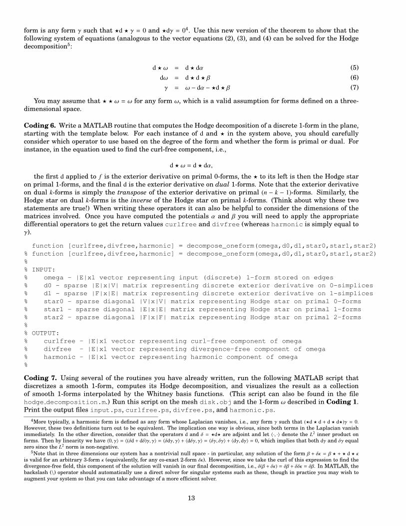
form is any form γ such that ?d ? γ = 0 and ?dγ = 04. Use this new version of the theorem to show that thefollowing system of equations (analogous to the vector equations (2), (3), and (4) can be solved for the Hodgedecomposition5:

d ? ω = d ? dα (5)dω = d ? d ? β (6)γ = ω − dα − ?d ? β (7)

You may assume that ? ? ω = ω for any form ω, which is a valid assumption for forms defined on a three-dimensional space.

Coding 6. Write a MATLAB routine that computes the Hodge decomposition of a discrete 1-form in the plane,starting with the template below. For each instance of d and ? in the system above, you should carefullyconsider which operator to use based on the degree of the form and whether the form is primal or dual. Forinstance, in the equation used to find the curl-free component, i.e.,

d ? ω = d ? dα,

the first d applied to f is the exterior derivative on primal 0-forms, the ? to its left is then the Hodge staron primal 1-forms, and the final d is the exterior derivative on dual 1-forms. Note that the exterior derivativeon dual k-forms is simply the transpose of the exterior derivative on primal (n − k − 1)-forms. Similarly, theHodge star on dual k-forms is the inverse of the Hodge star on primal k-forms. (Think about why these twostatements are true!) When writing these operators it can also be helpful to consider the dimensions of thematrices involved. Once you have computed the potentials α and β you will need to apply the appropriatedifferential operators to get the return values curlfree and divfree (whereas harmonic is simply equal toγ).

function [curlfree,divfree,harmonic] = decompose_oneform(omega,d0,d1,star0,star1,star2)% function [curlfree,divfree,harmonic] = decompose_oneform(omega,d0,d1,star0,star1,star2)%% INPUT:% omega - |E|x1 vector representing input (discrete) 1-form stored on edges% d0 - sparse |E|x|V| matrix representing discrete exterior derivative on 0-simplices% d1 - sparse |F|x|E| matrix representing discrete exterior derivative on 1-simplices% star0 - sparse diagonal |V|x|V| matrix representing Hodge star on primal 0-forms% star1 - sparse diagonal |E|x|E| matrix representing Hodge star on primal 1-forms% star2 - sparse diagonal |F|x|F| matrix representing Hodge star on primal 2-forms%% OUTPUT:% curlfree - |E|x1 vector representing curl-free component of omega% divfree - |E|x1 vector representing divergence-free component of omega% harmonic - |E|x1 vector representing harmonic component of omega%

Coding 7. Using several of the routines you have already written, run the following MATLAB script thatdiscretizes a smooth 1-form, computes its Hodge decomposition, and visualizes the result as a collectionof smooth 1-forms interpolated by the Whitney basis functions. (This script can also be found in the filehodge decomposition.m.) Run this script on the mesh disk.obj and the 1-form ω described in Coding 1.Print the output files input.ps, curlfree.ps, divfree.ps, and harmonic.ps.

4More typically, a harmonic form is defined as any form whose Laplacian vanishes, i.e., any form γ such that (?d ? d + d ? d?)γ = 0.However, these two definitions turn out to be equivalent. The implication one way is obvious, since both terms in the Laplacian vanishimmediately. In the other direction, consider that the operators d and δ = ?d? are adjoint and let 〈·, ·〉 denote the L2 inner product onforms. Then by linearity we have 〈0, γ〉 = 〈(δd + dδ)γ, γ〉 = 〈δdγ, γ〉 + 〈dδγ, γ〉 = 〈δγ, δγ〉 + 〈dγ, dγ〉 = 0, which implies that both dγ and δγ equalzero since the L2 norm is non-negative.

5Note that in three dimensions our system has a nontrivial null space - in particular, any solution of the form β + δκ = β ? + ? d ? κis valid for an arbitrary 3-form κ (equivalently, for any co-exact 2-form δκ). However, since we take the curl of this expression to find thedivergence-free field, this component of the solution will vanish in our final decomposition, i.e., δ(β + δκ) = δβ + δδκ = δβ. In MATLAB, thebackslash (\) operator should automatically use a direct solver for singular systems such as these, though in practice you may wish toaugment your system so that you can take advantage of a more efficient solver.

13

Recall that the 1-form ω used in discretize oneform is given by

ω(x, y) = 2e−(x2+y2) ((x + y)dx + (y − x)dy) ,

which is depicted at the beginning of this section6. The Hodge decomposition of ω can be expressed analyt-ically as

ω(x, y) = ∇g(x, y) + ∇ × g(x, y)

where g = α = β serves as both the scalar and the vector potential, and is given by

g(x, y) = −ex2+y2.

Hence, the potentials α and β should both look like a Gaussian “bump,” and the curl-free and divergence-free components ∇α and ∇ × β of ω should look like the source and vortex pictured at the beginning of thissection.

When debugging, you may find it useful to discretize ∇α and ∇ × β directly and compare with the 1-formscomputed via Hodge decomposition. (At the very least, you should verify that your output files roughly matchthe appearance of the images above.) Additionally, three alternative definitions for omega are provided to helpverify the correctness of your routines: a purely curl-free omega, a purely divergence-free omega, and a purelyharmonic omega. For each of these cases Hodge decomposition should reproduce the input exactly in one ofthe three components (curlfree, divfree, or harmonic) while the other two components should vanish.(Simply uncomment the appropriate line to use one of these test cases.) Additionally, two meshes are providedfor testing: disk.obj and annulus.obj. The harmonic part of the output should always be zero for the disk,and you should find a non-zero harmonic part for 1-forms over the annulus.

stderr = 2;input_filename = ’../meshes/disk.obj’;

fprintf( stderr, ’Reading...\n’ );[V,E,F] = read_mesh( input_filename );

fprintf( stderr, ’Building exterior derivatives...\n’ );[d0,d1] = build_exterior_derivatives( V, E, F );

fprintf( stderr, ’Computing circumcenters...\n’ );[c0,c1,c2] = compute_circumcenters( V, d0, d1 );

fprintf( stderr, ’Writing circumcentric subdivision...\n’ );write_circumcentric_subdivision( ’subdivision.ps’, d0, d1, c0, c1, c2 );

fprintf( stderr, ’Building Hodge stars...\n’ );[star0,star1,star2] = build_hodge_stars( d0, d1, c0, c1, c2 );

fprintf( stderr, ’Discretizing smooth 1-form...\n’ );omega = discretize_oneform( V, E );% Some test cases:% omega = d0*rand(size(V,2),1); % curl-free test case% omega = (star1ˆ-1)*d1’*star2*rand(size(F,1),1); % divergence-free test case% omega = null( d0*(star0ˆ-1)*d0’*star1 + (star1ˆ-1)*d1’*star2*d1 ); % harmonic test case

fprintf( stderr, ’Decomposing discrete 1-form...\n’ );[ curlfree, divfree, harmonic ] = decompose_oneform( omega, d0, d1, star0, star1, star2 );

M = max( abs( omega ));

6Note that this 1-form does not have compact support, which was one of the requirements of the Hodge decomposition theorem!Numerically, however, the field decays fast enough that we can treat it as compact – in general certain boundary conditions are requiredto deal with non-compactness. For more details, see Tong et al, Discrete Multiscale Vector Field Decomposition, in the Proceedings of ACMSIGGRAPH 2003.

14

fprintf( stderr, ’Interpolating input...\n’ );write_interpolated_vector_field( ’input.ps’, omega/M, d0, d1, c0, c1, c2 );fprintf( stderr, ’Interpolating curl-free component...\n’ );write_interpolated_vector_field( ’curlfree.ps’, curlfree/M, d0, d1, c0, c1, c2 );fprintf( stderr, ’Interpolating divergence-free component...\n’ );write_interpolated_vector_field( ’divfree.ps’, divfree/M, d0, d1, c0, c1, c2 );fprintf( stderr, ’Interpolating harmonic component...\n’ );write_interpolated_vector_field( ’harmonic.ps’, harmonic/M, d0, d1, c0, c1, c2 );

disp( ’Done.’ );

15