1

Clustered Components Analysis for Functional

MRISea Chen, Charles A. Bouman, and Mark J. Lowe

Abstract

A common method of increasing SNR in functional magnetic resonance imaging is to average signaltimecourses across voxels. This technique is potentially problematic because the hemodynamic responsemay vary across the brain. Such averaging may destroy significant features in the temporal evolution of thefMRI response that stem from either differences in vascular coupling to neural tissue or actual differences inthe neural response between two averaged voxels. Two novel techniques are presented in this paper in orderto aid in an improved SNR estimate of the hemodynamic response, while preserving statistically significantvoxel-wise differences. The first technique is signal subspace estimation for periodic stimulus paradigmsthat involves a simple thresholding method. This increases SNR via dimensionality reduction. The secondtechnique that we call clustered components analysis (CCA) is a novel amplitude-independent clusteringmethod based upon an explicit statistical data model. It includes an unsupervised method for estimatingthe number of clusters. Our methods are applied to simulated data for verification and comparison toother techniques. A human experiment was also designed to stimulate different functional cortices. Ourmethods separated hemodynamic response signals into clusters that tended to be classified according totissue characteristics.

Keywords

functional MRI, BOLD signal estimation, clustering methods, EM algorithm, hemodynamic response,functional neuroimaging, brain activation, vascular coupling, independent components analysis.

S. Chen and M. J. Lowe are with the Division of Imaging Sciences, Department of Radiology, Indiana UniversitySchool of Medicine, Indianapolis, Indiana, and the Department of Biomedical Engineering, Purdue University, WestLafayette, Indiana. E-mail: sechen@iupui.edu, mjlowe@iupui.edu .

C. A. Bouman is with the School of Electrical and Computer Engineering, Purdue University, West Lafayette,Indiana. E-mail: bouman@ecn.purdue.edu.

This research was supported in part by an NSF-IGERT PTDD training grant DGE-99-72770.To appear in the IEEE Transactions on Medical Imaging.

2

I. Introduction

Functional magnetic resonance imaging (fMRI) has emerged as a useful tool in the study of brain

function. This imaging modality utilizes the fact that the MRI signal is sensitive to many of the

hemodynamic parameters that change during neuronal activation (e.g. blood flow, blood volume,

oxygenation). The changes in these parameters cause small intensity differences between properly

weighted MR images acquired before and during neuronal activation. Although the contrast can

be produced by a number of different mechanisms, blood oxygenation level dependent (BOLD)

contrast is the method most commonly employed. BOLD contrast is dependent on an decrease in

local deoxy-hemoglobin concentration in an area of neuronal activity [1], [2]. This local decrease

in paramagnetic material increases the apparent transverse relaxation constant T ∗2 , resulting in an

increase of MR signal intensity in the area affected. Other methods of functional MR imaging

contrast include measurement of cerebral blood flow and volume effects [3]. Although fMRI is

widely used, the mechanism of the coupling between brain hemodynamics and neuronal activation

is poorly understood.

Although much of the work in fMRI data analysis has revolved around the creation of statistical

maps and the detection of activation at different voxel locations [4], [5], [6], there also has been

much interest in understanding the BOLD temporal response. Several groups have proposed models

relating the various hemodynamic parameters (blood flow, blood volume, hemoglobin concentration,

etc.) to the BOLD signal [7], [8]. These models all predict a BOLD temporal response to changing

neuronal activity. Verification of the accuracy of these models requires that the predictions be

compared to data. However, the low signal-to-noise ratio (SNR) of fMRI measurements typically

requires averaging of many voxels in order to achieve a statistically significant result. Thus, the

resulting measurement could possibly be a mixture of many different responses. This presents a

possible confound in attempts to develop and validate detailed models of the BOLD response.

Some researchers have attempted to address the issue by using parametric methods [9], [10].

The parametric methods usually assume specific signal shapes (Poisson, Gaussian, Gamma, etc.)

and attempt to extract the associated parameters for which the data best fit. Others have taken

3

a linear systems approach in which the response is modeled as an impulse response convolved

with the stimulus reference function [11], [12]. Exploratory data analysis methods such as principle

components analysis (PCA) [13], [14] and independent components analysis (ICA) [15], [16] are also

commonly used by many groups. Recently, clustering methods [17], [18], [19], [20] have become

popular as well.

In this paper, we address the issue of signal averaging by presenting a novel non-parametric clus-

tering method based upon a statistical data model. Our technique is designed to robustly estimate

the fMRI signal waveforms rather than detect their presence. Specifically, we first select voxels that

contain the fMRI signal using a previously published technique [21]. Then our procedure identi-

fies groups of voxels in fMRI data with the same temporal shape independent of signal amplitude.

Variations in amplitudes may be due to differences in the concentration of hemodynamic events

from partial volume effects or coil geometries. The amplitude variation is explicitly accounted for

in our data model. Each distinct response corresponds to a unique direction in a multidimensional

feature space (see Figure 1).

Fig. 1. Visualization of cylindrical clusters extracted by CCA: Because CCA finds cluster directions inde-pendent of amplitude, the shape of the vector clouds will be cylindrical instead of the more common sphericalclouds around class means extracted by other clustering methods.

Our analysis framework is based upon two distinct steps. In the first step, the dimensionality of

4

the voxel timecourses is reduced and feature vectors are obtained. The noise in the feature vectors

is then whitened in preparation for the next step. The second step consists of our novel clustering

technique that we call clustered components analysis (CCA).

The dimensionality reduction used in this paper is similar to the method described by Bullmore, et

al. [22]. Their method decomposes the temporal response at each voxel into harmonic components

corresponding to a sine and cosine series expansion at the appropriate period. We have developed

a method to further decrease dimensionality by estimating an M dimensional signal subspace

[23]. Although signal subspace estimation (SSE) is not new [24], [25], our method uses a simple

thresholding technique and is quite effective. It is implemented by estimating the signal covariance

as the positive definite part of the difference between the total signal-plus-noise covariance and the

noise covariance. At this point in our analysis technique, each voxel’s response is represented by

an M dimensional feature vector.

In the second step of our analysis framework, we present a new method for analyzing the multi-

variate fMRI feature vectors that we call clustered components analysis. This method depends on

a explicit data model of the feature vectors and is implemented through maximum likelihood (ML)

estimation via the expectation-maximization (EM) algorithm [26], [27]. An agglomerative cluster

merging technique based on a minimum description length (MDL) criterion [28] is used to estimate

the true number of clusters [29].

Because the truth is not known in a real experiment, synthetic data was generated to test

the performance of our method. Other common methods of multivariate data-driven analysis

techniques (PCA, ICA, and fuzzy clustering) were applied to the same data set and the results

were compared. Finally, a human experiment was performed that stimulated the motor, visual, and

auditory cortices. Our methodology was applied to this data. The goal of the human experiment

was to produce a set of activation data spanning a broad range of cerebral cortex and a diverse set

of neuronal systems. This data set will allow our clustering method to determine the distribution

of distinct temporal responses according either to neuronal system or tissue characteristics.

5

II. Theory

A. Dimensionality Reduction

The first step of our analysis framework is the reduction of dimensionality via decomposition

into harmonic components using least squares fitting. This step is similar to that described in [22].

The next step is a novel method of determining the signal subspace by estimating signal and noise

covariances and performing an eigendecomposition. The final step is a prewhitening of the noise

before application of the clustered components analysis.

A.1 Decomposition into Harmonic Components

In a standard block paradigm, control and active states are cycled in a periodic manner during the

fMRI experiment. Therefore, the response signal should also be periodic. By assuming periodicity,

harmonic components can be used as a basis for decomposition to reduce dimensionality. However,

application of the periodicity constraint is not necessary for the technique described in the next

section.

The data set of an fMRI experiment, D, can be defined as an P × N matrix, where N is the

number of voxels and P is the number of time points. We first remove the baseline and linear drift

components of fMRI data as a preprocessing step [21]. The columns of D are then zero mean, zero

drift versions of the voxel timecourses.

The harmonic components, Al, are a sampling of sines and cosines at the fundamental frequency

of the experimental paradigm, γ (in radians/seconds), and its higher harmonics. The number of

harmonic components, L, is limited by the requirement that there be no temporal aliasing. In other

words, L < ∆tγ2 where ∆t is the temporal sampling period.

Al(t) =

cos(

l+12 γt

)

if l odd

sin(

l2γt)

if l even(1)

for l = [1, 2, · · · , L]

6

We then form a P × L design matrix

A = [a1, · · · , aL] , (2)

where al is a column vector formed by sampling the lth harmonic component at the times corre-

sponding to the voxel samples. Using this notation, the data can then be expressed as a general

linear model [6] where

D = AΘ + ν. (3)

Θ is an L × N harmonic image matrix containing the linear coefficients, and ν is the P × N

dimensional noise matrix.

Assuming all information in the signal is contained within the range A, an estimate Θ can be

computed using a least squares fit, resulting in

Θ = (AtA)−1AtD (4)

where the residual error ε is given by

ε = D −AΘ (5)

= (I −A(AtA)−1At)D (6)

= (I −A(AtA)−1At)ν . (7)

The data set can be expressed in terms of the estimate of the coefficient matrix and the residuals

matrix.

D = AΘ + ε (8)

We denote the estimation error as Θ, where

Θ = Θ−Θ (9)

= (AtA)−1Atν . (10)

A.2 Signal subspace estimation

Our next objective is to identify the subspace of the harmonic components that spans the space

of all response signals. This signal subspace method improves the signal-to-noise ratio by reducing

7

the dimensionality of the data.

The covariance matrices for the signal, signal-plus-noise, and the noise are defined by the following

relations.

Rs =1

NE[

ΘΘt]

Rsn =1

NE[

ΘΘt]

Rn =1

NE[

ΘΘt]

Since we can not observe Θ directly, we must first estimate Rsn and Rn, and then use these matrices

to estimate Rs. With this in mind, we use the following two estimates for Rsn and Rn.

Rsn =1

NΘΘt (11)

Rn = trace{εεt}(AtA)−1/(N(P − L− 2)) , (12)

where ε is computed using (6). The expression for Rn is derived in Appendix I using the assumption

that the noise ν is white and is shown to be an unbiased estimate for Rn. Note that the denominator

of the expression reflects the reduction in degrees of freedom when the 2 nuisance components are

removed. Since Rsn and Rn are both unbiased estimates of the true covariances, we may form an

unbiased estimate of the signal covariance Rs as

Rs = Rsn − Rn . (13)

The corresponding eigendecomposition is then

Rs = UsΛsUst. (14)

Generally, the matrix Rs will have both positive and negative eigenvalues because it is formed by

the subtraction of (13). However, negative eigenvalue in Rs are non-physical since we know that

Rs is a covariance matrix with strictly positive eigenvalues. Therefore we know that the subspace

corresponding to the negative eigenvalues is dominated by noise. We may exploit this fact by

removing the energy in this noise subspace. To do this, we form a new M ×M diagonal matrix Λs,

which contains only the M positive diagonal elements in Λs, and we form a new L ×M modified

8

eigenvector matrix Us consisting of the columns of Us corresponding to the positive eigenvalues in

Λs. The reduced dimension signal component, or eigenimage, can then be written as

Y = U tsΘ. (15)

The eigenimage Y contains the linear coefficients for the eigensequences Σ = AUs.

The clustered components analysis presented in the following section assumes that the noise is

white. Therefore, we apply a whitening filter W to form

Y = WY (16)

as described in Appendix II. The column vectors of Y correspond to M dimensional feature vectors

that describe the timecourse of each voxel. The timecourse realizations of the individual voxels

may be reconstructed via the following relation.

D = ΣW−1Y (17)

B. Clustered Component Analysis

The method of clustered components analysis is developed in this section. The goal of the method

is to cluster voxels into groups that represent similar shapes and to estimate the representative

timecourses. Specifically, we apply the analysis to the feature vectors Y found in (16). The analysis

not only allows for the estimation of cluster timecourses, but also estimates the total number

of clusters automatically. The algorithm consists of two steps. The first step is the estimation

of the timecourses using the expectation-maximization algorithm. Estimation of the number of

clusters occurs in the second step using the minimum description length criterion. The diagram of

Figure 2 illustrates the basic flow of the CCA algorithm, and Figure 3 give a detailed pseudo-code

specification of the CCA algorithm.

B.1 Data model

Let Yn be the nth column of the matrix Y found in (16). Yn is a vector of parameters specifying

the timecourse or the M dimensional feature vector for voxel n. Furthermore, let EK = [e1, · · · , eK ]

9

EvaluateMDL

> 1 Cluster

Yes

NoSelect Number of Clusterswith Minimum MDL Value

Initialize Ko Clusters

For each cluster, compute

1) Priincipal eigenvector

2) Prior probability

M−Step:

For each cluster, compute

1) Expected covariance

2) Expected number of elements

E−Step:

Converged?Yes

No

Merge Most Similar Clusters

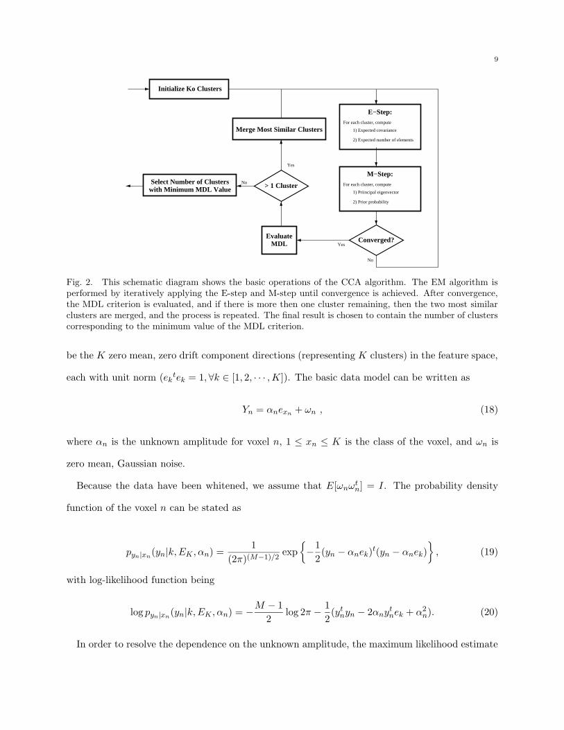
Fig. 2. This schematic diagram shows the basic operations of the CCA algorithm. The EM algorithm isperformed by iteratively applying the E-step and M-step until convergence is achieved. After convergence,the MDL criterion is evaluated, and if there is more then one cluster remaining, then the two most similarclusters are merged, and the process is repeated. The final result is chosen to contain the number of clusterscorresponding to the minimum value of the MDL criterion.

be the K zero mean, zero drift component directions (representing K clusters) in the feature space,

each with unit norm (ektek = 1, ∀k ∈ [1, 2, · · · , K]). The basic data model can be written as

Yn = αnexn + ωn , (18)

where αn is the unknown amplitude for voxel n, 1 ≤ xn ≤ K is the class of the voxel, and ωn is

zero mean, Gaussian noise.

Because the data have been whitened, we assume that E[ωnωtn] = I. The probability density

function of the voxel n can be stated as

pyn|xn(yn|k, EK , αn) =

1

(2π)(M−1)/2exp

{

−1

2(yn − αnek)

t(yn − αnek)

}

, (19)

with log-likelihood function being

log pyn|xn(yn|k, EK , αn) = −

M − 1

2log 2π −

1

2(yt

nyn − 2αnytnek + α2

n). (20)

In order to resolve the dependence on the unknown amplitude, the maximum likelihood estimate

10

αn of the amplitude is found.

αn = argmaxαn

{log pyn|xn(yn|k, EK , αn)}

= yntek (21)

The amplitude estimate in (21) is then substituted into the log-likelihood of (20).

log pyn|xn(yn|k, EK , αn) = −

M − 1

2log 2π −

1

2

(

ytnyn − ek

tynyntek

)

(22)

From (22), the density function may be written as

pyn|xn(yn|k, EK , αn) =

1

(2π)(M−1)/2exp

{

−1

2

(

ytnyn − ek

tynyntek

)

}

. (23)

The class of voxel n is specified by the class label xn, which is an independent, identically

distributed discrete random variable taking on integer values from 1 to K. We define πk = P{Xn =

k} as the prior probabilities that a voxel is of class k. The set of prior probabilities for K classes

are then defined to be ΠK = [π1, · · · , πK ], where∑K

k=1 πk = 1.

Using Bayes rule, the voxel probability density can be written without conditioning on class

label.

pyn(yn|K, EK , ΠK , αn) =K∑

k=1

pyn|xn(yn|k, EK , αn)πk (24)

=K∑

k=1

(

1

(2π)(M−1)/2exp

{

−1

2

(

ytnyn − ek

tynyntek

)

})

πk (25)

We note that this is a Gaussian mixture distribution [30].

The log-likelihood is then calculated for the whole set of voxels.

log py(y|K, EK , ΠK , α) =N∑

n=1

log

(

K∑

k=1

pyn|xn(yn|k, EK , αn)πk

)

=N∑

n=1

log

[

K∑

k=1

(

1

(2π)(M−1)/2exp

{

−1

2

(

ytnyn − ek

tynyntek

)

}

πk

)

]

(26)

B.2 Parameter estimation using the expectation-maximization algorithm

The aim of this section is to estimate the parameters EK and ΠK in the data model. This is

done by finding the maximum likelihood estimates for the log-likelihood given in (26) for a given

11

cluster number K.

(EK , ΠK) = argmaxEK ,ΠK

log py(y|K, EK , ΠK , α) (27)

The maximum likelihood estimates EK and ΠK in (27) are found by using the expectation-

maximization algorithm [26], [30].

In order to compute the expectation step of the EM algorithm, we must first compute the

posterior probability that each voxel label xn is of class k.

pxn|yn(k|yn, K, EK , ΠK , αn) =

pyn|xn(yn|k, EK , αn)πk

∑Kl=1 pyn|xn

(yn|k, EK , αn)πl

(28)

In the expectation step of the EM algorithm, the estimated number of voxels per class N(i)k|K and

the estimated covariance matrix of the class R(i)k|K given the current estimation of the parameters

EK(i) and ΠK

(i) must be computed. See Appendix III-A for more details. Because the EM

algorithm is iterative, the superscripts (i) denote iteration number. The subscript k|K denotes the

parameter corresponding to the kth cluster out of a total of K clusters.

N(i)k|K =

N∑

n=1

pxn|yn(k|yn, EK

(i), ΠK(i), αn) (29)

R(i)k|K =

1

N(i)k|K

N∑

n=1

ynytn pxn|yn

(k|yn, EK(i), ΠK

(i), αn) (30)

In the maximization step of the EM algorithm, the parameters are reestimated from the values

found in the expectation step (see (29) and (30)), yielding EK(i+1) and ΠK

(i+1). Let emax{R} be

the principle eigenvector of R.

e(i+1)k = emax{R

(i)k|K} (31)

π(i+1)k = N

(i)k|K/N (32)

for k ∈ [1, 2, · · · , K] (see Appendix III-B for more details).

(31) and (32) are alternately iterated with (29) and (30) (using (28)). The iterations are stopped

when the difference in the log-likelihood (see (26)) for subsequent iterations is less than an arbitrary

stopping criterion, υ. We then denote the final estimates of the parameters for a given number of

clusters K as EK and ΠK .

12

B.3 Model order identification

Our objective is not only to estimate the component vectors EK and the prior probabilities

ΠK from observations, but also to estimate the number of classes K. We use the minimum de-

scription length (MDL) criterion developed by Rissanen [28], which incorporates a penalty term

KM log(NM)/2. The term NM represents the number of scalar values required to represent the

data, and the term KM represents the number of scalar parameters encoded by EK and ΠK .

MDL(K, EK , ΠK) = − log py(y|K, EK , ΠK , α) +1

2KM log(NM) (33)

The MDL criterion is then minimized with respect to K. This is done by starting with K large, and

then sequentially merging clusters until K = 1. More specifically, for each value of K, the values of

EK , ΠK , and MDL(K, EK , ΠK) are calculated using the EM algorithm from Section II-B.2. Next,

the two most similar clusters are merged, K is decremented to K − 1, and the process is repeated

until K = 1. Finally, we select the value of K (and corresponding parameters EK and ΠK) that

resulted in the smallest value of the MDL criterion.

This merging approach requires that we define a method for selecting similar clusters. For this

purpose, we define the following distance function between the clusters l and m

d(l, m) = σmax(Rl|K) + σmax(Rm|K)− σmax(Rl|K + Rm|K) (34)

where σmax(R) denotes the principal eigenvalue of R. In Appendix IV, we show that this distance

function is an upper bound on the change in the MDL value (see (66)). Therefore, by choosing the

two clusters l and m that minimize the cluster distance,

(l, m) = argminl,m

d(l, m) (35)

we minimize an upper bound on the resulting MDL criterion. The parameters of the new cluster

formed by merging l and m are given by

π(l,m) = πl + πm (36)

e(l,m) = emax{Rl|K + Rm|K} . (37)

13

initialize K to K0

initialize EK0(1) and ΠK0

(1) using (38), (39), and (40)while K > 1

i← 1do

compute the posterior probabilities pxn|yn(k|yn, K, EK , ΠK , αn) for all n using (28)

E-step: compute N(i)k|K and R

(i)k|K using (29) and (30)

M-step: compute E(i+1)K and Π

(i+1)K using (31) and (32)

δ ← log py(y|K, EK(i+1), ΠK

(i+1), α)− log py(y|K, EK(i), ΠK

(i), α)i← i + 1

while δ > υ (where υ is the stopping tolerance)set EK = EK

(i) and ΠK = ΠK(i)

compute MDLK = MDL(K, EK , ΠK) using (33)save EK and ΠK and MDLK

find the two clusters l and m which minimize the distance function d(l, m)using (34) and (35)merge clusters l and m to form EK−1

(1) and ΠK−1(1) using (36) and (37)

K ← K − 1endchoose K and the corresponding EK and ΠK which minimize the MDL

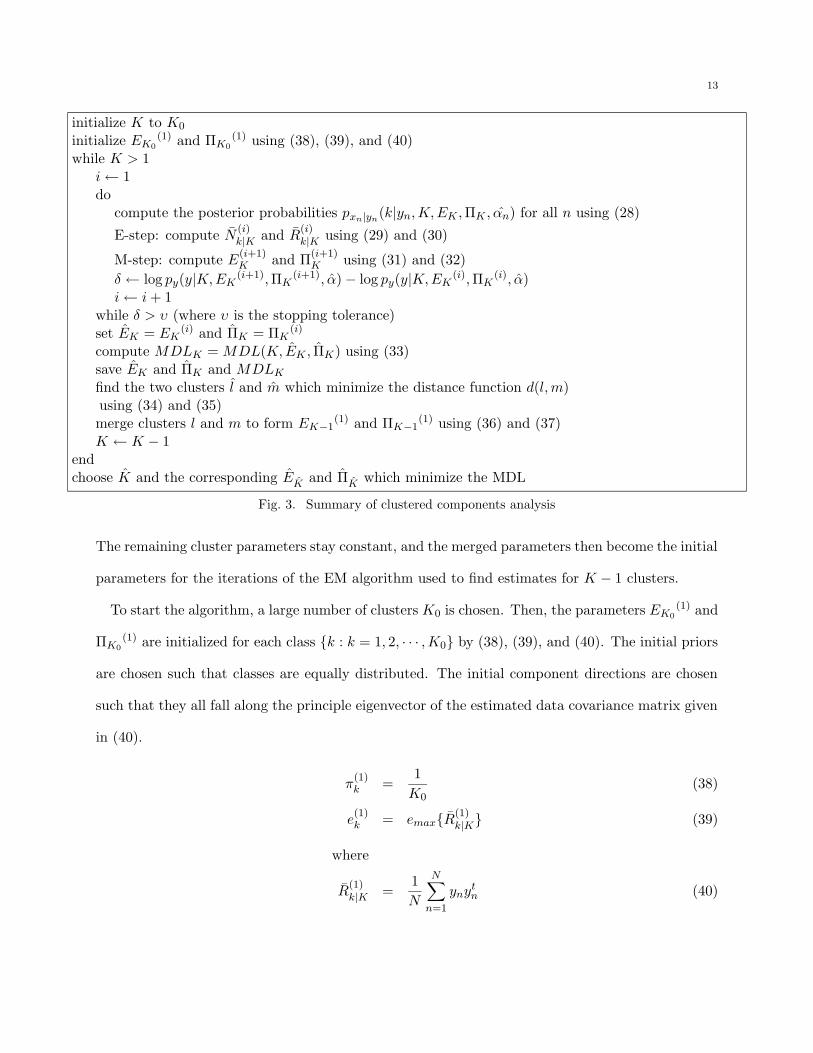
Fig. 3. Summary of clustered components analysis

The remaining cluster parameters stay constant, and the merged parameters then become the initial

parameters for the iterations of the EM algorithm used to find estimates for K − 1 clusters.

To start the algorithm, a large number of clusters K0 is chosen. Then, the parameters EK0(1) and

ΠK0(1) are initialized for each class {k : k = 1, 2, · · · , K0} by (38), (39), and (40). The initial priors

are chosen such that classes are equally distributed. The initial component directions are chosen

such that they all fall along the principle eigenvector of the estimated data covariance matrix given

in (40).

π(1)k =

1

K0(38)

e(1)k = emax{R

(1)k|K} (39)

where

R(1)k|K =

1

N

N∑

n=1

ynytn (40)

14

III. Methods

A. Experimental paradigm

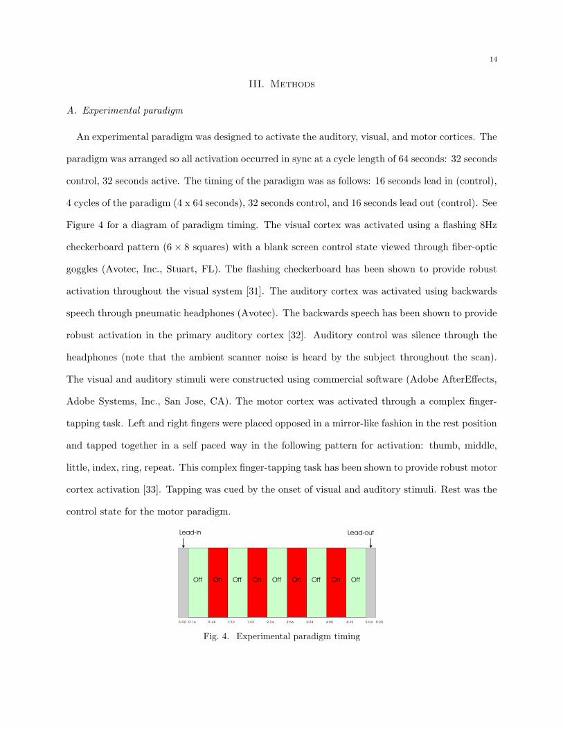
An experimental paradigm was designed to activate the auditory, visual, and motor cortices. The

paradigm was arranged so all activation occurred in sync at a cycle length of 64 seconds: 32 seconds

control, 32 seconds active. The timing of the paradigm was as follows: 16 seconds lead in (control),

4 cycles of the paradigm (4 x 64 seconds), 32 seconds control, and 16 seconds lead out (control). See

Figure 4 for a diagram of paradigm timing. The visual cortex was activated using a flashing 8Hz

checkerboard pattern (6 × 8 squares) with a blank screen control state viewed through fiber-optic

goggles (Avotec, Inc., Stuart, FL). The flashing checkerboard has been shown to provide robust

activation throughout the visual system [31]. The auditory cortex was activated using backwards

speech through pneumatic headphones (Avotec). The backwards speech has been shown to provide

robust activation in the primary auditory cortex [32]. Auditory control was silence through the

headphones (note that the ambient scanner noise is heard by the subject throughout the scan).

The visual and auditory stimuli were constructed using commercial software (Adobe AfterEffects,

Adobe Systems, Inc., San Jose, CA). The motor cortex was activated through a complex finger-

tapping task. Left and right fingers were placed opposed in a mirror-like fashion in the rest position

and tapped together in a self paced way in the following pattern for activation: thumb, middle,

little, index, ring, repeat. This complex finger-tapping task has been shown to provide robust motor

cortex activation [33]. Tapping was cued by the onset of visual and auditory stimuli. Rest was the

control state for the motor paradigm.

On OnOn On OnOff Off Off Off Off

Lead-in Lead-out

0:00 0:16 0:48 1:20 1:52 2:24 2:56 3:28 4:00 4:32 5:04 5:20

Fig. 4. Experimental paradigm timing

15

B. Human data acquisition

Whole-brain images of a healthy subject were obtained using a 1.5T GE Echospeed MRI Scanner

(GE Medical Systems, Waukeshau, WI). Axial 2D spin echo T1-weighted anatomic images were

acquired for reference with the following parameters: TE = 10ms TR = 500ms, matrix dimensions

= 256x128, 15 locations with thickness of 7.0 mm and gap of 2.0 mm covering the whole brain,

field-of-view = 24× 24 cm.

BOLD-weighted 2D gradient echo echoplanar imaging (EPI) functional images were acquired

during a run of the experimental paradigm with the following parameters: TE = 50ms, TR =

2000ms, flip angle = 90o, matrix dimensions= 64x64, 160 repetitions, and the same locations and

field-of-view as the anatomic images.

C. Synthetic data generation

To test the validity of the our methods, synthetic fMRI images were generated using the averaged

functional images gathered from the real data set acquired as per Section III-B as baseline images.

The BOLD response signals were modeled using the methods given by Purdon et al. [34], in the

three subsequent equations.

The physiologic model is based upon two gamma functions given by

ga(t) = (1− e−1/da)2(t + 1)e−t/da (41)

gb(t) = (1− e−1/db)e−t/db , (42)

where da and db are time constants. The activation signal s(t) is then a combination of these

gamma functions convolved (denoted by ∗) with the stimulus reference signal c(t) which equals 0

during the control states and 1 during the active states. d0 denotes a time delay and fa, fb, andfc

are amplitudes which characterize the activation.

s(t) = fa(ga ∗ c)(t− d0) + fb(gb ∗ c)(t− d0) +

fc(ga ∗ c)(t− d0)(gb ∗ c)(t− d0) (43)

The mixture weights, as well as time constant and time delay parameters, were varied between

16

TABLE I

Parameters used in synthetic data generation

Signal fa fb fc da db d0

1 0.6 0.02 0.2 1 10 22 0.35 0.2 0.5 3 5 83 0.35 0.1 1 5 5 15

three locations of 8× 8 in one slice in order to simulate responses from different functional cortices

and/or tissue characteristics. The parameters for (41), (42), and (43) are given in Table I for each

of the signals/locations.

The amplitudes of these signals were modulated by the baseline voxel intensities µn using 7% peak

activation and then multiplied by a normalized Gaussian window (G) (see Figure 5) to simulate

the variation in amplitudes across the functional region. Additive white Gaussian noise (ν) was

then added to all the voxels at a standard deviation of 2% of the mean baseline voxel intensity in

the entire brain.

yn(t) = µn + 0.07µnGnsn(t) + νn(t) (44)

12

34

56

78

0

2

4

6

80

0.2

0.4

0.6

0.8

1

Pixels in x directionPixels in y direction

Inte

nsity

wei

ghtin

g

Fig. 5. Gaussian window for variation in amplitude in the synthetic data. Each vertex in the meshcorresponds to a voxel in an 8 × 8 square region of interest. The mesh values at the vertices modulate theamplitudes of activation at the corresponding voxels.

17

D. Data processing

D.1 Synthetic data

In the synthetic data, only the voxels that had been injected with signal were considered for anal-

ysis. Mean and drift were removed from the voxel timecourses. Only the timepoints corresponding

to the first four cycles were considered (128 out of 160 time points). Because the sequence used

was a two-dimensional acquisition, each slice is acquired at staggered timing. Therefore, a dif-

ferent design matrix A was specified for each slice by shifting the harmonic components by the

corresponding time delay for the slice. The dimensionality reduction scheme including harmonic

decomposition and signal subspace estimation outlined in Section II-A was performed.

Principle components analysis (PCA) was applied to the synthetic data after harmonic decom-

position using the harmonic images Θ given in (4). An eigendecomposition was performed on Rsn

given in (11) to obtain the principle components. PCA was also applied to the synthetic data

after signal subspace estimation. The principle components are the columns of Us derived from

(14). In both cases, the three principle components were chosen corresponding to the three largest

variances.

Fuzzy C-means clustering (FCM), using the Matlab fuzzy toolbox (Mathworks, Natick, MA),

was also applied to the synthetic data on Θ and unwhitened feature vectors Y . The routine was

constrained to yield three clusters in both cases.

Spatial independent components analysis, using software available from [35], was applied to Θ

and to the Y . The analysis was applied unconstrained to yield as many components as channels

and also constrained to yield three independent components. For the unconstrained case, the three

independent components that best matched (in a least squares sense) the injected signals were

chosen.

Clustered components analysis was applied only after signal subspace estimation on the whitened

feature vectors Y . The CCA was initialized with K0 = 20 clusters. The resultant estimates were

transformed back into the time domain,

ek = ΣW−1ek, ∀k ∈ [1, · · · , K] (45)

18

in a manner similar to (17).

D.2 Human data

The functional image data were analyzed voxel-by-voxel for evidence of activation using a con-

ventional Student’s T-test analysis [21] using in-house software. Regions of interest were drawn

on the resulting statistical maps in the cortical regions corresponding to primary activated regions

for each of the three stimuli (i.e. precentral gyrus for the motor stimuli, superior temporal gyrus

for the auditory stimuli, and the calcarine fissure for the visual stimuli). Only the voxels in the

regions of interest were considered in the analysis. The data were processed for the dimensionality

reduction in the same manner as the synthetic data. CCA was applied to the resultant feature

vectors Y , and the results were transformed back into the time domain using (45). CCA for the

human data was also initialized with K0 = 20 clusters.

IV. Results

A. Synthetic Data

The harmonic decomposition and signal subspace estimation yielded L = 16 dimensions for the

synthetic data. The resultant signals from PCA, FCM, and ICA applied before and after signal

subspace estimation were then least squares fitted to each injected synthetic signal (peak-to-trough

amplitude normalized) and were matched by finding the combination with the smallest mean square

error per sample. The mean square error results of the analysis methods are shown in Table II.

The timesequence realizations are plotted for the analysis methods applied after signal subspace

estimation in Figure 6.

Hard classification results were then calculated by finding the largest membership value (e.g.,

largest component for PCA and ICA, largest membership value for FCM, and largest posterior

probability for CCA) for each voxel. The number of correct voxel classifications for the analyses is

shown in Table III. The hard classification results image for CCA is shown in Figure 7.

19

10 20 30 40 50 60 70 80 90 100 110

−0.5

0

0.5

10 20 30 40 50 60 70 80 90 100 110

−0.5

0

0.5

10 20 30 40 50 60 70 80 90 100 110

−0.5

0

0.5

10 20 30 40 50 60 70 80 90 100 110

−0.5

0

0.5

10 20 30 40 50 60 70 80 90 100 110

−0.5

0

0.5

10 20 30 40 50 60 70 80 90 100 110

−0.5

0

0.5

10 20 30 40 50 60 70 80 90 100 110

−0.5

0

0.5

10 20 30 40 50 60 70 80 90 100 110

−0.5

0

0.5

10 20 30 40 50 60 70 80 90 100 110

−0.5

0

0.5

(a) (b) (c)

10 20 30 40 50 60 70 80 90 100 110

−0.5

0

0.5

10 20 30 40 50 60 70 80 90 100 110

−0.5

0

0.5

10 20 30 40 50 60 70 80 90 100 110

−0.5

0

0.5

10 20 30 40 50 60 70 80 90 100 110

−0.5

0

0.5

10 20 30 40 50 60 70 80 90 100 110

−0.5

0

0.5

10 20 30 40 50 60 70 80 90 100 110

−0.5

0

0.5

(d) (e)

Fig. 6. Estimation methods after signal subspace estimation plotted against injected synthetic signal. (a)PCA, (b) FCM, (c) constrained ICA, (d) unconstrained ICA, (e) CCA. The solid blue estimated signals areleast squares fitted to the dotted red injected signals.

TABLE II

Mean squared error for analyses on synthetic data before and after signal subspace

estimation (SSE)

PCA FCM ICA (c) ICA (u) CCA

Before SSE 5.73×10−4 7.37×10−4 1.02×10−3 2.49×10−4 3.49×10−5

After SSE 5.80×10−4 1.95×10−4 2.21×10−4 1.63×10−4 3.09×10−5

TABLE III

Number of voxels classified correctly on synthetic data before and after signal

subspace estimation (SSE) out of 192 total voxels

PCA ICA (c) ICA (u) FCM CCA

Before SSE 61 113 38 95 167

After SSE 111 162 77 151 169

20

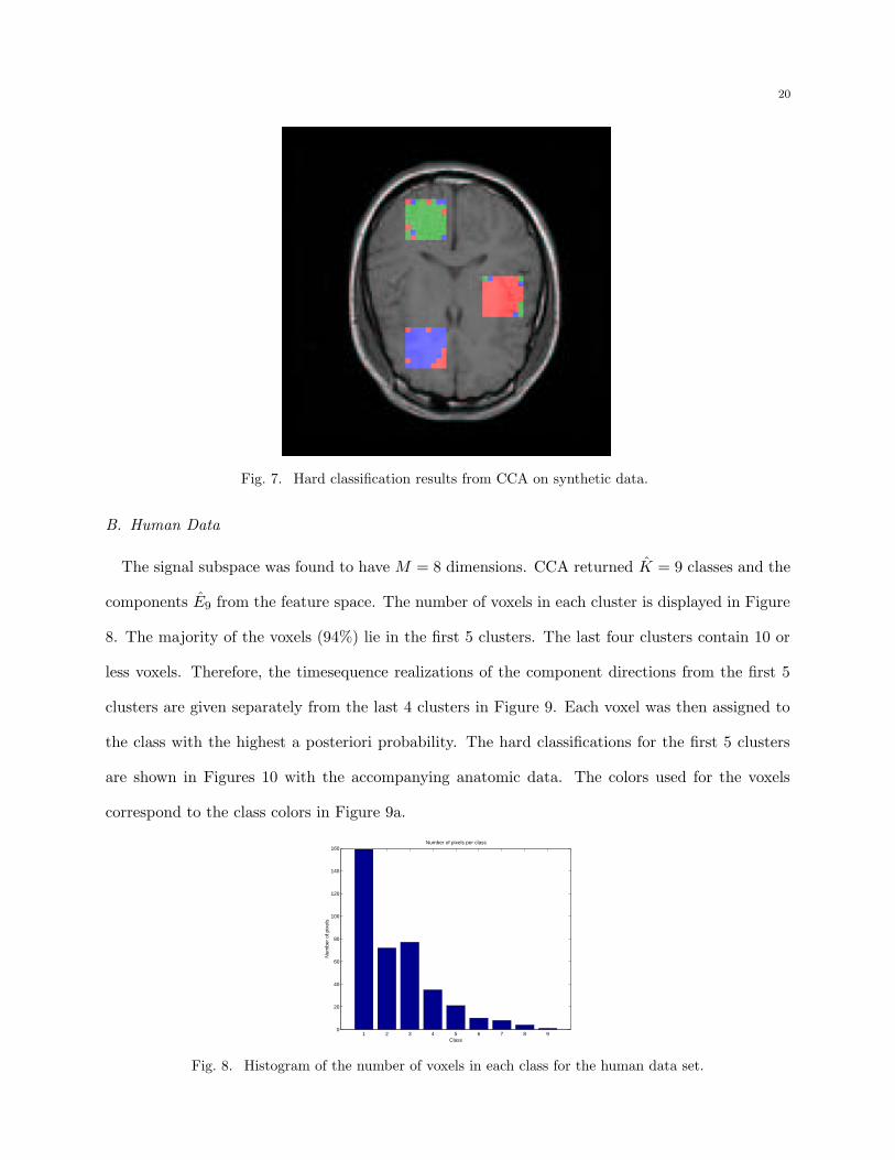
Fig. 7. Hard classification results from CCA on synthetic data.

B. Human Data

The signal subspace was found to have M = 8 dimensions. CCA returned K = 9 classes and the

components E9 from the feature space. The number of voxels in each cluster is displayed in Figure

8. The majority of the voxels (94%) lie in the first 5 clusters. The last four clusters contain 10 or

less voxels. Therefore, the timesequence realizations of the component directions from the first 5

clusters are given separately from the last 4 clusters in Figure 9. Each voxel was then assigned to

the class with the highest a posteriori probability. The hard classifications for the first 5 clusters

are shown in Figures 10 with the accompanying anatomic data. The colors used for the voxels

correspond to the class colors in Figure 9a.

1 2 3 4 5 6 7 8 90

20

40

60

80

100

120

140

160Number of pixels per class

Class

Num

ber

of p

ixel

s

Fig. 8. Histogram of the number of voxels in each class for the human data set.

21

20 40 60 80 100 120 140 160 180 200 220−2

−1.5

−1

−0.5

0

0.5

1

1.5

2Class 1Class 2Class 3Class 4Class 5

20 40 60 80 100 120 140 160 180 200 220−2

−1.5

−1

−0.5

0

0.5

1

1.5

2Class 6Class 7Class 8Class 9

(a) (b)

Fig. 9. Timesequence realizations of the feature space for the human data set. (a) Timesequences for thefirst 5 clusters, (b) timesequences for clusters 6-9

V. Discussion

A. Experimental results

Our simulation results show that, as a general rule, mean square error decreased by using signal

subspace estimation (except for PCA). The number of voxels classified correctly increased for each

analysis method as a result of signal subspace estimation. It can also be seen that CCA outperforms

each of the other analysis methods in both mean square error and correct voxel classification.

Although in CCA the changes are small before and after signal subspace estimation in both mean

square error and correct classification, the signal subspace estimation speeds the algorithm greatly.

The experimental results from the human data reveal that a distinct functional behavior does

not correlate directly with each of the functional ROIs, at least for the motor and auditory cortices.

Inspection of Figure 10 shows that the classes are distributed along patterns of location with

respect to sulcal-gyral boundaries. This may reflect that the temporal evolution of the BOLD

signal is dependent much more on the vascularization of the tissue than the functional specifics of

neuronal activation.

B. Relation to other analysis methods

In this paper, we have attempted to develop an analysis framework that incorporates the advan-

tages of previous methods. This section will detail how our methods relate to other multivariate

22

50 100 150 200 250

50

100

150

200

250

50 100 150 200 250

50

100

150

200

250

50 100 150 200 250

50

100

150

200

250

(a) (b) (c)

50 100 150 200 250

50

100

150

200

250

50 100 150 200 250

50

100

150

200

250

50 100 150 200 250

50

100

150

200

250

(d) (e) (f)

Fig. 10. CCA hard classification on the real data set (first 5 clusters) The colors correspond to the classcolors shown in Figure 9a. (a) upper motor cortex slice, (b) upper auditory cortex slice, (c) - upper visualcortex slice, (d) lower motor cortex slice, (e) lower auditory cortex slice, and (f) - lower visual cortex slice

methods used by other researchers. We note that over the past few years some commonly used

algorithms for analyzing fMRI data have been widely distributed as software packages [36], [37].

Linear time invariant systems methods try to model the hemodynamic impulse response function

by using deconvolution. Although it has been shown that for some cases linearity is reasonable [11],

[12], for other situations nonlinearities arise [38]. Parametric methods are heavily model driven and

not as suitable if data are not described well by the model. Therefore, data-driven methods should

be used in fMRI where the mechanisms of the system are unknown. Our approach is data-driven

and may be more appropriate in this case.

PCA is a method which uses the eigenanalysis of signal correlations to produce orthogonal

components in the directions of maximal variance [39], [40]. However, it is unlikely that the distinct

23

behaviors in fMRI data correspond to orthogonal signals. Backfrieder et al. [14], attempted to solve

this problem by using an oblique rotation of the components. Most researchers, however, use PCA

as a preprocessing step for dimensionality reduction. A threshold is usually arbitrarily set to the

number of components kept [13]. We use a method similar to PCA for dimensionality reduction.

Our threshold, however, is determined from the data itself after noise covariance estimation from

harmonic decomposition and should effectively remove this subjective aspect the analysis.

ICA is used in signal processing contexts to separate out mixtures of independent sources or invert

the effects of an unknown transformation [41]. It was adapted to produce spatial independent

components for fMRI datasets by McKeown et al. [15], [16]. The fMRI data is modeled as a

linear combination of maximally independent (minimally overlapping) spatial maps with component

timecourses. It has been pointed out, however, that neuronal dynamics may overlap spatially [42].

Our method does not constrain distinct behaviors to be spatially independent. Another shortcoming

of ICA is that it does not lend itself to statistical analysis. McKeown and Sejnowski have attempted

to solve this problem by developing a method to calculate the posterior probability of observing

a voxel timecourse given the ICA unmixing matrix [43]. Because CCA is based upon an explicit

statistical model, it does not suffer from this disadvantage.

Clustering algorithms have been applied to both fMRI raw timecourse data [18], [20], [44] and

to timecourse features such as univariate statistics and correlations [45]. Because we are trying to

estimate the response signal, we use a hybrid method to characterize the timecourses into lower

dimensionality representations. The main problem with most of these clustering methods is that the

variation in amplitude is not taken into consideration. Our method produces component directions

due to the amplitude variances (see Figure 1) rather than traditional cluster means. More recently,

Brankov et al. [46], proposed an alternative clustering approach which is also designed to account

for variations in signal amplitude. Another shortcoming of most clustering methods is that the

number of clusters is arbitrarily determined. Baune et al. [20], attempt to solve this problem by

setting a threshold on Euclidean distances for the merging of clusters. Liang et al. [30], also used

an information criterion for order identification (AIC and MDL) to analyze PET and SPECT data

24

to find image parameters. Our method uses the MDL criterion plus a cluster merging strategy to

determine the number of clusters in an unsupervised manner.

C. Algorithm details

We use a design matrix A which consists of harmonic components used in the dimensionality

reduction applied in this paper. Periodicity of the response signal is assumed due to the block

design of the stimulus paradigm. This assumption allows for the reduction in dimensionality and

the estimation of a noise covariance for signal subspace estimation. However, periodicity is not

a trait of all stimulus paradigms. In non-periodic paradigm designs, the CCA method can still

be applied without the SSE step. It can be seen in Tables II and III that CCA performs well

even without SSE. Other orthogonal bases, including wavelets and splines, may also be used as

the design matrix. These may also allow for estimation of a noise covariance, but we have not

explored the details of this approach. CCA can even be applied to event-related approaches where

the inter-stimulus interval is random.

In this paper, the assumption is made that the noise in the images is additive white Gaussian.

It is known, in fact, that the noise in magnitude MRI data is Rician [47]. In addition, in dynamic

in-vivo MR imaging, physiologic processes introduce correlated “noise.” However, as a first order

approximation, the additive white Gaussian noise model works fairly well. The framework we have

presented can be generalized to more complex noise models.

Because the two steps of our method are both entirely self-sufficient, they can be used indepen-

dently of each other. The SSE methods of the first step can be used in conjunction with multivariate

clustering methods other than our CCA. Conversely, the CCA can be used on any dataset which

contain feature vectors which have the property of amplitude variation which we discussed in Sec-

tion I. As a generalization, these methods can also be used in applications outside the realm of

fMRI.

25

VI. Conclusion

In this paper, we have introduced two novel ideas for the analysis of fMRI timeseries data. The

first was a method to reduce the dimensionality and increase SNR by using a signal subspace

estimation and simple thresholding strategy. The second was the method of clustered components

analysis in which the data were iteratively classified independent of signal amplitude. The second

method also included a technique to find the number of clusters in an unsupervised manner.

The methodology presented here will allow investigators to improve the estimation of the BOLD

signal response by dramatically improving SNR through signal averaging without destroying po-

tentially important statistically distinct temporal elements in the process.

Appendix

I. Derivation of noise covariance

In this appendix, we derive an estimate for the noise covariance matrix of the noise subspace.

Using (7), and defining the matrix PA = A(AtA)−1At results in the relation ε = (I − PA)ν. Using

the assumption that the noise is white, we have Iσ2 = 1N E

[

ννt]

, where I is an identity matrix and

σ is the variance of the noise. From this we know that σ2 = 1NP E

[

tr{

ννt}]

. Using these results,

we derive the following.

E[

tr{

εεt}]

= σ2E[

tr{

(I − PA)ννt(I − PA)t}]

= σ2tr{

(I − PA)E[

ννt]

(I − PA)t}

= σ2Ntr{

(I − PA)(I − PA)t}

= σ2N(P − L− 2)

The noise covariance matrix may then be computed.

Rn =1

NE[

ΘΘt]

=1

N(AtA)−1AtE

[

ννt]

A(AtA)−1

= σ2(AtA)−1AtA(AtA)−1

= E[

tr{εεt}]

(AtA)−1/(N(P − L− 2))

26

= E[

Rn

]

,

where Rn is given in (12).

II. Derivation of Whitening Matrix

The corrected noise covariance matrix after subspace processing is denoted as Rn where

Rn = U tsRnUs . (46)

The whitening filter matrix W has the property that R−1n = WW t. Let Rn = UnSnV t

n be the

singular value decomposition where Sn is a diagonal matrix of singular values. Then, the whitening

matrix is is given by

W = Vn

[

√

Sn

]−1, (47)

and the whitened feature vectors are given by Y = WY .

III. Expectation-Maximization Algorithm

A. Expectation step

The Q function used in the EM algorithm is defined as the expectation of the joint log-likelihood

function given the current estimates of the parameters. Knowing this, we can write

Q(K, EK , ΠK ; E(i)K , Π

(i)K )

= Ex|y[log py,x(y, X|EK , ΠK , α)|y, K, E(i)K , Π

(i)K , α] (48)

=K∑

k=1

[

log py|x(y|k, EK , ΠK , α) log px(k|ΠK)]

px|y(k|y, E(i)K , Π

(i)K , α). (49)

Because of conditional independence, the one-to-one mapping of xn → yn, and px(k|ΠK) = πk,

Q(K, EK , ΠK ; E(i)K , Π

(i)K ) =

K∑

k=1

{

N∑

n=1

[

−1

2

(

ytnyn − et

kynytnek

)

pxn|yn(k|yn, E

(i)K , Π

(i)K , α)

]

−M − 1

2log(2π)

N∑

n=1

pxn|yn(k|yn, E

(i)K , Π

(i)K , α) + log πk

N∑

n=1

pxn|yn(k|yn, E

(i)K , Π

(i)K , α)

}

(50)

Now define

N(i)k|K =

N∑

n=1

pxn|yn(k|yn, E

(i)K , Π

(i)K , α) (51)

27

and

R(i)k|K =

1

Nk|K

N∑

n=1

ynytnpxn|yn

(k|yn, E(i)K , Π

(i)K , α) . (52)

We can then write the Q function in its final form.

Q(K, EK , ΠK ; E(i)K , Π

(i)K )

=K∑

k=1

N(i)k|K

{

−1

2tr(R

(i)k|K) +

1

2etkR

(i)k|Kek −

M − 1

2log(2π) + log πk

}

(53)

B. Maximization step

In order to find E(i+1), we maximize Q with respect to each ek, k ∈ {1, 2, ..., K}. We can see that

all the terms are constant with respect to ek except 12et

kR(i)k|Kek. So maximizing this factor with

respect to ek is equivalent to maximizing Q. The update equation becomes

e(i+1)k = argmax

ek

(

etkR

(i)k|Kek

)

. (54)

It is known from linear algebra theory that the solution to this maximization is the principle

eigenvector of R(i)k|K . If we let emax(R) be the principle eigenvector of R, we can write the update

equation as

e(i+1)k = emax(R

(i)k|K) . (55)

Now we need to find Π(i+1)K . We can see that all the terms of Q are constant with respect to each

πk except for N(i)k|K log πk. Therefore, maximizing this term with respect to πk is equivalent to

maximizing Q with respect to πk. The problem is a constrained optimization because∑K

k=1 πk = 1

due to the fact that these are probabilities. If the method of Lagrange multipliers is applied, we

find that the update equations for ΠK(i+1).

π(i+1)k =

N(i)k|K

N(56)

IV. Derivation of Cluster Merging

In this section, we derive the distance function used for cluster merging in minimization of the

MDL criterion. Let l and m denote the indices of the two clusters to be merged. Let EK and

ΠK to be the result of running the EM algorithm to convergence with clusters of order K, and let

28

E(l,m)|K and Π(l,m)|K denote new parameter sets in which the parameters for clusters l and m are

equated. This means that Π(l,m)|K = ΠK and E(l,m)|K remains the same except for the column

vectors corresponding to the clusters l and m which are modified to be

el = em = e(l,m) (57)

where e(l,m) denotes the common value of the parameter vectors.

Also define the subscript E(l,m)|K−1 and Π(l,m)|K−1 to be parameter sets with K − 1 clusters

in which the l and m clusters have been merged into a single cluster with parameters e(l,m) and

π(l,m) = πl + πm. The change in the MDL criterion produced by merging the clusters l and m is

then given by

MDL(K − 1, E(l,m)|K−1, Π(l,m)|K−1)−MDL(K, EK , ΠK)

= MDL(K − 1, E(l,m)|K−1, Π(l,m)|K−1)−MDL(K, E(l,m)|K , Π(l,m)|K)

+ MDL(K, E(l,m)|K , Π(l,m)|K)−MDL(K, EK , ΠK) (58)

From (33), we can see that

MDL(K − 1, E(l,m)|K−1, Π(l,m)|K−1)−MDL(K, E(l,m)|K , Π(l,m)|K) = −M

2log(NM) ; (59)

and from the upper bounding properties of the Q-function, we know that

MDL(K, E(l,m)|K , Π(l,m)|K)−MDL(K, EK , ΠK)

≤ Q(K, EK , ΠK ; EK , ΠK)−Q(K, E(l,m)|K , Π(l,m)|K ; EK , ΠK) . (60)

Substituting into (58) results the following inequality.

MDL(K − 1, E(l,m)|K−1, Π(l,m)|K−1)−MDL(K, EK , ΠK)

≤ Q(K, EK , ΠK ; EK , ΠK)−Q(K, E(l,m)|K , Π(l,m)|K ; EK , ΠK)−M

2log(NM) (61)

Since we assume that EK and ΠK are the result of running the EM algorithm to convergence,

we know that

(EK , ΠK) = argmaxE′

K,Π′

K

Q(K, E′K , Π′

K ; EK , ΠK) . (62)

29

Furthermore, the inequality of (58) is most tight when E(l,m)|K and Π(l,m)|K are chosen to be

(E(l,m)|K , Π(l,m)|K) = argmaxE′

(l,m)|K,Π′

(l,m)|K

Q(K, E′(l,m)|K , Π′

(l,m)|K ; EK , ΠK) . (63)

The optimization of (63) is a constrained version of (62). It is easily shown that values of

(E(l,m)|K , Π(l,m)|K) and (EK , ΠK) are equal except for the parameter vector e(l,m) which is given

by

e(l,m) = emax{Rl|K + Rm|K}, (64)

where emax{R} is the principle eigenvector of R, and Rl|K and Rm|K are computed using (30).

Substituting into (61) and simplifying the expression for the Q function results in

MDL(K − 1, E(l,m)|K−1, Π(l,m)|K−1)−MDL(K, EK , ΠK)

≤ Q(K, EK , ΠK ; EK , ΠK)−Q(K, E(l,m)|K , Π(l,m)|K ; EK , ΠK)−M

2log(NM)

= σmax(Rl|K) + σmax(Rm|K)− σmax(Rl|K + Rm|K)−M

2log(NM) (65)

which produces the final result

MDL(K − 1, E(l,m)|K , Π(l,m)|K)−MDL(K, EK , ΠK) ≤ d(l, m)−M

2log(NM) (66)

where d(l, m) is the positive distance function in (34).

Acknowledgments

The authors would like to thank Brian Cook for help in the development of the stimulus paradigm

and Julie Lowe for help in scanning.

References

[1] S. Ogawa, T. M. Lee, A. R. Kay, and D. W. Tank, “Brain magnetic resonance imaging with contrast dependenton blood oxygenation,” Proc. Natl. Acad. Sciences, vol. 87, pp. 9868–9872, 1990.

[2] K. K. Kwong, J. W. Belliveau, D. A. Chesler, I. E. Goldberg, R. M. Weisskoff, B. P. Poncelet, D. N. Kennedy,B. E. Hoppel, M. S. Cohen, R. Turner, H. Cheng, T. J. Brady, and B. R. Rosen, “Dynamic magnetic resonanceimaging of human brain activity during primary sensory stimulation,” Proc. Natl. Acad. Sciences, vol. 89, pp.5675–5679, 1992.

[3] J. W. Belliveau, D. N. Kennedy, R. C. McKinstry, B. R. Buchbinder, R. M. Weisskoff, M. S. Cohen, J. M. Vevea,T. J. Brady, and B. R. Rosen, “Functional mapping of the human visual cortex by magnetic resonance imaging,”Science, vol. 254, pp. 716–719, 1991.

[4] P. A. Bandettini, E. C. Wong, , R. S. Hinks, R. S. Tikofsky, and J. S. Hyde, “Time course EPI of human brainfunction during task activation,” Magnetic Resonance in Medicine, vol. 25, pp. 390–397, 1992.

30

[5] P. A. Bandettini, A. Jesmanowicz, E. C. Wong, and J. S. Hyde, “Processing strategies for time-course data setsin functional MRI of the human brain,” Magnetic Resonance in Medicine, vol. 30, pp. 161–173, 1993.

[6] K. J. Friston, P. Jezzard, and R. Turner, “Analysis of functional MRI time-series,” Human Brain Mapping, vol.2, pp. 69–78, 1994.

[7] G. M. Hathout, S. S. Gambhir, R. K. Gopi, K. A. Kirlew, Y. Choi, G. So, D. Gozal, R. Harper, R. B. Lufkin,and R. Hawkins, “A quantitative physiologic model of blood oxygenation for functional magnetic resonanceimaging,” Investigative Radiology, vol. 30, no. 11, pp. 669–682, November 1995.

[8] R. B. Buxton, E. C. Wong, and L. R. Frank, “Dynamics of blood flow and oxygenation changes during brainactivation: the balloon model,” Magnetic Resonance in Medicine, vol. 39, pp. 855–864, 1998.

[9] F. Kruggel and D. Y. von Cramon, “Temporal properties of the hemodynamic response in functional MRI,”Human Brain Mapping, vol. 8, pp. 259–271, 1999.

[10] V. Solo, P. Purdon, R. Weisskoff, and E. Brown, “A signal estimation approach to functional MRI,” IEEE

Trans. on Medical Imaging, vol. 20, no. 1, pp. 26–35, January 2001.[11] G. M. Boynton, S. A. Engel, G. H. Glover, and D. J. Heeger, “Linear systems analysis of functional magnetic

resonance imaging in human V1,” J. of Neuroscience, vol. 16, no. 13, pp. 4207–4221, 1996.[12] M. S. Cohen, “Parameteric analysis of fMRI data using linear systems methods,” Neuroimage, vol. 6, pp. 93–103,

1997.[13] J. J. Sychra, P. A. Bandettini, N. Bhattacharya, and Q. Lin, “Synthetic images by subspace transforms I.

Principal components images and related filters,” Medical Physics, vol. 21, no. 2, pp. 193–201, February 1994.[14] W. Backfrieder, R. Baumgartner, M. Samal, E. Moser, and H. Bergmann, “Quatification of intensity variations

in functional MR images using rotated principal components,” Physics in Medicine and Biology, vol. 41, pp.1425–1438, 1996.

[15] M. J. McKeown, S. Makeig, G. G. Brown, T.-P. Jung, S. S. Kindermann, A. J. Bell, and T. J. Sejnowski,“Analysis of fMRI data by blind separation into independent spatial components,” Human Brain Mapping, vol.6, pp. 160–188, 1998.

[16] M. J. McKeown, T-P Jung, S. Makeig, G. Brown, S. S. Kindermann, T-W Lee, and T. J. Sejnowski, “Spatiallyindependent activity patterns in functional MRI data during the Stroop color-naming task,” Proc. Natl. Acad.

Sciences, vol. 95, pp. 803–810, 1998.[17] C. Goutte, P. Toft, E. Rostrup, F. A. Nielsen, and L. K Hansen, “On clustering fMRI time series,” Neuroimage,

vol. 9, pp. 298–310, 1999.[18] K-H Chuang, M-J Chiu, C-C Lin, and J-H Chen, “Model-free functional MRI analysis using Kohonen clustering

neural network and fuzzy c-means,” IEEE Trans. on Medical Imaging, vol. 18, no. 12, pp. 1117–1128, December1999.

[19] X. Golay, S. Kollias, G. Stoll, D. Meier, A. Valvanis, and P. Boesiger, “A new correlation-based fuzzy logicclustering algorithm for fMRI,” Magnetic Resonance in Medicine, vol. 40, pp. 249–260, 1998.

[20] A. Baune, F. T. Sommer, M. Erb, D. Wildgruber, B. Kardatzki, Palm, and Grodd, “Dynamical cluster analysisof cortical fMRI activation,” Neuroimage, vol. 9, pp. 477–489, 1999.

[21] M. J. Lowe and D. P. Russell, “Treatment of baseline drifts in fMRI time series analysis,” J. of Computer

Assisted Tomography, vol. 23, no. 3, pp. 463–473, 1999.[22] E. T. Bullmore, S. Rabe-Hesketh, R. G. Morris, L. Gregory S. C. R. Williams, J. A. Gray, and M. J. Brammer,

“Function magnetic resonance image analysis of a large-scale neurocognitive network,” Neuroimage, vol. 4, no.1, pp. 16–33, August 1996.

[23] S. Chen, C. A. Bouman, and M. J. Lowe, “Harmonic decomposition and eigenanalysis of BOLD fMRI timeseriesdata in different functional cortices,” in Proc. of the ISMRM Eighth Scientific Meeting, Denver, April 3-7 2000,p. 817.

[24] B.A. Ardekani, J. Kershaw, K. Kashikura, and I. Kanno, “Activation detection in functional MRI using subspacemodeling and maximum likelihood estimation,” IEEE Trans. on Medical Imaging, vol. 18, no. 2, pp. 101–114,1999.

[25] A. F. Sole, S.-C. Ngan, G. Sapiro, X. Hu, and A. Lopez, “Anisotropic 2-D and 3-D averaging of fMRI signals,”IEEE Trans. on Medical Imaging, vol. 20, no. 2, pp. 86–93, February 2001.

[26] A. P. Dempster, N. M. Laird, and D. B. Rubin, “Maximum likelihood from incomplete data via the EMalgorithm,” Journal of the Royal Statistical Society B, vol. 39, no. 1, pp. 1–38, 1977.

[27] E. Redner and H. Walker, “Mixture densities, maximum likelihood and the EM algorithm,” SIAM Review, vol.26, no. 2, April 1984.

[28] J. Rissanen, “A universal prior for integers and estimation by minimum description length,” The Annals of

Statistics, vol. 11, no. 2, pp. 417–431, September 1983.[29] C. A. Bouman, “Cluster: an unsupervised algorithm for modeling Gaussian mixtures,” Available from

http://www.ece.purdue.edu/˜bouman, April 1997.

31

[30] Z. Liang, R. J. Jaszczak, and R. E. Coleman, “Parameter estimation of finite mixtures using the EM algorithmand information criteria with applications to medical image processing,” IEEE Trans. on Nuclear Science, vol.39, no. 4, pp. 1126–1133, 1992.

[31] M. J. Lowe, M. Dzemidzic, J. T. Lurito, V. P. Mathews, and M. D. Phillips, “Functional discrimination ofthalamic nuclei using BOLD contrast at 1.5T,” in Proc. of the ISMRM Eighth Scientific Meeting, Denver, April3-7 2000, p. 888.

[32] M. D. Phillips, M. J. Lowe, J. T. Lurito, M. Dzemidzic, and V. P. Matthews, “Temporal lobe activationdemonstrates sex-based differences during passive listening,” Radiology, vol. 220, no. 1, pp. 202–207, July 2001.

[33] M. J. Lowe, J. T. Lurito, V. P. Matthews, M. D. Phillips, and G. D. Hutchins, “Quantitative comparison offunctional contrast from BOLD-weighted spin-echo and gradient-eco echoplanar imaging at 1.5T and H2

150PET in the whole brain,” J. of Cerebral Blood Flow and Metabolism, vol. 20, no. 9, pp. 1331–40, September2000.

[34] P. Purdon, V. Solo, E. M. Brown, and R. Weisskoff, “Functional MRI signal modeling with spatial and temporalcorrelations,” Neuroimage, vol. 14, no. 4, pp. 912–923, Oct 2001.

[35] S. Makeig, “EEG/ICA toolbox for Matlab,” Available from http://www.sccn.ucsd.edu/˜scott/ica.html, Septem-ber 2001.

[36] K. J. Friston, A. P. Holmes, K. J. Worsley, J. P. Poline, C. D. Frith, and R. S. J. Frackowiak, “Statisticalparametric maps in functional imaging: A general linear approach,” Human Brain Mapping, vol. 2, pp. 189–210,1995.

[37] R. W. Cox, “Afni: Software for analysis and visualization of functional magnetic resonance neuroimages,”Computers and Biomedical Research, vol. 29, pp. 162–173, 1996.

[38] A. L. Vazquez and D. C. Noll, “Nonlinear aspects of the BOLD response in functional MRI,” Neuroimage, vol.7, pp. 108–118, 1998.

[39] R. A. Johnson and D. W. Wichern, Applied Multivariate Statistical Analysis, 4th ed., Prentice-Hall, Inc., UpperSaddle, NJ, 1998.

[40] K. J. Friston, C. D. Frith, P. F. Liddle, and R. S. Frackowiak, “Functional connectivity: The principal-componentanalysis of large (PET) data sets,” J. of Cerebral Blood Flow and Metabolism, vol. 13, no. 1, pp. 5–14, 1993.

[41] A. J. Bell and T. J. Sejnowski, “An information maximization approach to blind separation and blind deconvo-lution,” Neural Computation, vol. 7, pp. 1129–1159, 1995.

[42] K. J. Friston, “Modes or models: a critique on independent component analysis for fMRI,” Trends in cognitive

sciences, vol. 2, no. 10, pp. 373–375, October 1998.[43] M. J. McKeown and T. J. Sejnowski, “Independent component analysis of fMRI data: Examining the assump-

tions,” Human Brain Mapping, vol. 6, pp. 368–372, 1998.[44] R. Baumgartner, C. Windischberger, and E. Moser, “Quantification in functional magnetic resonance imaging:

Fuzzy clustering vs. correlation analysis,” Magnetic Resonance Imaging, vol. 16, no. 2, pp. 115–125, 1998.[45] C. Goutte, L. K. Hansen, M. G. Liptrot, and E. Rostrup, “Feature-space clustering for fMRI meta-analysis,”

Human Brain Mapping, vol. 13, pp. 165–183, 2001.[46] J. G. Brankov, N. P. Galatsanos, Y. Yang, and M. N. Wernick, “Similarity based clustering using the expectation

maximization algorithm,” in Proc. of IEEE Int’l Conf. on Image Proc., Rochester, September 22-25 2002, p. to

appear.[47] J. Sijbers, A. J. den Dekker, J. Van Audekerke, M. Verhoye, and D. Van Dyck, “Estimation of the noise in

magnitude MR images,” Magnetic Resonance Imaging, vol. 16, no. 1, pp. 87–90, 1998.