1

Blind Separation of Audio Mixtures Using Direct Estimation of Delays

Arie YeredorDept. of Elect. Eng. – SystemsSchool of Electrical EngineeringTel-Aviv University

2

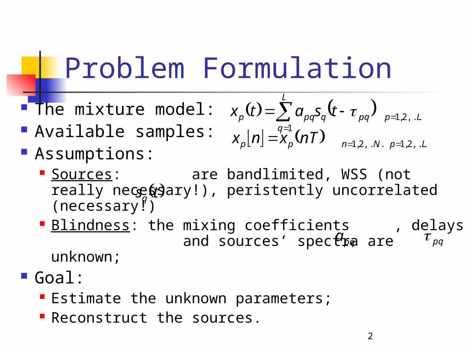
Problem Formulation The mixture model: Available samples: Assumptions:

Sources: are bandlimited, WSS (not really necessary!), peristently uncorrelated (necessary!)

Blindness: the mixing coefficients , delays and sources’ spectra are unknown;

Goal: Estimate the unknown parameters; Reconstruct the sources.

Lp

L

qpqqpqp tsatx ,...2,1

1

tsq

pqa pq

LpNnpp nTxnx ,...2,1,...2,1

3

Falling between the chairs

Static BSS is obviously under-parameterized;

Convolutive BSS is not only over-parameterized, but also inappropriate for accommodating fractional delays, especially with FIR models.

4

Inherent ambiguities

Sources’ scaling assume normalized power

Sources’ time-origin assume

Sources’ permutation assume we don’t care

Lppp ,...2,10

5

Mixtures’ correlations

The mixtures’ correlations are given by

L

qnqmq

L

p

L

qnqqmppnqmp

nm

aa

tstsEaa

txtxE

1

1 1

xmnR

mqnqsqR

6

Mixtures’ spectra Fourier-transforming the correlations:

or

with

is the mixing matrix

contains freq.-domain delays:

denotes Hadamard (element-wise) product

xmnS

L

q

nqmqnqmq

jeaa1

sqS

HBB xS sS

DAB

A

D mnmn

jeD

7

Estimate mixtures’ spectra Use, e.g., Blackman-Tukey estimates:

with

where is some rough upper-bound on the correlations length of all sources.

The frequency axis is rescaled to the range ,thus the delays are normalized to units of .

xmnS

M

M

je

xmnR

MM

N

pnmNxpx

1

1 xmnR

M

:T

8

Obtain a frequency-dependent joint-diagonalization problem

Use a selected set of frequencies , and attempt to jointly diagonalize the estimated spectral matrices

by minimizing w.r.t: the mixing parameters; the delays; the respective sources’ spectra: .

1K

K ,..., 10

A

T

Γ ksmkmk S Γ

LSC

K

kFk

HkLSC

0

2min,, BBTA ˆ

x kS ks SΓ

9

Extended AC-DC Use an extended veriosn of the

“Alternating Columns - Diagonal Centers” (AC-DC, Yeredor, ’02) algorithm for the joint diagonalization:

Alternate between minimizations w.r.t.: (in the DC phase) each column of (in the AC-1 phase) each column of (in the AC-2 phase)

In each phase all other parameters are assumed fixed.

ΓAT

10

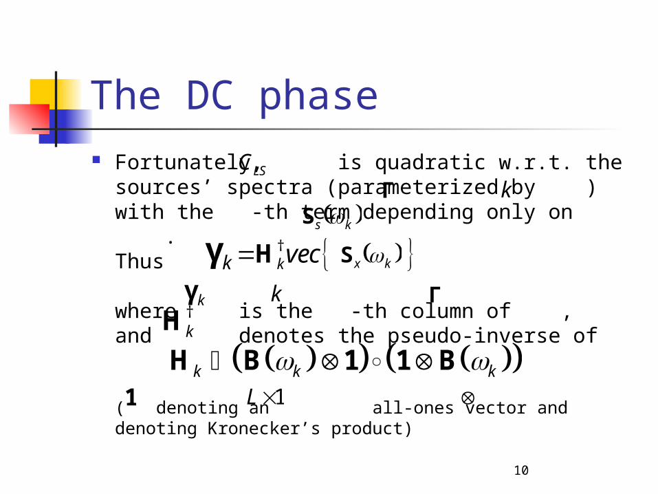
The DC phase Fortunately, is quadratic w.r.t. the sources’

spectra (parameterized by ) with the -th term depending only on .Thus

where is the -th column of ,and denotes the pseudo-inverse of

( denoting an all-ones vector and denoting Kronecker’s product)

LSCΓ k

ks S

kkγ Γ†kH

k k k H B 1 1 B

†kvecH kx Skγ

1 1L

11

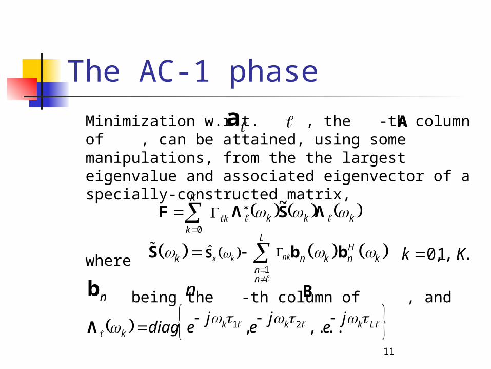
The AC-1 phase

Minimization w.r.t. , the -th column of , can be attained, using some manipulations, from the the largest eigenvalue and associated eigenvector of a specially-constructed matrix,

where

being the -th column of , and

kK

kkk ΛSΛF

0

~

Aa

1

LH

k n k n knn

S b b

ˆx kS nk

nb n B

Kk ,..1,0

Lkkkk

je

je

jediag

,..., 21Λ

k

12

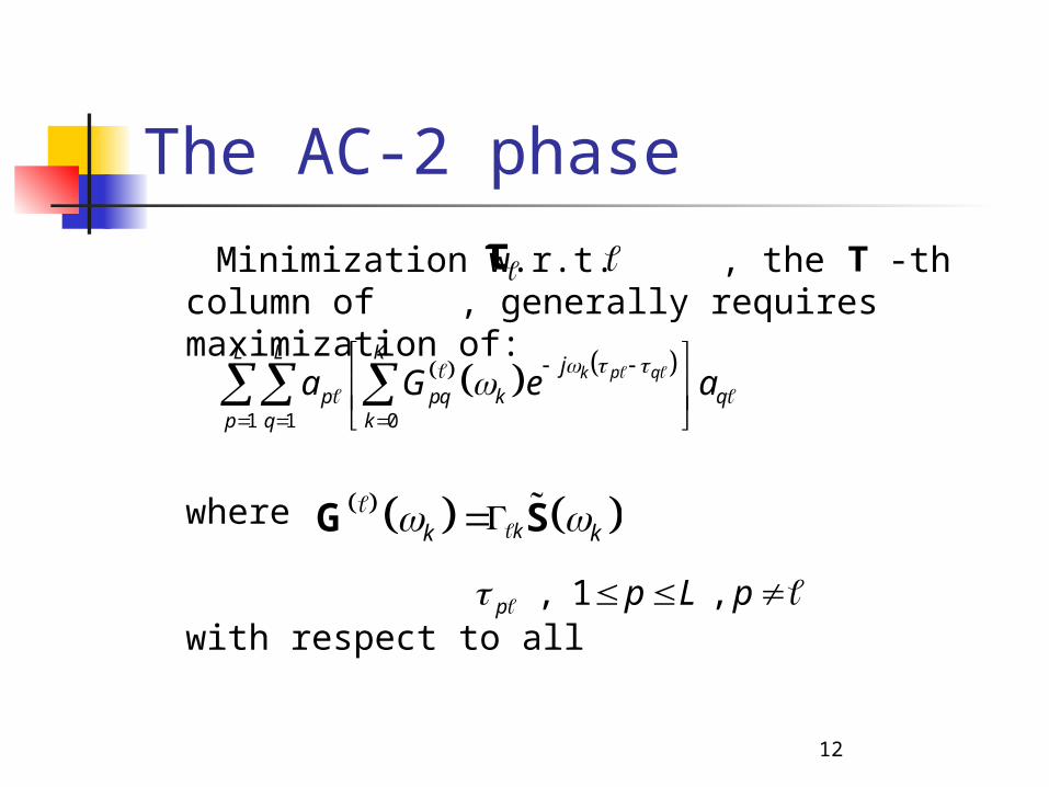
The AC-2 phase

Minimization w.r.t. , the -th column of , generally requires maximization of:

where

with respect to all

τ T

k k G S k

pLpp ,1,

1 1 0

p qkL L K

p pq k qp q k

ja G e a

13

The AC-2 phase (cont’d) For the case this maximization

translates into a simple line-search (for each ), maximizing:

In addition, in this case the maximization only depends on the sign of elements of , which means that effectively the AC-2 phase is almost always an integral part of the AC-1 phase.

2L

111 21 12 21

0

max Re k

K

kk

ja a G e

A

222 12 21 21

0

max Re k

K

kk

ja a G e

14

Reconstruction of the sources

Comfortable reconstruction in the frequency domain:

Compute the observations’ DFTs:

where and

0,1,... 1

1

2 1 /N

m Nn

j n m Nm n e

y x

1 2

T

Ln x n x n x n x 1 2

T

Lm y m y m y m y

15

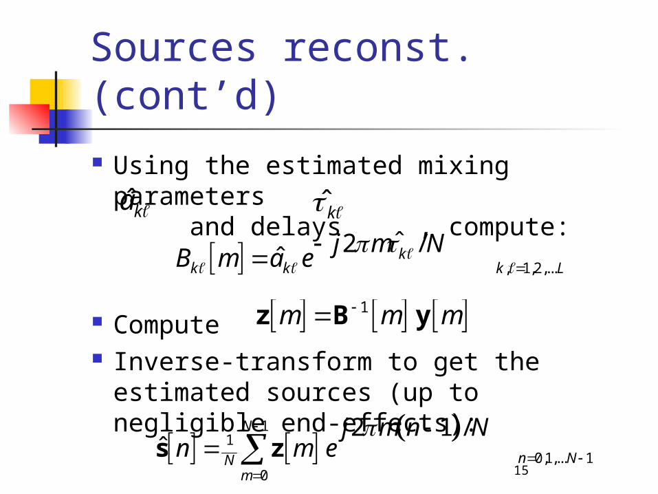
Sources reconst. (cont’d)

Using the estimated mixing parameters and delays , compute:

Compute Inverse-transform to get the estimated

sources (up to negligible end-effects):

ka k

, 1,2,...

ˆ2 /ˆ kk k k L

j m NB m a e

1m m mz B y

11

0,1,... 10

2 1 /ˆ

N

n NNm

j m n Nn m e

s z

16

Simulation results We the performance of the proposed

“Pure Delays Demixing” (“PUDDING”) scheme in two sets of experiments:

Experiment 1: Synthetic mixture with TIMIT sources;

Experiment 2: True recordings*.

*by Jörn Anemüller and Birger Kollmeier (Oldenburg University):[1] Adaptive separation of acoustic sources for anechoic

conditions: A constrained frequency domain approach, Speech Communication 39 (2003) pp. 79-95

17

Synthetic Mixture TIMIT source signals sampled at 8KHz,

upsampled by 10, mixed with parameters

then downsamples by 1:10 – resulting in effective delays of

1 0.8

0.9 1A

0 94

31 0

0 9.4

3.1 0

18

Algorithm setup (40 spectral matrices); 40 equi-spaced frequencies with ; Initial guess for the mixing parameters

was an all-ones matrix; Initial guesses for the non-zero delays

were randomly chosen integers (with the correct signs);

Single AC-1/AC-2 sweep between DC sweeps.

39K 0.02

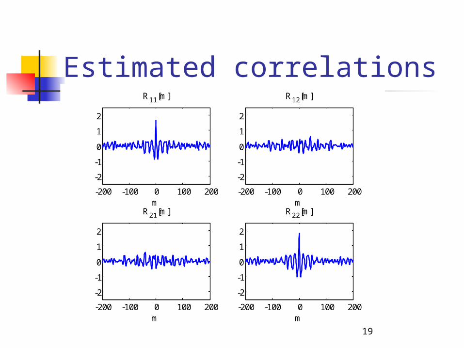
19

Estimated correlations

-200 -100 0 100 200

-2

-1

0

1

2

R11[m]

m-200 -100 0 100 200

-2

-1

0

1

2

R12[m]

m

-200 -100 0 100 200

-2

-1

0

1

2

R21[m]

m-200 -100 0 100 200

-2

-1

0

1

2

R22[m]

m

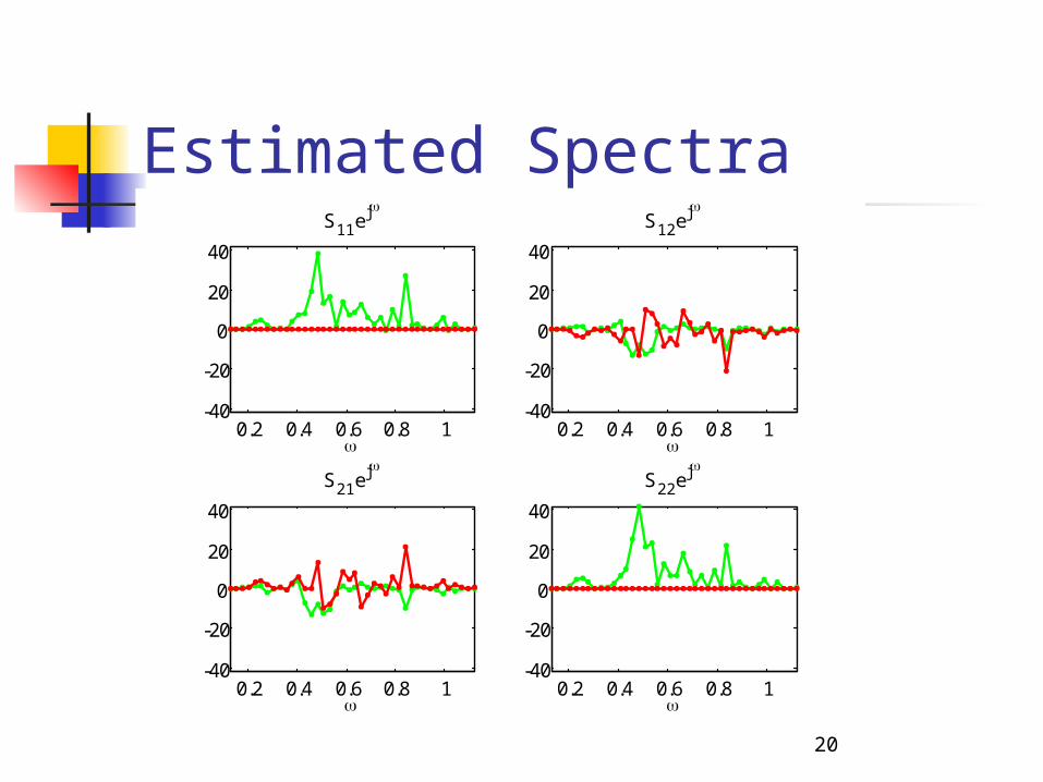
20

Estimated Spectra

0.2 0.4 0.6 0.8 1-40

-20

0

20

40

S11ej

0.2 0.4 0.6 0.8 1

-40

-20

0

20

40

S12ej

0.2 0.4 0.6 0.8 1-40

-20

0

20

40

S21ej

0.2 0.4 0.6 0.8 1

-40

-20

0

20

40

S22ej

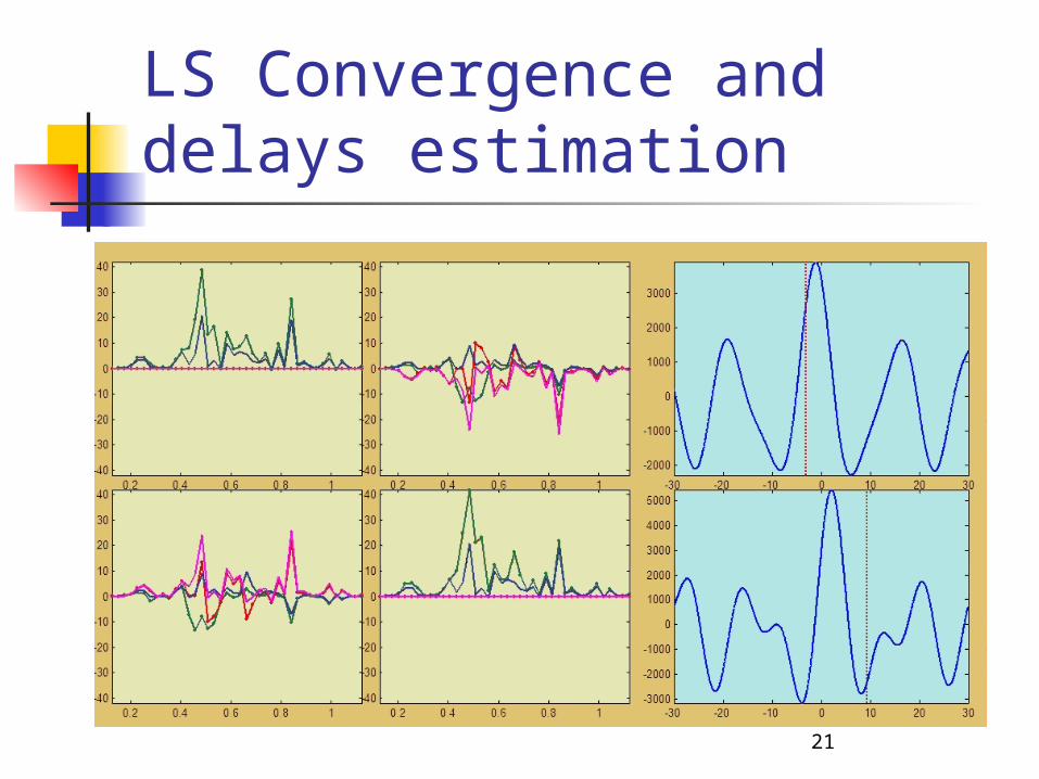
21

LS Convergence and delays estimation

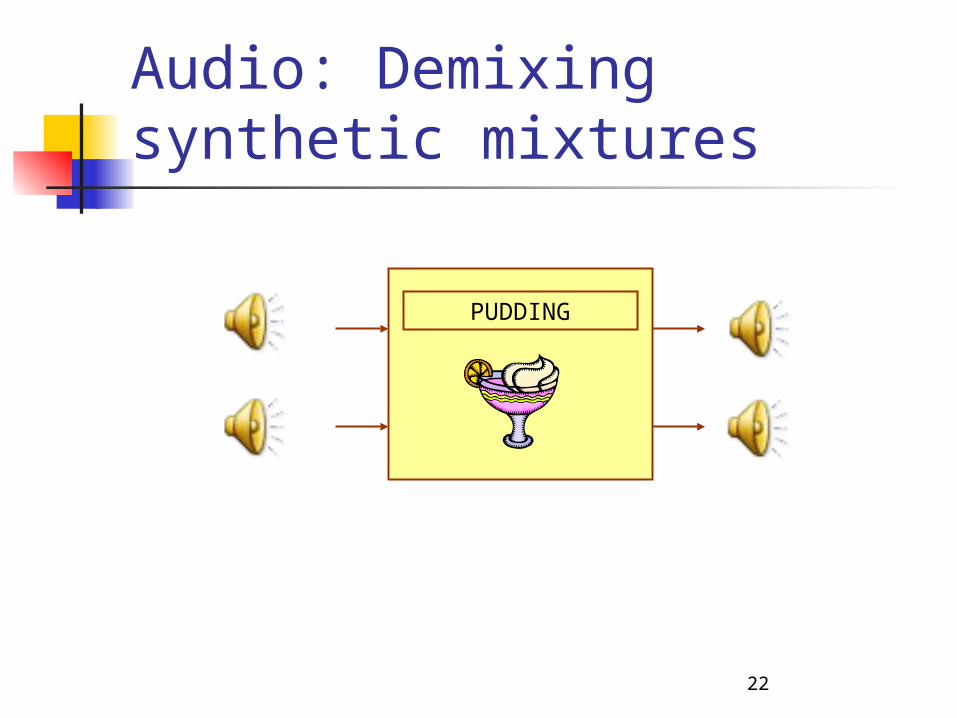
22

Audio: Demixing synthetic mixtures

PUDDING

23

Audio: “Demixing” synthetic mixtures ignoring delays

SEMI-GEENIE

We demonstrate the importance of estimating the delays, by demonstrating separation when the static mixing coefficients are known and the delays are ignored.

24

Audio: Robustness to additive white noise (3dB SNR)

PUDDING

25

True recordings: anechoic chamber setup (not to scale)

35cm

3m

2m600

PUDDING

Compare to [1]

26

Conclusions PUDDING – PUre Delays DemixING:

An iterative algorithm for BSS of anechoic mixtures involving unknown delays;

Works by optimizing a frequency-dependent joint diagonalization criterion;

Based on the extension of a static joint diagonalization algorithm (AC-DC), iterates between minimization w.r.t. the unknown spectra, coefficients and delays;

Typical convergence – within 10-20 iterations; Although the derivation assumed stationarity for simplicity,

the only essential assumption is persistent decorrelation between sources – good performance with speech sources.

Some frequency-dependent regularization is required when the static mixing coefficients form a nearly-singular matrix (not discussed here, due to timing constraints).