1-1

CMPE 259 Sensor Networks

Katia Obraczka

Winter 2005

Routing Protocols II

1-2

Announcements

Reading assignment 1 is up.

1-3

Notes on Directed Diffusion

Multiple paths can be used to forward data back to the sink.

Is it the same as multicast?

1-4

Data MULEs

1-5

Target deployments.

Sparse networks. Multi-tiered deployments.

Sensors. Wired access points. Mules.

1-6

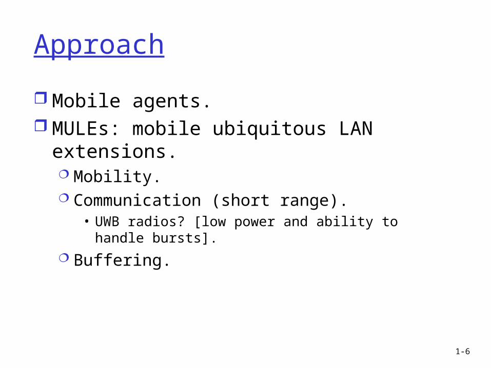
Approach

Mobile agents. MULEs: mobile ubiquitous LAN

extensions. Mobility. Communication (short range).

• UWB radios? [low power and ability to handle bursts].

Buffering.

1-7

Pros and cons

1-8

Pros and cons

Pros: Energy efficiency ?

• Listen for the mule. Intermittent connectivity.

Cons: Increased latency.

1-9

Alternatives

Approaches Latency Power Reliability Infrastructure cost

Base stations Low High High High

Ad-hoc Medium M/L Medium M/H

MULE High Low Medium Low

1-10

3-tier architecture

Wired APs. Mules. Sensors.

1-11

Considerations

APs have no limitations. Mules:

Storage, mobility, ability to communicate with sensors and APs.

Unpredictable movement patterns. Can talk to other mules.

• Benefits?

Robustness. Reliability.

1-12

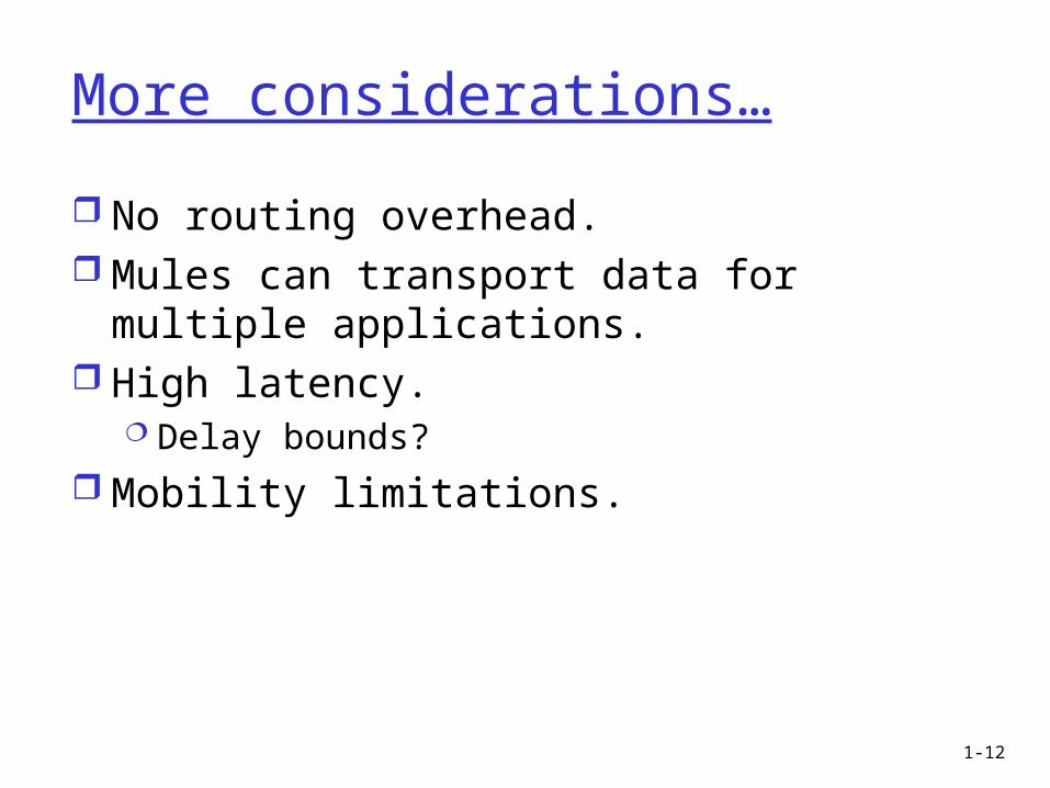
More considerations…

No routing overhead. Mules can transport data for multiple

applications. High latency.

Delay bounds? Mobility limitations.

1-13

System model

Simple, discrete. Lots of assumptions.

Realistic? Performance metrics:

Reliability. Buffer size. Delay?

1-14

Main results

Buffer requirements at sensors inversely proportional to ratio of number of mules to grid size.

Buffer requirement at mule inversely proportional to ratio of number of mules to grid size and ratio of APs to grid size.

Relationship between buffer capacity, number of mules, and reliability.

1-15

Energy-efficient routing

1-16

[Schurgers et al.]

Two approaches: Efficient data collection using aggregation. Load balancing: spread traffic uniformly.

1-17

Observations

Energy-optimal routing needs to consider future traffic. Energy limitations.

B

D

FA

C

E

T0 A and E send 50 pkts to B.

T1 F sends 100 pkts to B.

Load balancing: ADB, ECB, FDB.

But, if nodes can only send 100 pkts,D would no be able to deliver all ofF’s pkts to B.

In this case, ACB, ECB, FDB.

1-18

Energy-efficient versus energy-optimal Statistically optimal and only considers

causal information.

Lifetime:worst-case time until node fails.

1-19

Traffic spreading

Make sure that nodes are used uniformly by routing.

Gradient-based routing (GBR): Directed-diffusion variant. Use shortest path (in number of hops) to

sink to forward data.

Performance metric: ERMS. Root mean square of the PDF of energy

used by nodes.

1-20

Traffic spreading approaches

Stochastic: node picks next-hop randomly (chosen from neighbors with equal gradient).

Energy-based: node increases its “height” when its energy falls below a certain threshold. All nodes need to adjust their height accordingly.

Stream-based: divert streams from nodes that are part of paths used b other streams.

1-21

Results

Target tracking scenario. Stream-based spreading performs the

best. Stochastic spreading does better than

energy-based and pure GBR.

1-22

[Krishnamachari et al.]

1-23

Energy-robustness tradeoff in multipath routing Multipath for robustness.

Fault-tolerance through redundancy.

Alternatively, reduce number of intermediate nodes. Single paths. Nodes use higher transmit power.

1-24

Considerations Energy metric: number of transmissions

* transmit energy. Independent of number of receivers.

Robustness metric: Probability message reaches sink in the face

of node failures. Assume that nodes fail with probability p

independently from other nodes. Pareto optimality criteria:

Routing scheme dominates another iff more robust with strictly less energy, or

Iff it uses equal or less energy with strictly higher robustness.

1-25

Results

For the simple scenario chosen (with path loss exponent equal to 2), the Pareto optimal schemes only include single-path routing.

For higher path loss exponent, some multipath schemes are dominated by single path routing.