089 ' # '6& *#0 & 7cdn.intechopen.com/pdfs-wm/32912.pdf · san quintin lagoon...

3,350+OPEN ACCESS BOOKS

108,000+INTERNATIONAL

AUTHORS AND EDITORS115+ MILLION

DOWNLOADS

BOOKSDELIVERED TO

151 COUNTRIES

AUTHORS AMONG

TOP 1%MOST CITED SCIENTIST

12.2%AUTHORS AND EDITORS

FROM TOP 500 UNIVERSITIES

Selection of our books indexed in theBook Citation Index in Web of Science™

Core Collection (BKCI)

Chapter from the book Water Resources Management and ModelingDownloaded from: http://www.intechopen.com/books/water-resources-management-and-modeling

PUBLISHED BY

World's largest Science,Technology & Medicine

Open Access book publisher

Interested in publishing with IntechOpen?Contact us at [email protected]

http://www.intechopen.com/books/water-resources-management-and-modeling

mailto:[email protected]

6

San Quintin Lagoon Hydrodynamics Case Study

Oscar Delgado-González, Fernando Marván-Gargollo, Adán Mejía-Trejo and Eduardo Gil-Silva

Instituto de Investigaciones Oceanológicas, Universidad Autónoma de Baja California,

Ensenada, Baja California, México

1. Introduction

Hydrodynamics at coastal zone determine the way in which water flows and biochemical properties are exchanged. It is important to understand these processes in order to determine the potential effects caused by modifying the flow field as well as the mixing processes. For aquaculture purposes, the flow field distributes food to the organisms, thus by understanding the system hydrodynamic it is possible to determine suitable areas for aquaculture activities.

In México, approximately 2% of the 1.9 × 106 km2 which constitutes the national territory corresponds to protected or semi protected coastal areas (Ortiz-Pérez and Lanza-Espino 2006) and is distributed over 11,000 km of coastline; however, norms and guidelines for commercial aquaculture development were not established until the early 1990s, so this activity is currently at an incipient stage in most coastal areas.

San Quintin Lagoon (SQL) is a coastal lagoon located on the northwestern coast of Baja California (Mexico) which is characterized as a semiarid region with a highly productive upwelling offshore. The lagoon covers an area of approximately 42 km2 (Figure 1) and is divided in two basins named Bahia San Quintin (BSQ) and Bahia Falsa (BF). The mouth of the lagoon is 1 km wide and has maximum depth of 14 m. The lagoon shows several mud flats, some of them are exposed during low tides and others leave shallow areas which are optimal for aquaculture activities. The tidal regime is mixed semidiurnal with amplitudes as high as 1.6 m above MLLW (Mean Lower Low Water) during spring tides. The oceanic water entering the lagoon is nutrient rich due to upwelling processes associated with the north-south orientation of the coastline which mainly occur during spring and summer (Hernández-Ayón et al. 2004). The wind regime changes on a diurnal scale and is a breeze type with its maximum magnitude around 3pm with a dominant direction from the northwest. Due to the orientation of the lagoon and shallowness, the wind plays a very important role in circulation and generation of fetch limited waves. Inside the lagoon, the water column is well mixed (Millán-Núñez et al. 1982). The climate is Mediterranean and the lagoon shows as a negative estuary structure due to its net evaporation which makes the lagoon a hyper saline system throughout the year.

www.intechopen.com

Water Resources Management and Modeling 128

Fig. 1. Bahia San Quintin is a coastal lagoon on the northwest coast of Baja California México. The flags at the marine area represent the temperature sensor location, the one at the northwest continental location, marks the site location of the meteorological station.

During the 70s, studies were conducted at SQL to establish its viability for aquacultural activities (Lara-Lara and Álvarez-Borrego 1975, Álvarez-Borrego and Álvarez-Borrego 1982). These studies provided the first biophysical data and, among other findings, it was determined that the system is governed by mixed, semidiurnal tides.

In SQL, aquaculture activities have been conducted continuously for more than 30 years. The Pacific oyster Crassostrea gigas is extensively cultured in this area using a rack method. Even though most oyster farms use the same cultivation method, it is common to find differences of more than two months in the time at which organisms attain a commercial size throughout the lagoon (García-Esquivel et al. 2000).

The main factors involved in the selection of an area for aquaculture activities are: water, temperature, salinity, depth, and food availability (Héral and Deslous-Paoli, 1991). The conceptual model of factors and processes involved in the distribution of water properties by currents in BF (Delgado-González, 2010), gives an idea of the hydrodynamics and its importance in mixing and carrying food sources from one area to another. Phytoplankton spatial distribution at BF under neap and spring tides, considering oyster consumption, was obtained by using a 2D hydrodynamic model (Delgado-González, et al., 2010) and the results were utilized to determine the most productive areas within BF.

The purpose of this chapter is to present the hydrodynamic regimes at BSQ using a 2D hydrodynamic numerical model that considers the wind effect as well as analyzing food input to the lagoon, residence times and waste production within the lagoon by using a lagrangean tracker method. It is necessary to understand the possible circulation patterns of coastal lagoons like BSQ in order to adequately manage their resources and their water quality, which could be affected as a consequence of the aquaculture activities taking place inside the lagoon.

www.intechopen.com

San Quintin Lagoon Hydrodynamics Case Study 129

The hydrodynamics regimes and waterborne particle transport was obtained using the Coastal Modeling System Flow (CMS) Flow in conjunction with the Particle Tracking Model (PTM). Both models are embedded within the SMS user interface. CMS is a two-dimensional finite volume numerical model developed by the US Army Corps of Engineers which is based on a rectangular grid allowing for grid refinement as well as telescoping grids. PTM (Particle Tracking Model) is a lagrangean particle tracker designed to trace the fate and pathways of sediment and other waterborne particles. It was designed jointly by the Coastal Inlets Research Program (CIRP) and the Dredging Operations and Engineering Research (DOER). Particles are transported by the flow field and it takes into consideration a logarithmic current profile for their advection.

2. Data collection

2.1 Tides

Tides in the north Pacific coast are the primary hydrodynamic forcing agent for coastal lagoons with a constant water exchange with the open ocean such as SQL. (Fischer et al., 1979). The tides at SQL are mixed with a semidiurnal predominance (Figure 3). The tides exhibit a well-defined fortnightly modulation for which the range during spring tides is approximately 2.5 m and 1.0 m for neap tides. Using these values in combination with the surface area of the basin and the mouth cross-sectional area, for a linear-frictionless tidal wave, according to Stiegebrandt (1977), the amplitude of the tidal currents should be:

u0=ɑΥσ/2A

where α is the tidal range, Y is the surface area of the basin (42x106 m2), A is the cross-sectional area at the entrance (7500 m2) and σ is the frequency of the main tidal forcing (2π/12.42 h). Thus, for spring tides u0 should be approximately 0.98 m/s and for neap tides it should be around 0.31 m/s, which are similar to the observed values reported in this work.

The most intense tides occur during spring tides in December and January whilst the less exchange occurs during neap tides around the year (Delgado-Gonzalez, et al., 2010). There is a 40 minute tidal lag between the lagoon mouth and the head in BSQ, located in the inner part of the right arm of SQB (Ocampo-Torres 1980).

2.2 Wind

Wind, in many places, is responsible for producing surface currents as well as vertical mixing under special conditions (Fischer et al., 1979). In the particular case of San Quintin the wind is generally strong and the direction does not change very much thus being also an important forcing agent for the lagoon hydrodynamics. Due to the lagoon configuration, wind is more important at BF than at BSQ mainly due to the primary axis of BF which coincides with the predominant wind direction and the fact that volcanoes shelter BSQ.

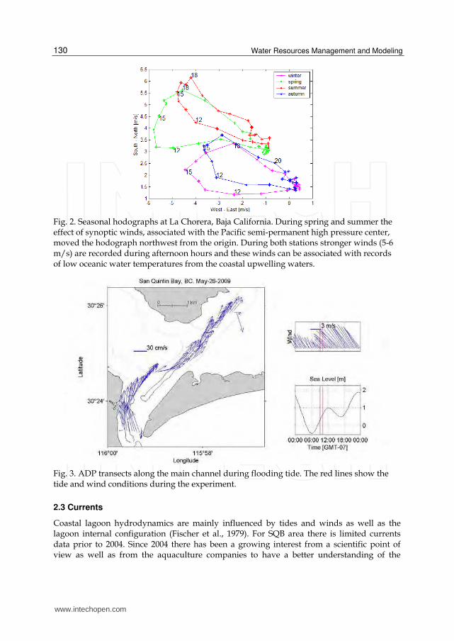
The wind data presented in this chapter was registered in the northwest area of BSQ (Figure 1). The wind hodograph shows the time of the day and magnitude for local and synoptic winds recorded at this station. This station also records air temperature and atmospheric pressure (Figure 2). The ellipse shape of the hodograph and its northern relative position from intersection of the West-East (u) and South-North (v) components can be used to identify the hourly characteristics for the local wind and the synoptic effect, respectively.

www.intechopen.com


Fig. 2. Seasonal hodographs at La Chorera, Baja California. During spring and summer the effect of synoptic winds, associated with the Pacific semi-permanent high pressure center, moved the hodograph northwest from the origin. During both stations stronger winds (5-6 m/s) are recorded during afternoon hours and these winds can be associated with records of low oceanic water temperatures from the coastal upwelling waters.

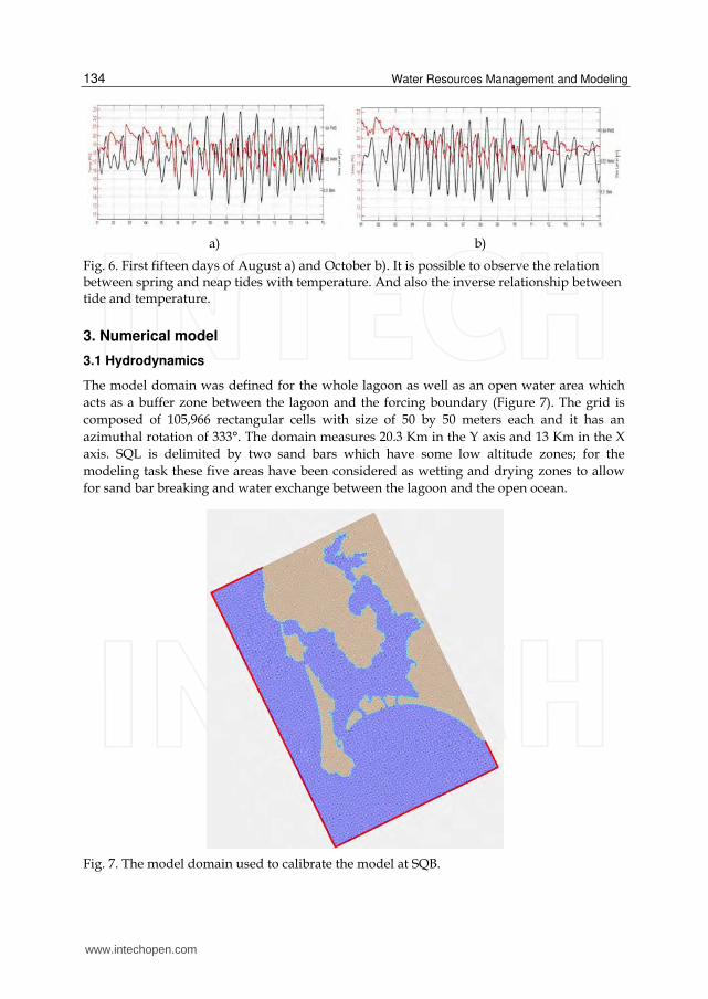
Fig. 3. ADP transects along the main channel during flooding tide. The red lines show the tide and wind conditions during the experiment.

2.3 Currents

Coastal lagoon hydrodynamics are mainly influenced by tides and winds as well as the lagoon internal configuration (Fischer et al., 1979). For SQB area there is limited currents data prior to 2004. Since 2004 there has been a growing interest from a scientific point of view as well as from the aquaculture companies to have a better understanding of the

www.intechopen.com


system circulation. To gain an idea of the hydrodynamics of San Quintin Lagoon, current data from ADP transects and drifters are shown next.

2.3.1 ADP transects

Several experiments were performed during different tidal and wind conditions. Figure 3 shows the depth averaged currents, flooding tide and wind conditions; it is possible to observe strong currents along the channels, a counter flow limited to the eastern part of the mouth and wind effects in the shallow areas. This experiment shows the complex circulation associated with the different forcing mechanisms; in some of them it is possible to recognize that the wind effect is mainly limited to the top layer (~1m).

2.3.2 Drifters

Field experiments using five drifters were done during 2010-2011 under ebb and flood tide conditions (Table 1).

Ebb tide

HWL to LWL Drifters

Time (h) Range (m) Date Initial time (To)

Ended time (Tf)

Distance (km)

Mean velocity (m s-1)

11:00-17:00 1.21 August 26, 2010

11:35 15:15 3.2 0.2

11:09-17:43 1.95 September 10, 2010

15:41 16:46 2.9 0.6

7:18-14:09 2.23 November 4, 2010

11:17 14:05 6.0 0.8

7:09-13:40 1.57 April 14, 2011

9:29 12:05 6.1 0.5

Flood tide

LWL to HWL

13:00-19:25 1.34 April 13, 2011

13:07 14:45 1.4 0.3

8:06-14:50 1.38 June 21, 2011

12:02 13:34 2.0 0.4

Table 1. The tidal condition during six field experiments with drifters at San Quintin Bay. During ebb tide the experiments conditions were from high water level (HWL) to low water level (LWL), and from LWL to HWL during flood tide.

For three of the experiments during ebb conditions, the drifters were located approximately 50 m apart from each other across the tidal channel; after being deployed, the ebb tide currents moved them to the central area of the tidal channel. In the August 26, 2010 experiment, the drifters were located approximately 100 m apart from each other along the central line of the tidal channel and their four hour trajectories remained along this central area.

www.intechopen.com


Drifters from September 10th, pink color (Figure 4a), were deployed at the central zone of BSQ. The five drifters finished out of the lagoon and most of the time their trajectories remained at the central part of the main tidal channel. Just at the mouth area, the drifters were closer to the east part rather than to the central part of the channel and ended at the shoaling region of the tidal delta. Drifters from November 4th, 2010 and April 14th, 2011, black and gold color (Figure 4a), followed the central area of the channel until they reached the delta part, where they started to move away from each other following curved trajectories, which indicates the balance between the lagoon water and the oceanic waters. Drifters from August 26th, 2010, red color (Figure 4a) located at the inner part of BSQ moved slower, but followed the central area of the tidal channel.

Drifters from April 13th, 2011, red color (Figure 4b) were located outside the bay in order to determine if they would be suctioned inside. However the wind component was strong enough to move them away from the bay entrance. On June 21st, 2011, black color (Figure 3b), the drifters were deployed 4 hours after the flooding tide started to fill the lagoon, reducing the possibility of seeing the full expected trajectories and the drifters were forced by the wind stress to curve into the sand bar.

a) b)

Fig. 4. During ebb tide conditions the mean velocities of drifters were 0.4m/s with maximum values around .8 m/s at the mouth area. During the experiments in flood conditions, the wind stress at the surface moved the drifters away when these were deployed outside San Quintin bay and to the coast when were deployed at the mouth. The initial time (To) is shown to represent the initial position in each experiment. The black arrow represents the outflow from and inflow to San Quintin Bay.

2.3.3 Water temperature

Water temperature at San Quintin Lagoon shows a clear seasonal signal, a clear variation between BF and BSQ and throughout a tidal cycle, and within its shallows areas the water temperature closely tracks air temperatures even with the constant effects of wind mixing processes.

www.intechopen.com


Three HOBO Water Temp Pro v2 Data Logger sensors were deployed at BSQ during the 6 months (Figure 1). These sensors were located at aquaculture buoys and situated at a depth of approximately 1.5 m. The instrument recorded temperature at a rate of 15 minutes (Figure 5). The role of tides in the temperature oscillations during the August-November months and the upwelling index is well observed; it is possible to observe that during spring tides the water temperature inside the lagoon drops 3 or 4 0C, and most of the times this drop shows visual correlation with the upwelling index, and during neap tides the system increase its temperature. However, during the last days of November the spring tides reduce the temperature and the system does not return to the original warm temperatures, marking the beginning of winter inside the lagoon (Figure 5).

Fig. 5. The temperature time series at three stations in BSQ showed similar behavior, only two are presented. During summer months mean temperatures in the two inner is 19.0 C ± 1.44 and 14.8 C± 0.95 during winter months. The fortnightly tide has an important role in the main fluctuations observed.

In order to see the relationship between spring and neap tides and temperature changes, the first fifteen days of August and October (Figure 6). During neap tides, first 6 days of August (Figure 6a) the mean temperature is around 19 o C and during the spring tide the mean temperature remains around 17.5 o C, mainly because of the different hydrodynamics associated with these two tide conditions.

www.intechopen.com


a) b)

Fig. 6. First fifteen days of August a) and October b). It is possible to observe the relation between spring and neap tides with temperature. And also the inverse relationship between tide and temperature.

3. Numerical model

3.1 Hydrodynamics

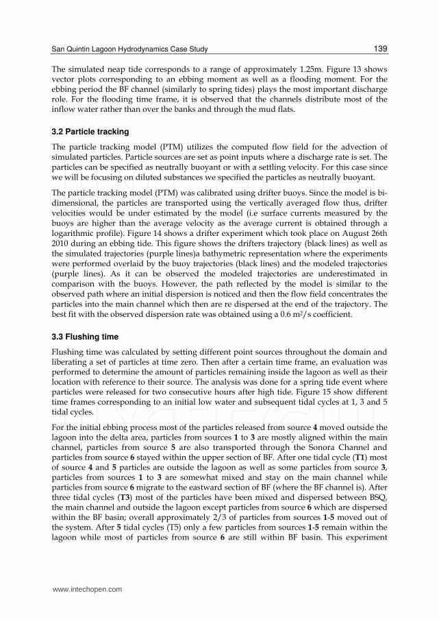
The model domain was defined for the whole lagoon as well as an open water area which acts as a buffer zone between the lagoon and the forcing boundary (Figure 7). The grid is composed of 105,966 rectangular cells with size of 50 by 50 meters each and it has an azimuthal rotation of 333°. The domain measures 20.3 Km in the Y axis and 13 Km in the X axis. SQL is delimited by two sand bars which have some low altitude zones; for the modeling task these five areas have been considered as wetting and drying zones to allow for sand bar breaking and water exchange between the lagoon and the open ocean.

Fig. 7. The model domain used to calibrate the model at SQB.

www.intechopen.com


The domain bathymetry was created using data reported by Flores (2006) and actualized with data collected 2009, 2010 and 2011 field work experiments; data set is referenced to mean low water. The resulting depths (Figure 8) clearly show the main channel as well as the bifurcation between BSQ and BF. The estuary delta is observed mainly at the east side of the estuary mouth. but a fan-shaped submerged sand bar is also visible surrounding the mouth. Inside the lagoon the orange colors represent the mud flat areas and it can be observed that the majority of the lagoon is shallow (between 0.5m and 1.5m).

Fig. 8. Model bathymetry and calibration point A.

The main forcing processes within the lagoon are tide, most important, and wind (of secondary importance). At the open boundary (shown in Figure 7 as a red line) water surface elevation fluctuations due to tides are specified and all over the domain surface spatially constant wind condition is specified. To calibrate the model, wind and water surface elevation (WSE) data corresponding to a spring tide event from May 30, 2004 through June 10, 2004 was used (Figure 9). At the same time, Acoustic Doppler Profile (ADP) data from a fixed location (point A at Figure 8) was used to compare against model results. The comparison between observed and modeled current magnitude at point A (Figure 10), shows that a close relationship can be seen except at high magnitude currents where the model underestimates the currents by approximately 0.01m/s. Figure 11 shows a correlation plot between modeled and observed current magnitude and a R2 factor of 0.87 was obtained.

Fig. 9. Observed tidal period from May 30 to June 10, 2004.

-1.5

-1

-0.5

0

0.5

1

1.5

5/29 5/30 5/31 6/1 6/2 6/3 6/4 6/5 6/6 6/7 6/8 6/9 6/10 6/11

WS

E (

m)

Time (days)

Tidal variation

www.intechopen.com


Fig. 10. Observed (red line) and simulated (blue line) current magnitude.

Fig. 11. Correlation between observed and simulated currents

Simulation results corresponding to spring and neap tide periods are presented in this section. The spring tide cycle corresponds to September 6th and 7th 2010 where the tidal range at the mouth was 2.25m. Figure 12 shows vector plots corresponding to ebbing and flooding moments for this particular tidal cycle. As the tide starts to descend, the flow field from the shallow areas converge at the main channels. At this point the most significant flow contribution to the main discharge originates from the west side of BF which is abundant in aquaculture activities. After approximately 1.5 hours, the flow field is well established at the BSQ Channel and Sonora Channel but is less evident at BF Channel. After four hours the strongest flow is mainly around the channels while the mud flats contribution is less significant. Finally after five hours the flow field is mostly observed at the channels. Throughout the ebbing period BSQ channel shows the most discharge. At the estuarine mouth, the flow follows the main channel and then forms a fan shaped flow field with the strongest currents observed at the southern section of the estuary entrance. As the tide changes, water starts to propagate inwards mainly through the southern section of the mouth in a funnel shape. Inside the lagoon the flow propagates mainly through the channels. For BF both channels contribute equally with the flow field propagating into the mud flats and a convergence of both water masses can be observed in the central area of this mud flat. After approximately 2.5 hours from low tide the water starts to propagate over the mud flat between Sonora Channel and BF Channel as well as over the east bank of the BSQ Channel. This pattern is then observed until the flooding process ends.

0.0

0.2

0.4

0.6

0.8

1.0

1.2

5/29 5/30 5/31 6/1 6/2 6/3 6/4 6/5 6/6 6/7 6/8 6/9 6/10 6/11

Cu

rre

nts

(m

/s)

Time (days)

Ovserved vs measured currents

Simulated

Measured

y = 0.98x

R² = 0.8748

0.0

0.2

0.4

0.6

0.8

1.0

1.2

0.0 0.2 0.4 0.6 0.8 1.0 1.2 1.4

Sim

ula

ted

re

sult

s (

m/s

)

Observed data (m/s)

Observed vs simulated currents

www.intechopen.com


Fig. 12. (Top) Ebbing tide for a spring event, 3.5 hours after high water and (Bottom) flooding tide for a spring event, after 2.5 hours from low water.

www.intechopen.com


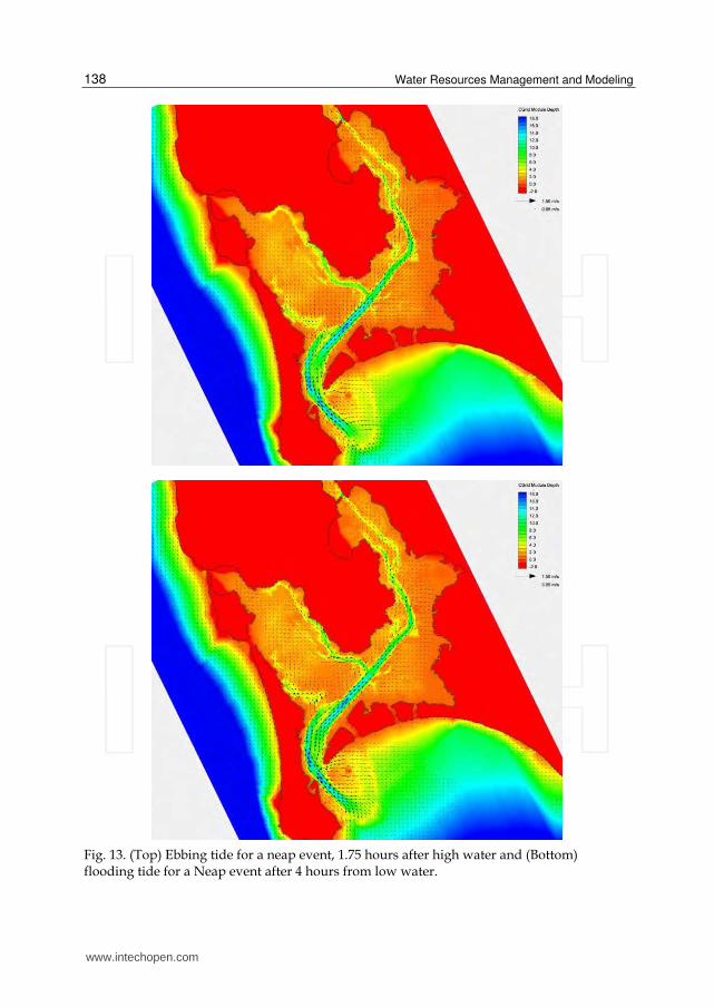
Fig. 13. (Top) Ebbing tide for a neap event, 1.75 hours after high water and (Bottom) flooding tide for a Neap event after 4 hours from low water.

www.intechopen.com


The simulated neap tide corresponds to a range of approximately 1.25m. Figure 13 shows vector plots corresponding to an ebbing moment as well as a flooding moment. For the ebbing period the BF channel (similarly to spring tides) plays the most important discharge role. For the flooding time frame, it is observed that the channels distribute most of the inflow water rather than over the banks and through the mud flats.

3.2 Particle tracking

The particle tracking model (PTM) utilizes the computed flow field for the advection of simulated particles. Particle sources are set as point inputs where a discharge rate is set. The particles can be specified as neutrally buoyant or with a settling velocity. For this case since we will be focusing on diluted substances we specified the particles as neutrally buoyant.

The particle tracking model (PTM) was calibrated using drifter buoys. Since the model is bi-dimensional, the particles are transported using the vertically averaged flow thus, drifter velocities would be under estimated by the model (i.e surface currents measured by the buoys are higher than the average velocity as the average current is obtained through a logarithmic profile). Figure 14 shows a drifter experiment which took place on August 26th 2010 during an ebbing tide. This figure shows the drifters trajectory (black lines) as well as the simulated trajectories (purple lines)a bathymetric representation where the experiments were performed overlaid by the buoy trajectories (black lines) and the modeled trajectories (purple lines). As it can be observed the modeled trajectories are underestimated in comparison with the buoys. However, the path reflected by the model is similar to the observed path where an initial dispersion is noticed and then the flow field concentrates the particles into the main channel which then are re dispersed at the end of the trajectory. The best fit with the observed dispersion rate was obtained using a 0.6 m2/s coefficient.

3.3 Flushing time

Flushing time was calculated by setting different point sources throughout the domain and liberating a set of particles at time zero. Then after a certain time frame, an evaluation was performed to determine the amount of particles remaining inside the lagoon as well as their location with reference to their source. The analysis was done for a spring tide event where particles were released for two consecutive hours after high tide. Figure 15 show different time frames corresponding to an initial low water and subsequent tidal cycles at 1, 3 and 5 tidal cycles.

For the initial ebbing process most of the particles released from source 4 moved outside the lagoon into the delta area, particles from sources 1 to 3 are mostly aligned within the main channel, particles from source 5 are also transported through the Sonora Channel and particles from source 6 stayed within the upper section of BF. After one tidal cycle (T1) most of source 4 and 5 particles are outside the lagoon as well as some particles from source 3, particles from sources 1 to 3 are somewhat mixed and stay on the main channel while particles from source 6 migrate to the eastward section of BF (where the BF channel is). After three tidal cycles (T3) most of the particles have been mixed and dispersed between BSQ, the main channel and outside the lagoon except particles from source 6 which are dispersed within the BF basin; overall approximately 2/3 of particles from sources 1-5 moved out of the system. After 5 tidal cycles (T5) only a few particles from sources 1-5 remain within the lagoon while most of particles from source 6 are still within BF basin. This experiment

www.intechopen.com


Fig. 14. Particle and buoy trajectories for August 26th ebbing tide.

www.intechopen.com


Fig. 15. Residence time for different zones within San Quintin Lagoon

www.intechopen.com


shows that the flushing time from BSQ is much faster than for BF, especially the upper section of this basin. Also the Sonora Channel plays an important role in flushing BF as can be observed from source 5 and the main channel connecting to BSQ flushes the eastern mud flats represented by sources 2 and 3.

3.4 Detritus inflow

Due to the fact that aquaculture is a very important activity inside BF basin, the model was set to simulate detritus inflow from open water into the lagoon. To do so, four point sources were specified just beyond the mouth delta. Figure 16 shows these sources as well as the advection of such particles during a flooding time frame.

From Figure 16a it can be observed that sources 1 and 2 are mainly transported into BF through the Sonora Channel, at the left side of BF, as well as over the central mud flat and a smaller fraction from this sources goes into SQB. For source 3 there is not much transported into the lagoon as the bulk stays outside and finally source 4 is transported through the main channel mostly into BSQ as well as the eastern mudflats from BSQ basin and just a very small fraction enters into BF basin.

Fig. 16. a) Modeled detritus inflow point sources and b) chlorophyll levels during a flooding period.

www.intechopen.com


Figure 16b shows chlorophyll data taken with a Turner design fluorometer in June 21st 2011 during a flooding time period. This plot shows higher concentrations on the western side of the mouth thus, this chlorophyll rich water will be introduced into BF basin and utilized by the cultivated oysters.

Another relevant finding from this experiment is that the upper sections of BF basin and SQB basin do not show many particles which suggests low quality water which for BF basin is asseverated as the flushing of residues produced on this area is also poor.

4. Acknowledgements

This work is a contribution of project by UABC grants 14avaConvocatoria Interna and by F-PROMEP-36 SEP-23-006 grants.

5. References

Alvarez-Borrego, J. y Alvarez-Borrego S. 1982. Temporal and spatial variability of temperature in two coastal lagoons. CalCOFI Reports XXIII:, 188-197.

Delgado-González, O.E. 2010. Desarrollo y aplicación de una herramienta de gestiónpara el aprovechamiento acuícola en Bahía San Quintín,Baja California. PhD Thesis. Universidad Politénica de Cataluña, Barcelona, España. 182 p.

Delgado-González, O.E., Jiménez, J.A., Fermán-Almada, J.L., Marván-Gargollo, F. , Mejía-Trejo, A. ,García-Esquivel, Z. 2010. La profundidad e hidrodinámica como herramientas para la selección de espacios acuícolas en la zona costera. Ciencias Marinas 36(3). 249-265.

Fischer, H.B. List, E.J., Koh, R.C.Y., Imberger, J. and Brooks, N.H. 1979. Mixing in inland and coastal waters. Academic Press, Boston, 483 pp.

Flores-Vidal, Xavier, 2006. Circulación Residual en Bahía San Quintín, B.C., México. CICESE. MSc. 91pp.

García-Esquivel, Z., González-Gómez M. A., Ley-Lou F. y Mejía-Trejo A. 2000. Microgeographic differences in growth, mortality, and biochemical composition of cultures pacific oysters (Crassostrea gigas) from San Quintin Bay, Mexico. Journal of Shellfish Research 19 2. 789-797.

Héral, M. y Deslous-Paoli J.M. 1991. Oyster culture in european countries. CRC Press, Inc. 154-186.

Hernández-Ayón, M, Galindo-Bect M.S., Camacho-Ibar V.F., García-Esquivel Z., González-Gómez M.A. y Ley-Lou F. 2004. Dinámica de los nutrientes en el brazo oeste de la Bahía de San Quintín, Baja California, México, durante y después de El Niño 1997/1998. Ciencias Marinas 30 1A. 129-142.

Lara-Lara, J.R. y Álvarez-Borrego S. 1975. Ciclo anual de clorofilas y producción orgánica primara en Bahía San Quintín, Baja California. Ciencias Marinas 2 1. 77-97.

Millán-Núñez, R., Alvarez-Borrego S. y Nelson D.M. 1982. Effects of physical phenomena on the distribution of nutrients and phytoplankton productivity in a coastal lagoon. Estuarine, Coastal and Shelf Science 15. 317-335.

www.intechopen.com


Ortiz-Pérez, M.A. and D.L. Lanza-Espino, 2006. Diferenciación del espacio costero de México: Un

inventario regional. México: Serie deTextos Universitarios, Instituto de Geografía-UNAM, México.137p.

Ocampo-Torres, F.J. 1980. Análisis y predicción de velocidad mediante un modelo unidimesional en Bahía San Quintín, B.C, México. Universidad Autónoma de Baja California BSc 90 pp.

Stigebrandt, A. 1977. On the effect of barotropic current fluctuations on the two-layer transport capacity of a constriction. Journal of Physical Oceanography 7, 118-122.

www.intechopen.com

Water Resources Management and ModelingEdited by Dr. Purna Nayak

ISBN 978-953-51-0246-5Hard cover, 310 pagesPublisher InTechPublished online 21, March, 2012Published in print edition March, 2012

InTech EuropeUniversity Campus STeP Ri Slavka Krautzeka 83/A 51000 Rijeka, Croatia Phone: +385 (51) 770 447 Fax: +385 (51) 686 166www.intechopen.com

InTech ChinaUnit 405, Office Block, Hotel Equatorial Shanghai No.65, Yan An Road (West), Shanghai, 200040, China

Phone: +86-21-62489820 Fax: +86-21-62489821

Hydrology is the science that deals with the processes governing the depletion and replenishment of waterresources of the earth's land areas. The purpose of this book is to put together recent developments onhydrology and water resources engineering. First section covers surface water modeling and second sectiondeals with groundwater modeling. The aim of this book is to focus attention on the management of surfacewater and groundwater resources. Meeting the challenges and the impact of climate change on waterresources is also discussed in the book. Most chapters give insights into the interpretation of field information,development of models, the use of computational models based on analytical and numerical techniques,assessment of model performance and the use of these models for predictive purposes. It is written for thepracticing professionals and students, mathematical modelers, hydrogeologists and water resourcesspecialists.

How to referenceIn order to correctly reference this scholarly work, feel free to copy and paste the following:

Oscar Delgado-González, Fernando Marván-Gargollo, Adán Mejía-Trejo and Eduardo Gil-Silva (2012). SanQuintin Lagoon Hydrodynamics Case Study, Water Resources Management and Modeling, Dr. Purna Nayak(Ed.), ISBN: 978-953-51-0246-5, InTech, Available from: http://www.intechopen.com/books/water-resources-management-and-modeling/san-quintin-lagoon-hidrodynamics-case-study

089 ' # '6& *#0 & 7cdn.intechopen.com/pdfs-wm/32912.pdf · san quintin lagoon...

Documents