EEE 309 Communication TheorySemester: January 2016Semester: January 2016

D Md F h d H iDr. Md. Farhad HossainAssociate Professor

Department of EEE, BUET

Email: mfarhadhossain@eee.buet.ac.bdOffice: ECE 331, ECE Building

Part 04

Angle ModulationAngle Modulation

2

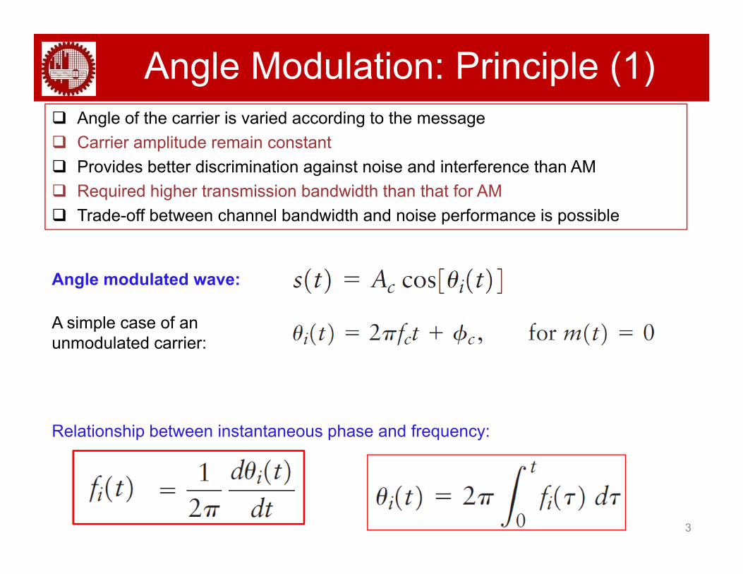
Angle Modulation: Principle (1) Angle of the carrier is varied according to the message Carrier amplitude remain constant Provides better discrimination against noise and interference than AM Required higher transmission bandwidth than that for AM Trade-off between channel bandwidth and noise performance is possible

Angle modulated wave:

A simple case of anA simple case of an unmodulated carrier:

Relationship between instantaneous phase and frequency:

3

Angle Modulation: Principle (2) Two common methods for angle modulation:

1. Phase Modulation (PM): kp = Phase sensitivity factor (radians/volt)

Phase-modulated signal:

2. Frequency Modulation (FM):kf = Frequency sensitivity factor (Hz/volt)

Frequency-modulated signal:

4

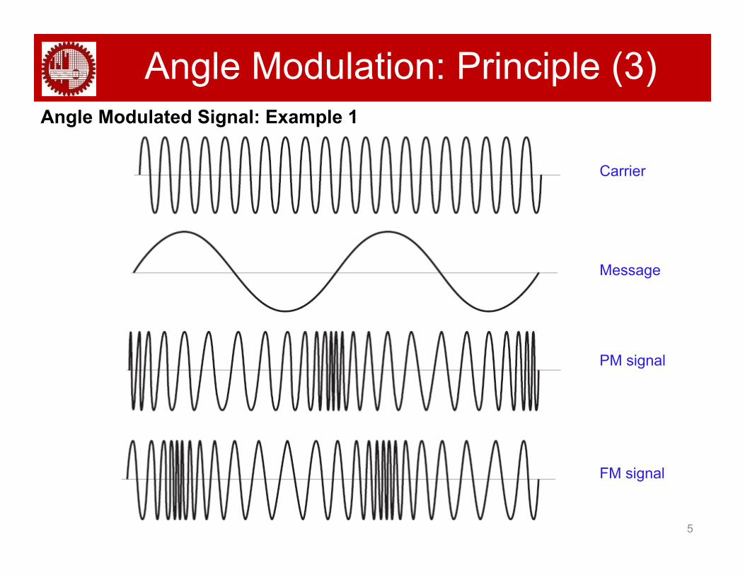
Angle Modulation: Principle (3) Angle Modulated Signal: Example 1

Carrier

Message

PM signal

FM i l

5

FM signal

Angle Modulation: Principle (4) Angle Modulated Signal: Example 2

Message

PM signalPM signal

FM signal

6

FM signal

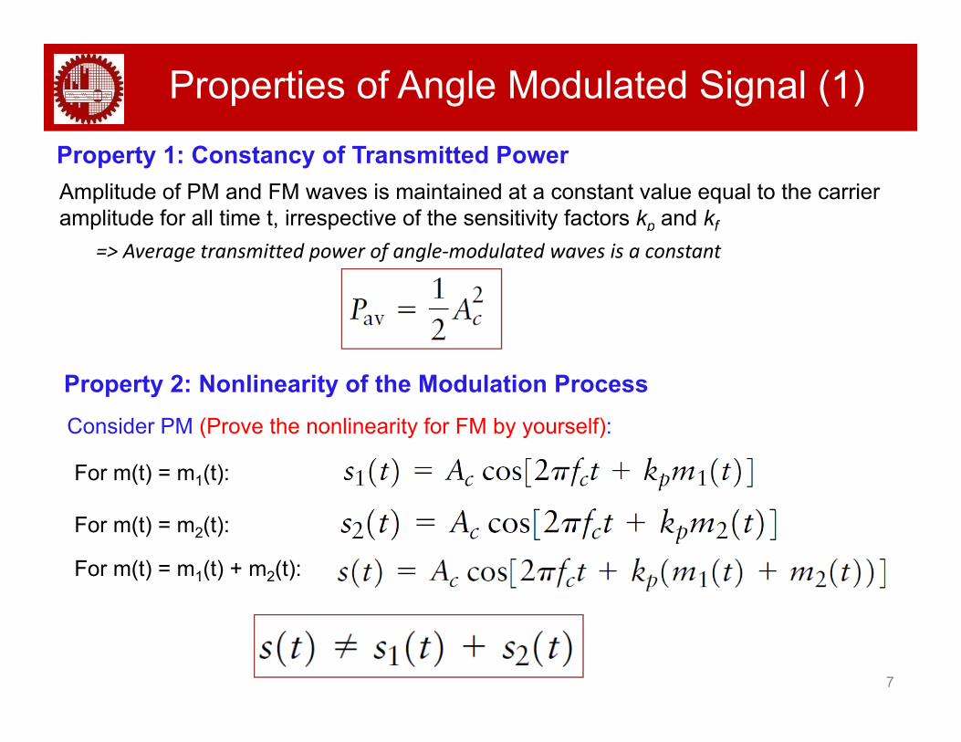
Properties of Angle Modulated Signal (1) Property 1: Constancy of Transmitted PowerAmplitude of PM and FM waves is maintained at a constant value equal to the carrier amplitude for all time t, irrespective of the sensitivity factors kp and kf

=> Average transmitted power of angle‐modulated waves is a constant

Property 2: Nonlinearity of the Modulation ProcessC id PM (P h li i f FM b lf)

For m(t) = m1(t):

Consider PM (Prove the nonlinearity for FM by yourself):

For m(t) = m2(t):

For m(t) = m1(t) + m2(t):

7

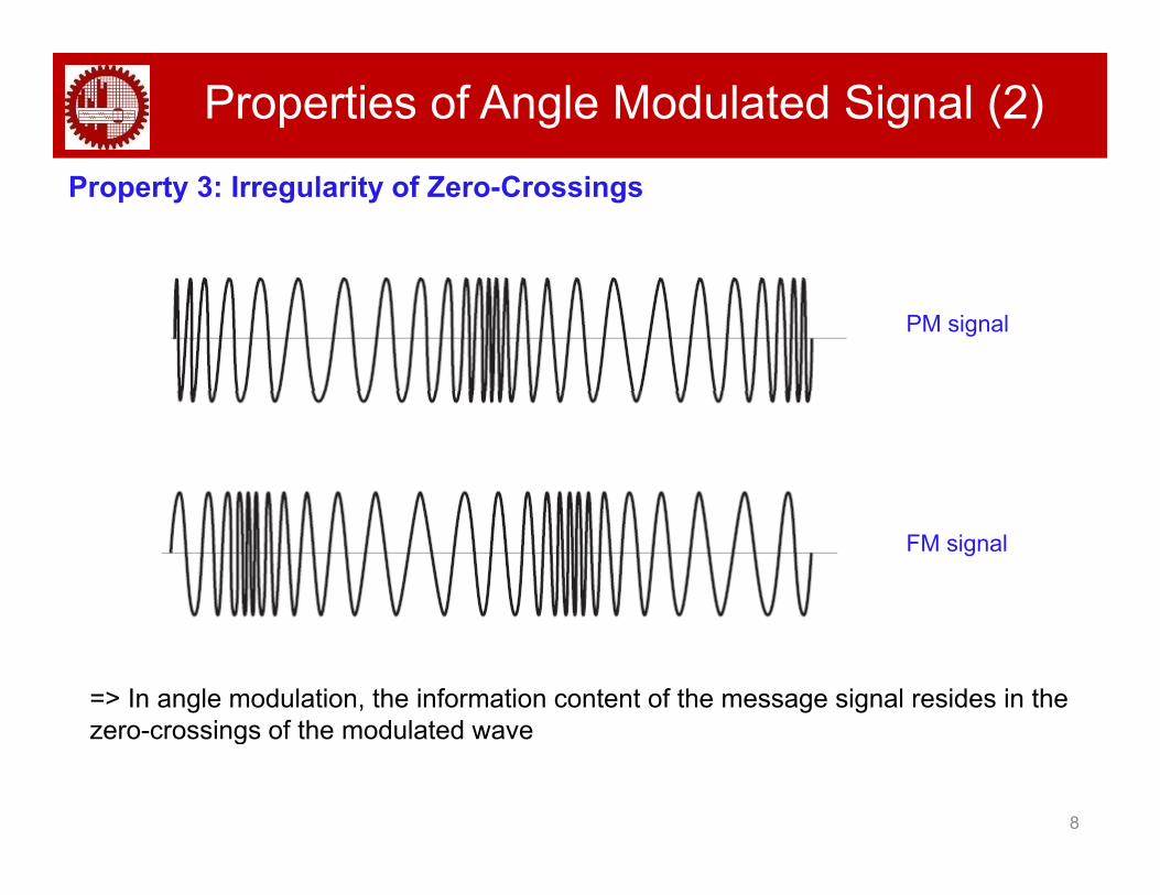
Properties of Angle Modulated Signal (2) Property 3: Irregularity of Zero-Crossings

PM signal

FM signal

=> In angle modulation, the information content of the message signal resides in the zero crossings of the modulated wave

8

zero-crossings of the modulated wave

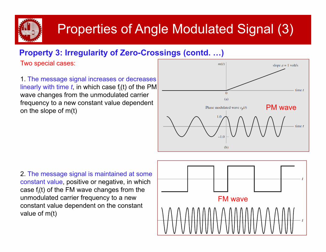
Properties of Angle Modulated Signal (3) Property 3: Irregularity of Zero-Crossings (contd. …)Two special cases:

1 The message signal increases or decreases1. The message signal increases or decreases linearly with time t, in which case fi(t) of the PM wave changes from the unmodulated carrier frequency to a new constant value dependent on the slope of m(t) PM wave on the slope of m(t)

2 The message signal is maintained at some2. The message signal is maintained at some constant value, positive or negative, in which case fi(t) of the FM wave changes from the unmodulated carrier frequency to a new constant value dependent on the constant

FM wave

9

constant value dependent on the constant value of m(t)

Properties of Angle Modulated Signal (4) Property 4: Visualization Difficulty of Message SignalThe difficulty in visualizing the message waveform in angle-modulated waves is attributed to the nonlinear character of angle-modulated waves

AMAM wave Easy to visualize the effect

PM wave Difficult to visualize

10

Properties of Angle Modulated Signal (5)

Property 5: Tradeoff of Increased Transmission Bandwidth for Improved Noise Performance An important advantage of angle modulation over AM is the realization of improved p g g pnoise performance

This advantage is due to the fact that the transmission of a message signal by modulating the angle of a sinusoidal carrier wave is less sensitive to the presence ofmodulating the angle of a sinusoidal carrier wave is less sensitive to the presence of additive noise than transmission by modulating the amplitude of the carrier

The improvement in noise performance is, however, attained at the expense of a corresponding increase in the transmission bandwidth requirement of angle modulation

In other words the use of angle modulation offers the possibility of exchanging an In other words, the use of angle modulation offers the possibility of exchanging an increase in transmission bandwidth for an improvement in noise performance.

Such a tradeoff is not possible with amplitude modulation since the transmission

11

bandwidth of an amplitude-modulated wave is fixed somewhere between the message bandwidth B and 2B Hz, depending on the type of modulation employed

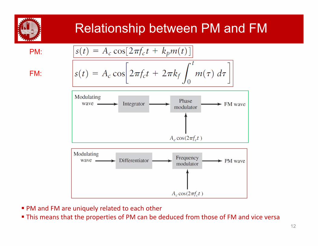
Relationship between PM and FM

FM:

PM:

12

PM and FM are uniquely related to each other This means that the properties of PM can be deduced from those of FM and vice versa

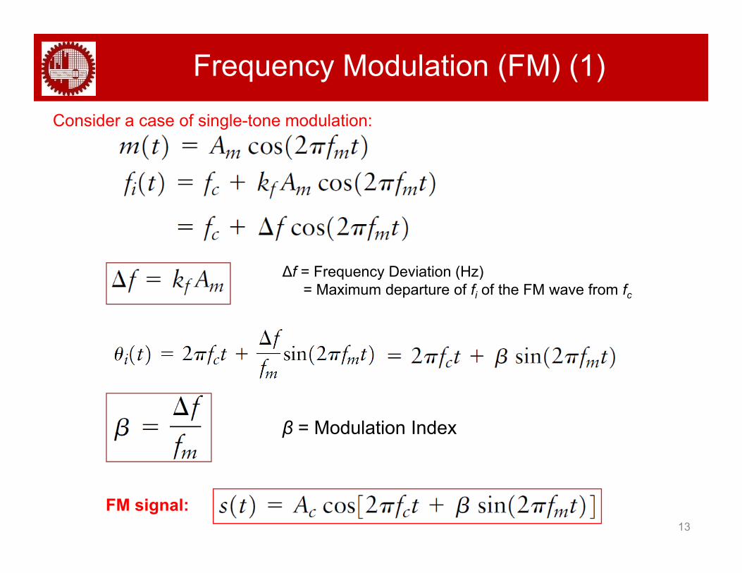
Frequency Modulation (FM) (1)Consider a case of single-tone modulation:

Δf = Frequency Deviation (Hz) = Maximum departure of fi of the FM wave from fc

β = Modulation Index

13

FM signal:

Narrow-band FM (NBFM) 1. NBFM (β is small compared to one radian):

For small β:

14

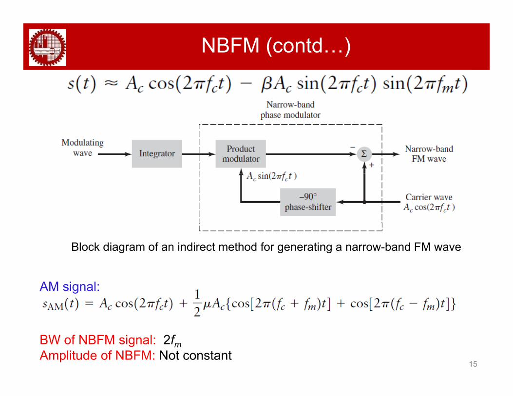
NBFM (contd…)

Block diagram of an indirect method for generating a narrow-band FM wave

AM signal:

15

BW of NBFM signal: 2fmAmplitude of NBFM: Not constant

Wide-band FM (WBFM) 2. WBFM (β is large compared to one radian):

Complex Envelope of s(t):Complex Envelope of s(t):

=> a periodic function of time with a fundamental frequency equal to fm a periodic function of time with a fundamental frequency equal to fm

16

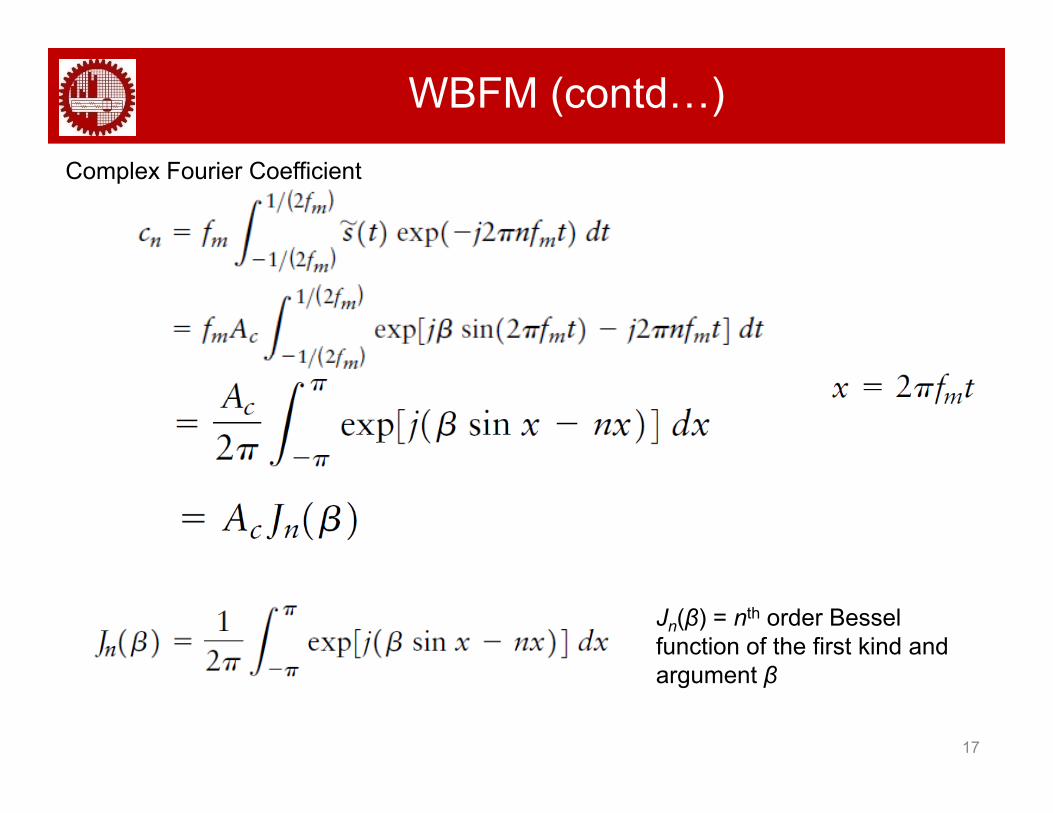
WBFM (contd…)Complex Fourier Coefficient

Jn(β) = nth order Bessel function of the first kind and

17

argument β

WBFM (contd…)Thus,

=> S(f) consists of an infinite number of delta functions spaced at f = fc ± nfm

18

WBFM (contd…)Properties of FM for arbitrary β:

1. Jn(β) = (-1)n J-n(β) for all n

3.

19

WBFM (contd…)1. The spectrum of an FM wave contains a carrier component and an infinite set of

side frequencies located symmetrically on either side of the carrier at frequency separations of fm, 2fm, 3fm, ….

2. For the special case of small β compared with unity, only the Bessel coefficients J0(β) and J1(β) have significant values, so that the FM wave is effectively composed of a carrier and a single pair of side-frequencies at fc±fm. This FM p g p q c msignal is essentially the NBFM signal.

3. The amplitude of the carrier component varies with β according to J0(β). This implies that the envelope of an FM wave is constant so that the average powerimplies that the envelope of an FM wave is constant, so that the average power of FM signal is constant.

Power of FM signal

20

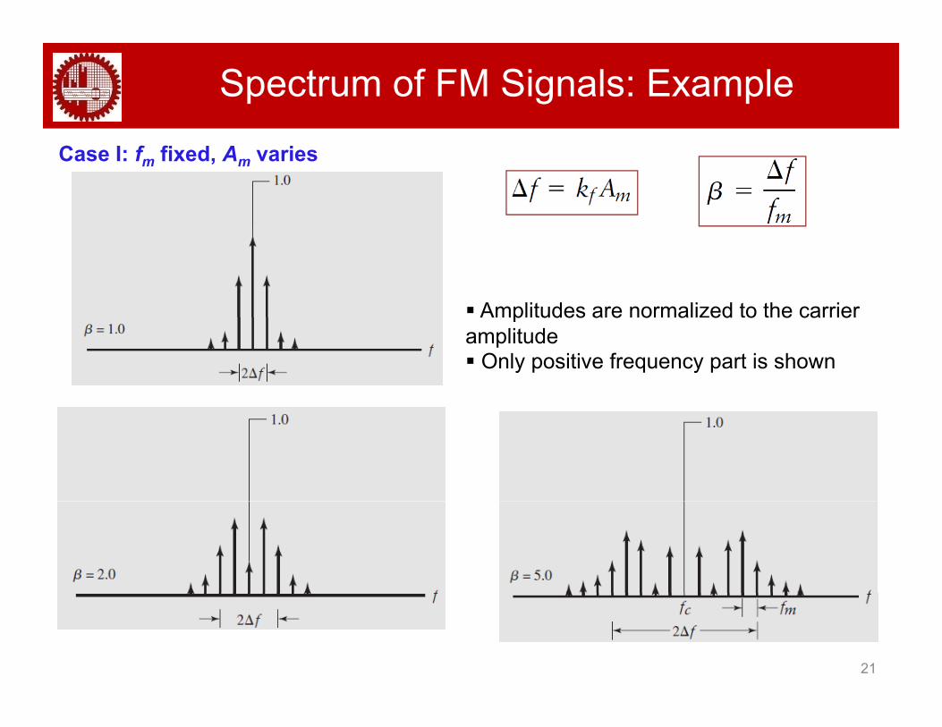
Spectrum of FM Signals: ExampleCase I: fm fixed, Am varies

Amplitudes are normalized to the carrier p udes a e o a ed o e ca eamplitude Only positive frequency part is shown

21

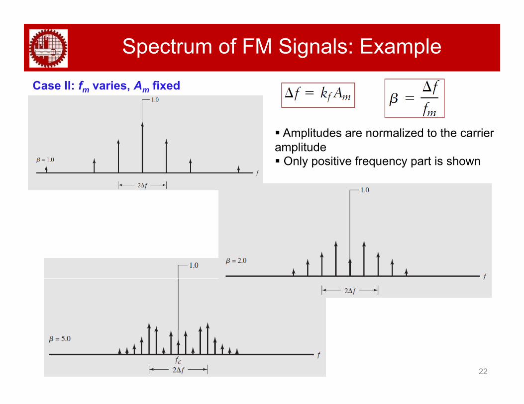
Spectrum of FM Signals: ExampleCase II: fm varies, Am fixed

Amplitudes are normalized to the carrier amplitude Only positive frequency part is shown

22

BW of FM Signals

Method 1: Carson’s Rule

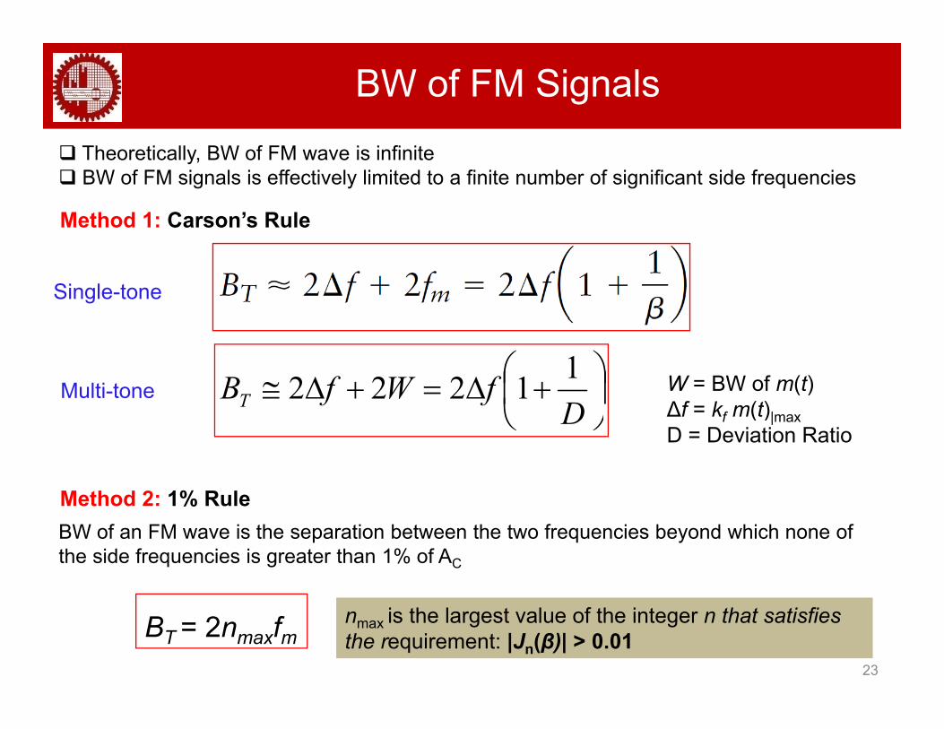
Theoretically, BW of FM wave is infinite BW of FM signals is effectively limited to a finite number of significant side frequencies

Method 1: Carson s Rule

Single-tone

DfWfBT

11222 W = BW of m(t)Δf = k m(t)

Multi-tone D Δf = kf m(t)|max

D = Deviation Ratio

Method 2: 1% RuleMethod 2: 1% RuleBW of an FM wave is the separation between the two frequencies beyond which none of the side frequencies is greater than 1% of AC

23

BT = 2nmaxfmnmax is the largest value of the integer n that satisfies the requirement: |Jn(β)| > 0.01

BW of FM Signals

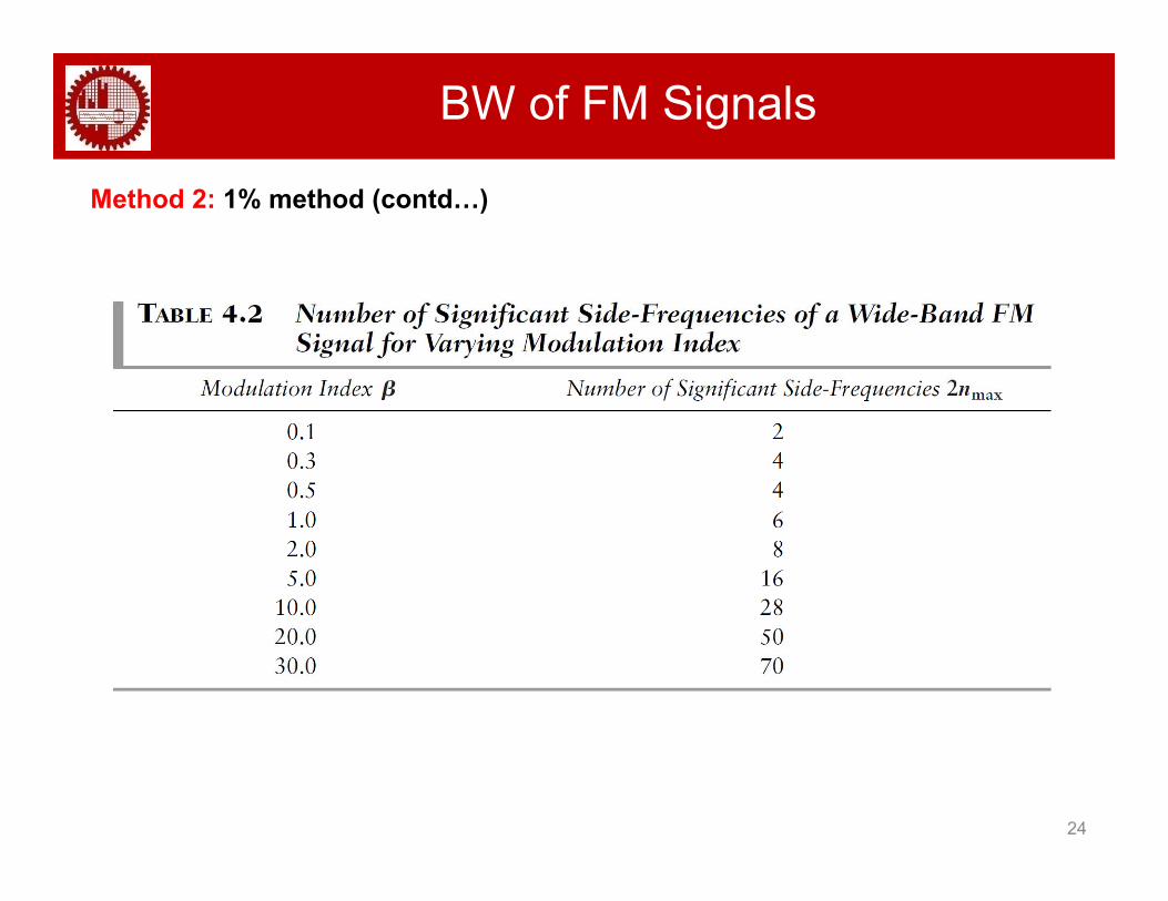
Method 2: 1% method (contd…)

24

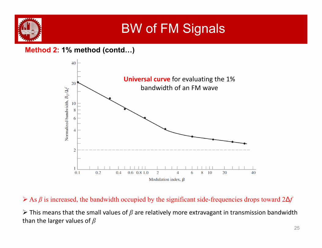
BW of FM SignalsMethod 2: 1% method (contd…)

U i l f l ti th 1%Universal curve for evaluating the 1% bandwidth of an FM wave

As β is increased, the bandwidth occupied by the significant side-frequencies drops toward 2Δf

25

β , p y g q p f

This means that the small values of β are relatively more extravagant in transmission bandwidth than the larger values of β

BW of FM Signals

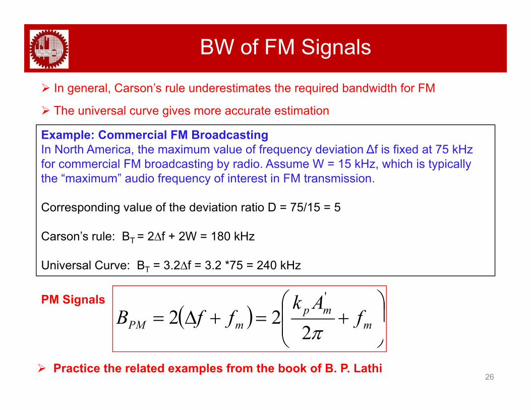
In general, Carson’s rule underestimates the required bandwidth for FM

The universal curve gives more accurate estimation

Example: Commercial FM BroadcastingIn North America, the maximum value of frequency deviation Δf is fixed at 75 kHz for commercial FM broadcasting by radio. Assume W = 15 kHz, which is typically the “maximum” audio frequency of interest in FM transmissionthe maximum audio frequency of interest in FM transmission.

Corresponding value of the deviation ratio D = 75/15 = 5

Carson’s rule: BT = 2∆f + 2W = 180 kHz

Universal Curve: BT = 3.2∆f = 3.2 *75 = 240 kHz

PM Signals

m

mpmPM f

AkffB

222

'

26 Practice the related examples from the book of B. P. Lathi

2

Generation and Demodulation of FM Signals

Modulators/Generators:

Varactor diode modulator

Reactance Modulator

Detectors/Demodulators:Detectors/Demodulators:

Foster-Seeley detector

Slope detector

27

Self-Study