· · 2016-05-27c811\01\007r rev o august 2002 page 0.1 of 0.3 us minerals management service...
TRANSCRIPT

C811\01\007R Rev O August 2002 Page 0.1 of 0.3
US MINERALS MANAGEMENT SERVICE1435-01-98-PO-16063
BEST PRACTICE FOR THE ASSESSMENT OF SPANS IN
EXISTING SUBMARINE PIPELINESVOLUME 2 - APPENDICES
C811\01\007R REV O AUGUST 2002
Purpose of Issue Rev Date of Issue Author Checked Approved
Final report O August 2002
JKS HMB HMB
Controlled Copy Uncontrolled Copy
BOMEL LIMITED
Ledger House
Forest Green Road, Fifield
Maidenhead, Berkshire
SL6 2NR, UK
Telephone +44 (0)1628 777707
Fax +44 (0)1628 777877
Email [email protected]

C811\01\007R Rev O August 2002 Page 0.2 of 0.3
CONTENTS
Page No.
VOLUME 1
EXECUTIVE SUMMARY 0.4
1. INTRODUCTION, BACKGROUND AND SCOPE OF WORK 1.1
1.1 INTRODUCTION 1.1
1.2 BACKGROUND 1.2
1.3 SCOPE OF WORK 1.3
2. APPROACHES TO SPAN ASSESSMENT 2.1
2.1 INTRODUCTION 2.1
2.2 PRINCIPAL CONSIDERATIONS 2.1
2.3 AVAILABLE APPROACHES 2.2
2.3.1 The Basic Approach 2.2
2.3.2 Screening Approach 2.4
2.3.3 The Tiered Approach 2.6
3. UNCERTAINTY 3.1
3.1 PREAMBLE 3.1
3.2 RISK AND RELIABILITY FUNDAMENTALS 3.4
3.2.1 Qualitative Indexing Systems 3.4
3.2.2 Quantitative Risk Systems 3.6
3.3 SPATIAL AND TEMPORAL VARIABILITY 3.10
4. DATA FOR SPAN ASSESSMENT 4.1
4.1 PREAMBLE 4.1
4.2 DATA CLASSES 4.1
4.3 DATA SOURCES 4.2
5. SURVEYS 5.1
5.1 PREAMBLE 5.1
5.2 SURVEY TECHNIQUES 5.1
6. ASSESSMENT BENCHMARKING 6.1
C811\01\007R Rev O August 2002 Page 0.3 of 0.3
7. DISCUSSION OF CURRENT PRACTICE 7.1
8. WAY FORWARD 8.1
9. REFERENCES 9.1
VOLUME 2
APPENDIX A - PIPELINE DEFECT ASSESSMENT PROCESS: SPAN ANALYSIS FOR STATIC STRENGTH
AT THE TIER 1 LEVEL
APPENDIX B - PIPELINE DEFECT ASSESSMENT PROCESS: SPAN ANALYSIS FOR STATIC STRENGTH
AT THE TIER 2 LEVEL
APPENDIX C - PIPELINE DEFECT ASSESSMENT PROCESS: SPAN ANALYSIS FOR STATIC STRENGTH
AT THE TIER 3 LEVEL
APPENDIX D - PIPELINE DEFECT ASSESSMENT PROCESS: SPAN ANALYSIS FOR DYNAMIC
OVERSTRESS AT THE TIER 1 LEVEL (VORTEX SHEDDING)
APPENDIX E - DEVELOPMENT OF FATIGUE ASSESSMENT METHODOLOGY
APPENDIX F - CRITERIA DETERMINING THE STATIC STRENGTH OF PIPELINE SPANS
APPENDIX G - RECOMMENDED INSPECTION STRATEGY
APPENDIX H - COPY OF REFERENCE: BOMEL, 1995

C811\01\007R Rev O August 2002 Page A.0.1 of A.0.4
APPENDIX A
PIPELINE DEFECT A SSESSMENT
PROCESS: SPAN ANALYSIS FOR
STATIC STRENGTH AT THE TIER 1
LEVEL

C811\01\007R Rev O August 2002 Page A.0.2 of A.0.4
TABLE OF CONTENTS
Page No
A.1
A.2
INTRODUCTION
A.1.1 PURPOSE
A.1.2 SCOPE AND LIMITATIONS
A.1.3 REFERENCES
A.1.3.1 Codes And Standards
PROCESS
A.2.1 OBJECTIVE
A.2.2 ASSESSMENT STRATEGY AT THE TIER 1 LEVEL
A.2.2.1 Generic
A.2.2.2 Considerations In The Tier 1 Static Strength Analytical
Method
A.2.3 DATA
A.2.3.1 Data Classes
A.2.3.2 Data Sources
A.2.4 LOADINGS AND LOAD COMBINATIONS IN GENERAL
A.2.4.1 General Points
A.2.4.2 Actions
A.2.4.3 Loadings
A.2.5 LOAD COMBINATION IN TIER 1 ANALYTICAL METHOD
A.2.5.1 Load Combination
A.2.5.2 Submerged Self-Weight
A.2.5.3 Environmental: Long-Term
A.2.5.4 Environmental: Short-Term
A.2.5.5 Operating
A.2.6 ANALYTICAL CRITERIA
A.2.6.1 General
A.2.6.2 Stress Criterion
A.2.6.3 Strain Criterion
A.2.6.4 Ovalisation Criterion
A.2.6.5 Local Buckling Criterion
A.2.7 TIER 1 STATIC STRENGTH ANALYTICAL METHOD
A.2.7.1 General
A.2.7.2 Loadings
A.2.7.3 Support Conditions
A.2.7.4 Material Characteristic
A.1.1
A.1.1
A.1.1
A.1.1
A.1.1
A.2.1
A.2.1
A.2.1
A.2.1
A.2.1
A.2.2
A.2.2
A.2.2
A.2.3
A.2.3
A.2.3
A.2.3
A.2.4
A.2.4
A.2.4
A.2.4
A.2.5
A.2.5
A.2.6
A.2.6
A.2.6
A.2.6
A.2.7
A.2.7
A.2.7
A.2.7
A.2.8
A.2.8
A.2.9
C811\01\007R Rev O August 2002 Page A.0.3 of A.0.4
TABLE OF CONTENTS/continued
A.2.7.5 Cross-section Bending Resistance A.2.9
A.2.7.6 Span Mechanical Model A.2.13
A.2.7.7 Analysis Procedure A.2.15
A.2.7.8 Analytical Method Implementation A.2.16
A.2.8 ACCEPTANCE CRITERION A.2.16
A.3 ATTACHMENTS A.3
C811\01\007R Rev O August 2002 Page A.0.4 of A.0.4
LIST OF TABLES
Table A.2.1 Data Classes
Table A.2.2 Relationship Between Actions, Loading And Load Combinations
Table A.2.2 Input And Response Parameters For Tier 1 Span Mechanical Model
Table A.3.1 Example Of Tier 1 Static Strength Analysis Proforma
LIST OF FIGURES
Figure A.2.1 Static Strength Assessment At The Tier 1 Level

C811\01\007R Rev O August 2002 Page A.1.1 of A.1.1
A.1 INTRODUCTION
A.1.1 PURPOSE
The purpose of this process is to set down the methodology for the static strength analysis of
pipeline spans at the Tier 1 level and to ensure that best practice is applied.
A.1.2 SCOPE AND LIMITATIONS
This process applies to pipelines laid directly onto the seabed. It applies to an individual span;
that is, a single clear unsupported length of pipeline that is sufficiently isolated from other spans
or features as to be judged to behave as a self-contained entity. It does not apply to pipelines
that are trenched, trenched and backfilled, trenched and infilled due to natural soil migration, or
pipelines that are piggybacked.
A.1.3 REFERENCES
A.1.3.1 Codes And Standards! Rules For Submarine Pipeline Systems. Det Norske Veritas. DNV, 1996.
! Code Of Practice For Pipelines Subsea: Design, Construction And Installation. British
Standards Institute (BSI). BS 8010: Part 3: 1993.
! American Petroleum Institute (API). Recommended Practice For Planning, Designing,
And Constructing Fixed Offshore Platforms - Working Stress Design. RP2A-WSD,
20th ed., July 1993.
C811\01\007R Rev O August 2002 Page A.2.1 of A.2.20
A.2 PROCESS
A.2.1 OBJECTIVE
The objective of this process is to ensure that the static strength analysis of pipeline spans at
the Tier 1 level is conducted in a rigorous manner, with due regard to the mechanical
characteristics of the problem, using appropriate analytical criteria, and that spans are
determined to be acceptable or significant against acceptance criteria.
A.2.2 ASSESSMENT STRATEGY AT THE TIER 1 LEVEL
A.2.2.1 GenericThe recommended Pipeline Defect Assessment Procedure allows a tiered approach to analytical
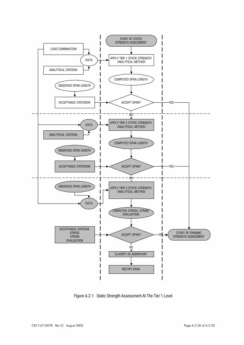
methods and span acceptance. Specifically, up to a three-tiered philosophy can be adopted
as shown in detail for the failure mode of static strength in Figure A.2.1. In this figure, the upper
level tiers have been greyed, leaving the Tier 1 assessment covered by this process highlighted.
At whatever tier level, the approach involves interaction between the data, load combination,
analytical criteria, analytical methods and acceptance criteria; each of these is dealt with in
detail in subsections A.2.3 to A.2.8, below. At Tier 1, observed span lengths are judged against
span lengths computed from the analytical method, using acceptance criteria, to determine
acceptability:
! data, load combinations and analytical criteria are all input into the analytical method
! output from the analytical method is a computed span length, which is compared with
the observed span length to determine acceptability of the latter using an acceptance
criterion.
A.2.2.2 Considerations In The Tier 1 Static Strength Analytical MethodFor the static strength analytical method recommended for pipeline spans in this process
document consideration should be given to the following factors:
! loadings
! support conditions
! material characteristic
! cross-section bending resistance
! span mechanical model
C811\01\007R Rev O August 2002 Page A.2.2 of A.2.20
! analysis procedure
! analytical method implementation.
Each of these points is addressed in detail in subsection A.2.7, below.
A.2.3 DATA
A.2.3.1 Data ClassesA detailed breakdown of the data into the four classes of: pipeline, operational, environmental
and inspection is given in Table 2.1. Data in the lines of Table 2.1 that have been greyed are
considered to be unnecessary to perform the Tier 1 static strength analysis. The remainder can
be viewed as “baseline” data, some of which have to be processed by means of calculation into
suitable input data for the analysis.
The pipeline data include geometrical and material properties; these are used in the analytical
model, the analytical criteria and the material characteristic. The axial restraint factor is used
to approximate the degree of suppression of longitudinal strains in the pipe wall due to the
interaction of the pipe with the seabed.
The operational data encompass installation (residual lay tension) and those related to the pipe
contents: its density, pressure and temperature; these are used to derive some of the loadings
applied to the span.
The environmental data include the parameters that relate to the fluid loading on the pipeline
(for example, water depth and various wave and current data). They also contain parameters
defining the mechanical interaction between the pipe and the seabed (for example, soil modulus
and Poisson’s ratio at the span shoulders); these particular parameters influence the suppor t
conditions at the shoulder of the pipeline.
The inspection data include parameters to locate the span (kilometre start and end points), and
freespan length. If marine growth information is included within the inspection data an
assessment should be made as to whether this influences the pipeline weight or the
hydrodynamic loading on the pipeline.
A.2.3.2 Data SourcesAppropriate sources of pipeline, operational and environmental data are to be used. If no data
are available for residual lay tension or axial restraint factor, then these are to be estimated
conservatively and included if they adversely affect the pipeline.
C811\01\007R Rev O August 2002 Page A.2.3 of A.2.20
A.2.4 LOADINGS AND LOAD COMBINATIONS IN GENERAL
A.2.4.1 General PointsA load combination is built up from actions and loadings as shown schematically in Table A.2.2.
The loading combination to be used is a requirement of the assessment and, as indicated in
subsection A.2.5, an operating loading is always included in the combination. This will usually
correspond to the normal operating conditions of the pipeline, although there may be occasions
where other operating conditions need to be considered.
A.2.4.2 ActionsIn terms of detailed thermo-mechanical actions there are eight types that require consideration:
! pipeline weight
! external temperature
! external pressure
! current-induced action
! wave-induced action
! contents weight
! internal temperature
! internal pressure.
A.2.4.3 LoadingsFour individual loading classes are to be considered, namely:
! submerged self weight
! environmental: long-term
! environmental: short-term
! operating.
More than one type of operating condition may need to be addressed. As indicated in Table
A.2.2, the list covers the following possibilities:
! normal operating
! maximum allowable operating
! shut down (minimum operating)
! hydrotest.
This list may be extended if circumstances dictate.
C811\01\007R Rev O August 2002 Page A.2.4 of A.2.20
q q q q qs e c a= + + −
( )[ ]ss
qg
D D t= − −ρ π
422 2
( )ee
eqg
D t D= + −
ρ π
42
2 2
( ) ( )cc
e c eqg
D t t D t= + + − +
ρ π
42 2 2
2 2
( )aa
e cqg
D t t= + +ρ π
42 2
2
a ap gh= ρ
A.2.5 LOAD COMBINATION IN TIER 1 ANALYTICAL METHOD
A.2.5.1 Load CombinationA load combination is made up from loading classes, and will always comprise the submerged
self-weight, environmental long- and shor t-term load and an operating class, as set out
schematically in Table A.2.2.
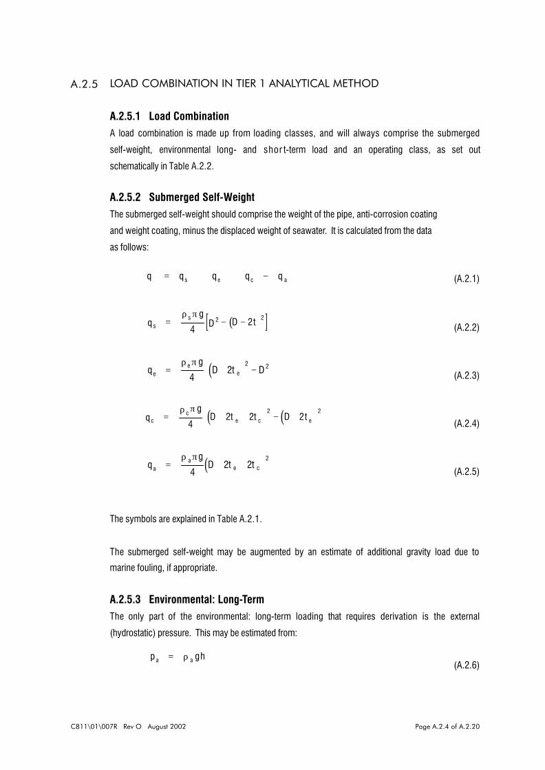
A.2.5.2 Submerged Self-WeightThe submerged self-weight should comprise the weight of the pipe, anti-corrosion coating
and weight coating, minus the displaced weight of seawater. It is calculated from the data
as follows:
(A.2.1)
(A.2.2)
(A.2.3)
(A.2.4)
(A.2.5)
The symbols are explained in Table A.2.1.
The submerged self-weight may be augmented by an estimate of additional gravity load due to
marine fouling, if appropriate.
A.2.5.3 Environmental: Long-TermThe only part of the environmental: long-term loading that requires derivation is the external
(hydrostatic) pressure. This may be estimated from:
(A.2.6)

C811\01\007R Rev O August 2002 Page A.2.5 of A.2.20
( ) ( )h a d e c c wq C D t t V V= + + +12
2 22
ρ
( )iiq
gD t= −
ρ π
42 2
A.2.5.4 Environmental: Short-TermThe environmental: short-term loading comprises the hydrodynamic uniformly distributed load
resulting from the drag on the pipeline from the moving water par ticle velocities. Inertia loading
is generally small, and in most circumstances may be neglected. It is recommended that
directional 50-year return period maximum wave height and period (Hmax and Tmax), and
associated maximum surface current velocity are used to determine the maximum combined
water particle velocity normal to the heading of the span, which forms the input to Morison’s
equation to derive the loading on the span. The main steps in this process are as follows:
1. Use directional 50-year return period maximum wave height and period (Hmax and
Tmax), and associated maximum surface current velocity
2. Considering the heading of the pipeline span, determine the maximum wave height
and corresponding period, and associated surface current velocity normal to the
pipeline span
3. Compute the top-of-pipe current velocity Vc using a power-law current profile
suggested in the source data
4. Compute the top-of-pipe maximum wave velocity Vw using a wave theory suitable for
the Hmax - Tmax - water depth combination concerned (kinematic spreading may be
neglected, and the effect of current velocity on wave period may be ignored)
5. The uniformly distributed load is then derived from:
(A.2.7)
The environmental: short-term loading may be augmented by an estimate of additional load due
to marine fouling, if required.
A.2.5.5 OperatingThe only par t of the operating loading that requires derivation is the contents self-weight. This
is given by:
(A.2.8)
C811\01\007R Rev O August 2002 Page A.2.6 of A.2.20
A.2.6 ANALYTICAL CRITERIA
A.2.6.1 GeneralIt is recommended that the static strength analytical criteria should embody:
! stress limits
! plastic strain limits
! ovalisation limits
! limits derived from local buckling considerations.
The choice and use of criteria are set out below, and their precise implementation within the
analytical method is dealt with in subsection A.2.7, below.
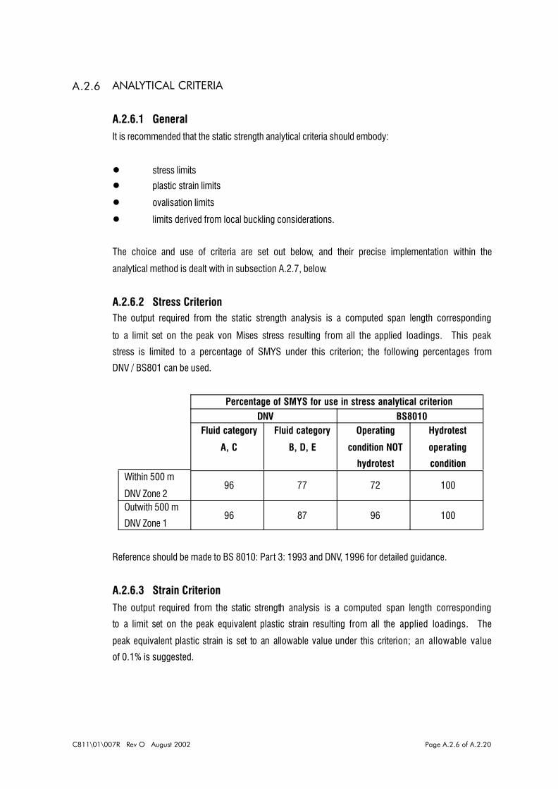
A.2.6.2 Stress CriterionThe output required from the static strength analysis is a computed span length corresponding
to a limit set on the peak von Mises stress resulting from all the applied loadings. This peak
stress is limited to a percentage of SMYS under this criterion; the following percentages from
DNV / BS801 can be used.
Percentage of SMYS for use in stress analytical criterionDNV BS8010
Fluid category
A, C
Fluid category
B, D, E
Operating
condition NOT
hydrotest
Hydrotest
operating
conditionWithin 500 m
DNV Zone 296 77 72 100
Outwith 500 m
DNV Zone 196 87 96 100
Reference should be made to BS 8010: Part 3: 1993 and DNV, 1996 for detailed guidance.
A.2.6.3 Strain CriterionThe output required from the static strength analysis is a computed span length corresponding
to a limit set on the peak equivalent plastic strain resulting from all the applied loadings. The
peak equivalent plastic strain is set to an allowable value under this criterion; an allowable value
of 0.1% is suggested.

C811\01\007R Rev O August 2002 Page A.2.7 of A.2.20
( )max min .5%D D
DOOR
−≤ −
21
A.2.6.4 Ovalisation CriterionThe output required from the static strength analysis is a computed span length corresponding
to a limit set on the peak cross-section ovalisation resulting from the applied loadings. The peak
ovalisation is set to an allowable value under this criterion. It is suggested that an allowable
value of 1.5%, corrected for the out-of-roundness (OOR) tolerance from fabrication of the pipe,
is used giving a criterion as follows:
(A.2.9)
where Dmax and Dm i n are the maximum and minimum diameters, respectively, on the most highly
ovalised cross-section.
Given that internal pressure has an ameliorating effect on ovalisation, consideration should be
given to a load combination that excludes internal pressure.
A.2.6.5 Local Buckling CriterionThis is related to the collapse of the cross-section. The output required from the static strength
analysis is a computed span length such that local buckling of the most highly bent cross-
section does not occur under the applied loadings. The peak bending strain is set to an
allowable value under this criterion.
Given that internal pressure has an ameliorating effect on local buckling, consideration should
be given to a load combination that excludes internal pressure.
A.2.7 TIER 1 STATIC STRENGTH ANALYTICAL METHOD
A.2.7.1 GeneralThe static strength analytical method for implementation at the Tier 1 level uses a strain-based
approach, consisting of three aspects:
! a cross-section bending resistance model based on an additional plastic strain
limitation
! a span mechanical model that explicitly embodies span end conditions and the exact
effects of effective axial force
! an analysis procedure that links the resistance and mechanical models together.
Each of these aspects is dealt with in detail in subsections A.2.7.5, A.2.7.6 and A.2.7.7, below.

C811\01\007R Rev O August 2002 Page A.2.8 of A.2.20
( )vf
f
kE
=−2 1 2ν
( )hf
f
kE
=+2 1 ν
A.2.7.2 LoadingsThe loadings that should be applied in the analytical method are as follows:
! prestressing due to residual lay tension (to be estimated conservatively and included
if it adversely affects the pipeline)
! internal temperature q i
! internal pressure pi (which may be the normal operating, maximum allowable
operating or hydrotest pressure, whichever is under attention; consideration should
also be given to omitting the internal pressure if this is appropriate to the analytical
criterion under use, see subsection 2.6)
! external temperature qa
! external pressure pa (see subsection A.2.5.3, above)
! total vertical uniformly distributed load qv = q + qi (see subsections A.2.5.2 and
A.2.5.5, above)
! total horizontal uniformly distributed load qh (see subsection A.2.5.4, above).
A.2.7.3 Support ConditionsSymmetry at midspan may be assumed. In this case, appropriate symmetry boundary
conditions on displacement are enforced at midspan, and one shoulder region considered.
Regarding the shoulder region, consideration must be given to support conditions in the vertical
and transverse-horizontal directions. In the present case it is recommended that the supports
are modelled as continuous elastic foundations in the ver tical and transverse-horizontal planes
to represent deformability of the seabed and its interaction with the pipe.
For elastic constants to be used in these types of support it is suggested that the stiffness per
unit length of the vertical support should be derived as follows:
(A.2.10)
and the stiffness per unit length of the transverse-horizontal support should be derived as
follows:
(A.2.11)
It is in order to use a planar value of transverse stiffness per unit length as the resultant of the
above two, i.e.

C811\01\007R Rev O August 2002 Page A.2.9 of A.2.20
k k kf v h= +2 2(A.2.12)
A.2.7.4 Material CharacteristicThe stress-strain characteristic for the pipeline steel should be taken as elastic-perfectly plastic,
with Young’s modulus of E, Poisson’s ratio of ν and yield strength of σo.
A.2.7.5 Cross-section Bending ResistancePhysical Model. The cross-section bending resistance model computes an allowable bending
moment for a given pipe cross-section (outside diameter and wall thickness), material, subject
to pressure and thermal loadings; the resistance is subject to a prescribed limit on maximum
strain derived from the analytical criterion. This limit may be elastic (whereupon the allowable
bending moment relates to a standard stress limit), or based on an equivalent plastic strain
criterion; it is thus completely general.
The mathematical modelling is based on an analysis that is separated out into two phases, as
follows:
! prebending analysis, in which the pipeline is fully supported in the vertical and
transverse-horizontal directions along its full length by the seabed, and thus involves
no bending
! bending analysis, which models the state of stress within the pipeline as a result of
spanning, and thus involves bending.
Assumptions. The assumptions used in both phases of the analysis are as follows:
1. The contribution of any weight and/or anti-corrosion coat to stiffness and strength of
the pipeline cross-section is ignored.
2. The uniaxial stress-strain response of the pipe steel is elastic-perfectly plastic and
material yield is governed by the von Mises yield criterion.
3. Pipe steel plasticity is governed by the Reuss equations for incremental plasticity.
4. Membrane thin-shell calculations based on the pipe median sur face are sufficiently
accurate for stresses in the pipe wall, with plane stress assumptions taken with
respect to the through-thickness direction.
5. Plane cross-sections of the pipe remain plane af ter bending.
Prebending Analysis. This analysis comprises the loading due to internal and external
pressure, internal and external temperature, and axial forces due to restrained longitudinal
expansion and residual lay tension. The objectives are to determine:

C811\01\007R Rev O August 2002 Page A.2.10 of A.2.20
( ) ( )σ θ = −
−p p
D t
ti a 2
( ){ }σ λ νσ α θ θθxs
a i aN
AE= + − −
( ){ }N N A Enetx a s i a= + − −λ ν σ α θ θθ
( )[ ]A D D ts = − −π4
22 2
( ) ( )ε σ ν σ α θ θθ θ= − + −1E x i a
( ) ( )ε σ νσ α θ θθx x i aE= − + −
1
σ σ σ σθ θyxt o= + −
12
4 32 2
σ σ σ σθ θyxc o= − −
12
4 32 2
( ) ( )ε σ νσ α θ θθyxt yxt i aE= − + −
1
( ) ( )ε σ ν σ α θ θθyxc yxc i aE= − + −
1
! the state of stress and strain in the pipe and the net axial force
! the state of stress and strain necessary to just yield the pipe.
The prebending stresses in the pipe will be given by the following formulae:
(A.2.13)
(A.2.14)
and the net axial force is
(A.2.15)
where
(A.2.16)
The corresponding strains are given by:
(A.2.17)
(A.2.18)
The longitudinal stresses at yield for a prescribed hoop stress, from the von Mises ellipse, are
as follows:
(A.2.19)
(A.2.20)
and the corresponding longitudinal strains are:
(A.2.21)
(A.2.22)
C811\01\007R Rev O August 2002 Page A.2.11 of A.2.20
ε ε σσ ε
σσ
σ
ε ε σσ ε
σσ
σ
θ θ
θ θ
fx yxt yxt
p
ox
fx yxc yxc
p
ox
dif or
dif
= + −
>
= + −
≤
2 2
2 2
ε ε ε σσ
ε ε ε σσ
θ
θ
fx x b x
fx x b x
if or
if
= + >
= − ≤
2
2
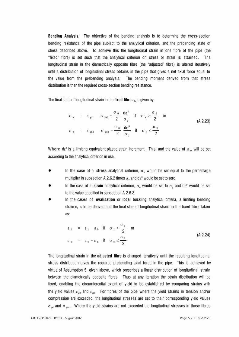
Bending Analysis. The objective of the bending analysis is to determine the cross-section
bending resistance of the pipe subject to the analytical criterion, and the prebending state of
stress described above. To achieve this the longitudinal strain in one fibre of the pipe (the
“fixed” fibre) is set such that the analytical criterion on stress or strain is attained. The
longitudinal strain in the diametrically opposite fibre (the “adjusted” fibre) is altered iteratively
until a distribution of longitudinal stress obtains in the pipe that gives a net axial force equal to
the value from the prebending analysis. The bending moment derived from that stress
distribution is then the required cross-section bending resistance.
The final state of longitudinal strain in the fixed fibre εfx is given by:
(A.2.23)
Where dεp is a limiting equivalent plastic strain increment. This, and the value of σo, will be set
according to the analytical criterion in use.
! In the case of a stress analytical criterion, σo would be set equal to the percentage
multiplier in subsection A.2.6.2 times σy and dεp would be set to zero.
! In the case of a strain analytical criterion, σo would be set to σy and dεp would be set
to the value specified in subsection A.2.6.3.
! In the cases of ovalisation or local buckling analytical criteria, a limiting bending
strain eb is to be derived and the final state of longitudinal strain in the fixed fibre taken
as:
(A.2.24)
The longitudinal strain in the adjusted fibre is changed iteratively until the resulting longitudinal
stress distribution gives the required prebending axial force in the pipe. This is achieved by
virtue of Assumption 5, given above, which prescribes a linear distribution of longitudinal strain
between the diametrically opposite fibres. Thus at any iteration the strain distribution will be
fixed, enabling the circumferential extent of yield to be established by comparing strains with
the yield values εyxt and εyxc. For fibres of the pipe where the yield strains in tension and/or
compression are exceeded, the longitudinal stresses are set to their corresponding yield values
σyxt and σ yxc . Where the yield strains are not exceeded the longitudinal stresses in those fibres

C811\01\007R Rev O August 2002 Page A.2.12 of A.2.20
are set from elastic considerations. In this way the distribution of longitudinal stress around the
circumference of the pipe is established and integration of this over the cross-section area gives
a net axial force that is compared with the prebending value. Once convergence to the required
axial force is attained, the longitudinal strain and stress distributions are completely defined,
enabling the cross-section bending resistance to be computed by integration.
Calculation Procedure. The calculation procedure for the cross-section bending resistance is
iterative. It is judged to be more practical to implement one calculation procedure for stress or
strain analytical criteria, despite the fact that for stress criteria elastic response results and an
iterative procedure is not, strictly speaking, necessary. The steps that need to be followed to
perform the calculation are as follows:
1. Compute the prebending stresses and strains in the pipe, and the net axial force.
2. Compute the total longitudinal stresses at yield using the von Mises ellipse, and their
corresponding strains.
3. Compute the bending stresses and corresponding bending strains necessar y to cause
yield.
4. Set the longitudinal strain in the fixed fibre by either:
4a. Select the bending strain that causes first yield, add this to the prebending
longitudinal strain and assign the result to the fixed fibre and
4b. Calculate the longitudinal plastic strain increment from the stresses at yield
of the fixed fibre and the analytical criterion being enforced and
4c. Add to the strain at first yield in the fixed fibre from Step 3, the longitudinal
plastic strain increment from Step 4.b to give the total limiting strain in the
fixed fibre;
or add the bending strain corresponding to the analytical criterion to the prebending strain, and
assign the result to the fixed fibre.
5. Guess a total longitudinal strain for the adjusted fibre and assume a linear longitudinal
strain variation across the pipe diameter between this and the fixed fibre.
6. Compare the strain distribution from Step 5 with the yield strains from Step 2 to
deduce the longitudinal stress distribution, including the extent of plasticity.
7. Calculate the net axial force in the pipe wall by integration of the longitudinal stress

C811\01\007R Rev O August 2002 Page A.2.13 of A.2.20
( )EI
E I s* =−1 2ν
( )[ ]I D D ts = − −π64
24 4
( )
( )
N A p D t if
N p D t if
a x s i x
a i x
= − − ≤
= − − >
σπ
σ
πσ
42 0
42 0
2
2
q q qn v h= +2 2
distribution from Step 6 (with due regard to the extent of plasticity); if this does not
agree with that from Step 1, iterate through Step 5 et seq.
8. Calculate the cross-section bending resistance in the pipe by product integration of
the longitudinal stress distribution from Step 6 (with due regard to the extent of
plasticity).
A.2.7.6 Span Mechanical ModelSpan idealisation. The pipeline span is idealised as an infinitely long beam on a Winkler-type
elastic foundation, in which a central portion of the elastic foundation has been removed, leaving
a freespan. The loading comprises a uniformly distributed load and an axial compressive force
(the effective axial force). In general, deflections (normal to the pipe axis) will occur over the
full length of the pipe but will attenuate within the elastically-supported parts (the shoulders)
at rate that depends on the elastic foundation stiffness per unit length and the pipe bending
rigidity.
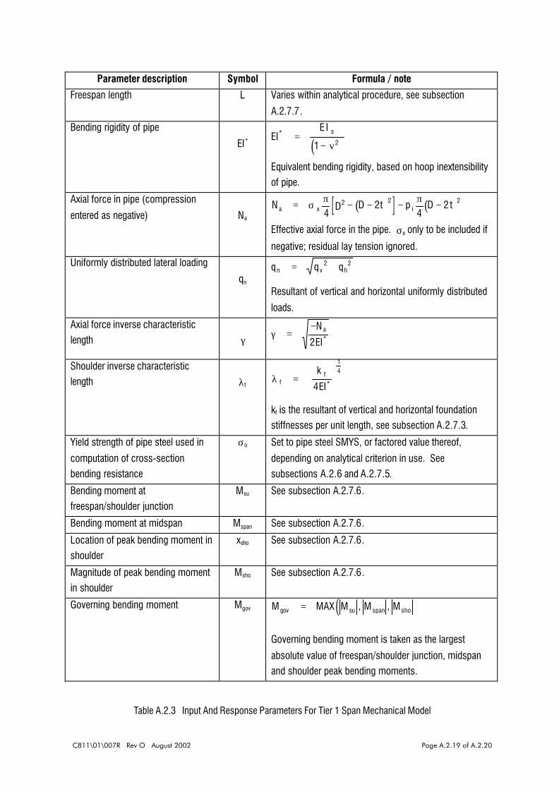
Problem parameters. The model input and response parameters are summarised in Table
A.2.3. The input parameters are L, EI*, Na, qn, g and lf and the response parameters are Msu,
Mspan, xsho, Msho and Mgov.
Some of the input parameters are computed from baseline data as follows:
Equivalent bending rigidity of the pipe EI*:
(A.2.25)
where
(A.2.26)
Effective axial compression in pipe Na:
(A.2.27)
Uniformly distributed lateral loading qn:
(A.2.28)

C811\01\007R Rev O August 2002 Page A.2.14 of A.2.20
γ =−N
EIa
2 *
λ ffk
EI=
4
14
*
Lf
<
−
−211
2
γγ
λcos
( ){ }( )
( )( )
q
N
L LM
N
L
L
q L M
EI
n
asu
a
n su f
f f
2 2 2
2 2 1
2
4
2 30
2 2
γ
γ γ γ γ
γ
α
α β
tancos
sin
*
−
−−
+
+−
−=
α ff ak
EI
N
EI= +
4 4* *
β ff ak
EI
N
EI= −
4 4* *
Axial force inverse characteristic length γ:
(A.2.29)
Shoulder inverse characteristic length λf:
(A.2.30)
Expressions for the various response bending moments are dealt with below.
Bar-buckling and upper range of limiting span length. Owing to the possibility of bar-buckling
of the span due the compression caused by the effective axial force, there exists an upper limit
to allowable span length that will be determined by this phenomenon. This may be found from
the following equation:
(A.2.31)
Bending moment at freespan/shoulder junction Msu. The bending moment at the junction
between the freespan and the shoulder (i.e. at the end of the span) is determined from:
(A.2.32)
where
(A.2.33)
(A.2.34)

C811\01\007R Rev O August 2002 Page A.2.15 of A.2.20
( )Mq
LM
LL
Lspan
nsu=
−
+
−
21
2
1 22
1 222γ γ
γγ
γcoscos
tan
tan
( ) ( )( )cot β
β α
α βf sho
f su f x
f su f x
xM M
M M=
− +
−
( )( )M
q L Mx
n f f f f su
f f f
=+ −
− −
λ α α β
β α β
2 2 2
2 2
3
3
M M Msho = +3 4
( )( ) ( )M
q Le xn
f
f
f f
xf sho
f sho3
2
2 23=
−
−−
βλ
α ββα sin
( ) ( ) ( )( ) ( )M M e x xsu
xf sho
f f f
f f ff sho
f sho4
2 2
2 2
3
3= −
−
−
−α βα α β
β α ββcos sin
( )M MAX M M Mgov su span sho= , ,
Bending moment at midspan Mspan. The bending moment at midspan is given by:
(A.2.35)
Location and magnitude of peak bending moment in shoulder xsho and Msho. The location of the
peak bending moment in the shoulder portion of the pipe is found from:
(A.2.36)
(A.2.37)
and the magnitude of the corresponding bending moment is computed from:
(A.2.38)
where
(A.2.39)
(A.2.40)
Governing bending moment Mgov. The governing bending moment in the model is taken as the
largest absolute value of the three bending moments given above, as follows:
(A.2.41)
A.2.7.7 Analysis ProcedureIn the analysis procedure, the span length is determined for which the governing bending
moment from the span mechanical model equals the allowable bending moment from the cross-
section bending resistance model. In cases where the allowable bending moment corresponds
with a stress analytical criterion, this relates to an exact elastic technique. For situations where

C811\01\007R Rev O August 2002 Page A.2.16 of A.2.20
L Lobs comp≤ 0 9.
a plastic strain limit is used (as determined from strain, ovalisation, or local buckling analytical
criteria), the approach corresponds to a lower-bound equilibrium technique. This is because of
the three necessary and sufficient conditions for the collapse of a structure:
! equilibrium is satisfied because the system of bending moments selected for the
analysis is in equilibrium with the imposed loads
! yield is satisfied because the governing bending moment does not exceed the fully
plastic moment of the pipe
! the mechanism criterion is violated because insufficient plastic hinges are present
in the pipe for a mechanism to occur.
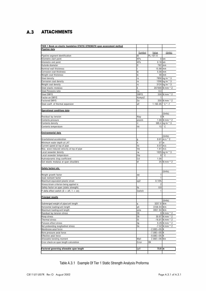
A.2.7.8 Analytical Method ImplementationThe analytical method has been implemented into a spreadsheet program. An example of an
analysis proforma is given in Section A.3, ATTACHMENTS.
A.2.8 ACCEPTANCE CRITERION
The output from the Tier 1 static strength analysis method is a computed span length Lcomp. A
percentage of this is compared with the observed span length to determine acceptability of the
latter; the percentage suggested is 90%. Hence, the criterion for acceptability of the observed
span is:
(A.2.42)

C811\01\007R Rev O August 2002 Page A.2.17 of A.2.20
Data Symbol
Pipeline DataPipe outside diameter D
Pipe nominal wall thickness t
Corrosion coat thickness teWeight coat thickness tcSteel density ρs
Corrosion coat density ρe
Weight coat density ρc
Steel elastic modulus E
Steel Poisson’s ratio ν
SMYS steel σy
Steel thermal expansion coefficient α
Axial restraint factor λa
Pipeline heading ϕ
Operational Data
Residual lay tension NInternal pressure pi
Contents density ρi
Contents temperature θi
Design life of pipeline Tp
Environmental Data
Minimum water depth at LAT h
Local seawater density ρa
Local seawater temperature θa
Current velocity data -
Wave data -
Hydrodynamic drag coefficient Cd
Hydrodynamic added mass coefficient Ca
Soil elastic modulus at span shoulders Ef
Soil Poisson’s ratio at span shoulders νf
Longitudinal friction coefficient at span shoulders µL
Transverse friction coefficient at span shoulders µT
Inspection Data
Kilometre point at start of span KPs
Kilometre point at end of span KPe
Freespan length Lobs
Gap beneath span G
Marine growth information -
Table A.2.1 Data Classes

C811\01\007R Rev O August 2002 Page A.2.18 of A.2.20
Action Loading Load Combination
PIPELINE WEIGHT SUBMERGED SELF-WEIGHT • • • •EXTERNAL TEMPERATURE ENVIRONMENTAL: LONG-TERM • • • •
EXTERNAL PRESSURE • • • •CURRENT-INDUCED ENVIRONMENTAL: SHORT-TERM • • • •
WAVE-INDUCED • • • •CONTENTS WEIGHT •
INTERNAL TEMPERATURE NORMAL OPERATING •INTERNAL PRESSURE •CONTENTS WEIGHT •
INTERNAL TEMPERATURE MAXIMUM ALLOWABLE
OPERATING•
INTERNAL PRESSURE •CONTENTS WEIGHT •
INTERNAL TEMPERATURE SHUT-DOWN (MINIMUM
OPERATING)•
INTERNAL PRESSURE •CONTENTS WEIGHT •
INTERNAL TEMPERATURE HYDROTEST •INTERNAL PRESSURE •
Table A.2.2 Relationship Between Actions, Loading And Load Combinations
C811\01\007R Rev O August 2002 Page A.2.19 of A.2.20
Parameter description Symbol Formula / note
Freespan length L Varies within analytical procedure, see subsection
A.2.7.7.
Bending rigidity of pipe
EI* ( )EI
E I s* =−1 2ν
Equivalent bending rigidity, based on hoop inextensibility of pipe.
Axial force in pipe (compression
entered as negative)
Na ( )[ ] ( )N D D t p D ta x i= − − − −σ
π π4
24
22 2 2
Effective axial force in the pipe. σx only to be included if
negative; residual lay tension ignored.
Uniformly distributed lateral loading
qn
q q qn v h= +2 2
Resultant of vertical and horizontal uniformly distributed
loads.
Axial force inverse characteristic length
γ
γ =−N
EIa
2 *
Shoulder inverse characteristic length
λf λ ffk
EI=
4
14
*
kf is the resultant of vertical and horizontal foundation stiffnesses per unit length, see subsection A.2.7.3.
Yield strength of pipe steel used in
computation of cross-section bending resistance
σo Set to pipe steel SMYS, or factored value thereof,
depending on analytical criterion in use. See subsections A.2.6 and A.2.7.5.
Bending moment at freespan/shoulder junction
Msu See subsection A.2.7.6.
Bending moment at midspan Mspan See subsection A.2.7.6.
Location of peak bending moment in shoulder
xsho See subsection A.2.7.6.
Magnitude of peak bending moment in shoulder
Msho See subsection A.2.7.6.
Governing bending moment Mgov ( )M MAX M M Mgov su span sho= , ,
Governing bending moment is taken as the largest
absolute value of freespan/shoulder junction, midspan and shoulder peak bending moments.
Table A.2.3 Input And Response Parameters For Tier 1 Span Mechanical Model
C811\01\007R Rev O August 2002 Page A.2.20 of A.2.20
ACCEPT SPAN?
DATA
ANALYTICAL CRITERIA
LOAD COMBINATION
APPLY TIER 1 STATIC STRENGTHANALYTICAL METHOD
COMPUTED SPAN LENGTH
OBSERVED SPAN LENGTH
YES
NO
ACCEPT SPAN?
APPLY TIER 2 STATIC STRENGTHANALYTICAL METHOD
COMPUTED SPAN LENGTH
YES
NO
ACCEPTANCE CRITERION
ACCEPT SPAN?
APPLY TIER 3 STATIC STRENGTHANALYTICAL METHOD
COMPUTED STRESS, STRAINOVALISATION
YES
NO
START OF DYNAMICSTRENGTH ASSESSMENT
CLASSIFY AS SIGNIFICANT
DATA
ACCEPTANCE CRITERIA:STRESSSTRAIN
OVALISATION
DATA
ANALYTICAL CRITERIA
ACCEPTANCE CRITERION
RECTIFY SPAN
START OF STATICSTRENGTH ASSESSMENT
OBSERVED SPAN LENGTH
OBSERVED SPAN LENGTH
Figure A.2.1 Static Strength Assessment At The Tier 1 Level
C811\01\007R Rev O August 2002 Page A.3.1 of A.3.1
TIER 1 Beam on elastic foundation STATIC STRENGTH span assessment methodPipeline data- Symbol Value (Units)Pipeline segment identification ID PL-101-AKilometre start point KPs 0 kmKilometre end point KPe 0.16 kmOutside diameter D 762 mmNominal wall thickness t 15.88 mmCorrosion coat thickness te 5.56 mmWeight coat thickness tc 48 mmSteel density rs 7850 kg/m^3Corrosion coat density re 1200 kg/m^3Weight coat density rc 3124 kg/m^3Steel elastic modulus E 207000 N/mm^2Steel Poissons ratio nu 0.3Steel SMYS SMYS 358 N/mm^2Factor on SMYS Ksmys2 1Factored SMYS So 358 N/mm^2Steel coeff. of thermal expansion alf 1.16E-05 ° C^-1
Operational conditions data- (Units)Residual lay tension Nlay 0 NContents pressure pnorm 1.69 N/mm^2Contents density ri 585.4 kg/m^3Contents temperature thi 15 ° C
Environmental data- (Units)Gravitational acceleration g 9.81 m/s^2Minimum water depth at LAT h 37 mCurrent speed at top of pipe Vc 0.57 m/sMax. wave induced velocity at top of pipe Vw 1.61 m/sLocal seawater density rw 1025 kg/m^3Local seawater temperature tha 8 ° CHydrodynamic drag coefficient Cd 1.05Soil elastic modulus at span shoulders kf 25 N/mm^2
Safety factors etc.- (Units)Weight growth factor ew 1Axial restraint factor l 1Maximum equivalent plastic strain ep2 0.10%Stress/strain criterion being applied is 2Safety factor on span (static strength) lls 0.9P-delta effect switch (0 = off, 1 = on) Switch 1
Principal results- (Units)Submerged weight of pipe/unit length q 3257.9 N/mHorizontal loading/unit length qh 2236.94 N/mMaximum loading/unit length qmx 3951.94 N/mResidual lay tension stress Slt 0 N/mm^2Hoop stress Sh 30.97 N/mm^2Thermal stress St -16.81 N/mm^2Poisson effect stress Sp 9.29 N/mm^2Net prebending longitudinal stress Sn -7.52 N/mm^2Membrane axial force -2.80E+05 NBore pressure axial force -7.08E+05 NEffective axial force -9.88E+05 NAllowable bending moment Mall 2.86E+06 NmError check on span length calculation Error OK
Factored governing allowable span length Ls1 73.9 m
A.3 ATTACHMENTS
Table A.3.1 Example Of Tier 1 Static Strength Analysis Proforma

C811\01\007R Rev O August 2002 Page B.0.1 of B.0.3
APPENDIX B
PIPELINE DEFECT A SSESSMENT
PROCESS: SPAN ANALYSIS FOR
STATIC STRENGTH AT THE TIER 2
LEVEL

C811\01\007R Rev O August 2002 Page B.0.2 of B.0.3
TABLE OF CONTENTSPage No.
B.1
B.2
B.3
INTRODUCTION
B.1.1 PURPOSE
B.1.2 SCOPE AND LIMITATIONS
B.1.3 REFERENCES
B.1.3.1 Codes And Standards
PROCESS
B.2.1 OBJECTIVE
B.2.2 ASSESSMENT STRATEGY AT THE TIER 2 LEVEL
B.2.2.1 Generic
B.2.2.2 Considerations In The Tier 2 Static Strength Analytical Method
B.2.3 DATA
B.2.3.1 Data Classes
B.2.3.2. Data Sources
B.2.4 LOADINGS AND LOAD COMBINATIONS IN GENERAL
B.2.4.1 General Points
B.2.4.2 Actions
B.2.4.3 Loadings
B.2.5 LOAD COMBINATION IN TIER 2 ANALYTICAL METHOD
B.2.5.1 Load Combination
B.2.5.2 Submerged Self-Weight
B.2.5.3 Environmental: Long-Term
B.2.5.4 Environmental: Short-Term
B.2.5.5 Operating
B.2.6 ANALYTICAL CRITERIA
B.2.6.1 General
B.2.6.2 Stress Criterion
B.2.7 TIER 2 STATIC STRENGTH ANALYTICAL METHOD
B.2.7.1 General
B.2.7.2 Loadings
B.2.7.3 Support Conditions
B.2.7.4 Material Characteristic
B.2.7.5 Mechanical Model
B.2.7.6 Analytical Method Implementation
B.2.8 ACCEPTANCE CRITERION
ATTACHMENTS
B.1.1
B.1.1
B.1.1
B.1.1
B.1.1
B.2.1
B.2.1
B.2.1
B.2.1
B.2.1
B.2.2
B.2.2
B.2.2
B.2.3
B.2.3
B.2.3
B.2.3
B.2.4
B.2.4
B.2.4
B.2.4
B.2.5
B.2.5
B.2.6
B.2.6
B.2.6
B.2.6
B.2.6
B.2.7
B.2.8
B.2.9
B.2.9
B.2.13
B.2.13
B.3.1

C811\01\007R Rev O August 2002 Page B.0.3 of B.0.3
LIST OF TABLES
Table B.2.1 Data Classes
Table B.2.2 Relationship Between Actions, Loading And Load Combinations
Table B.3.1 Example Of Tier 2 Static Strength Analysis Proforma
LIST OF FIGURES
Figure B.2.1 Static Strength Assessment At The Tier 2 Level
Figure B.2.2 Schematic Representation Of Tier 2 Analytical Method

C811\01\007R Rev O August 2002 Page B.1.1 of B.1.1
B.1 INTRODUCTION
B.1.1 PURPOSE
The purpose of this process is to set down the methodology for the static strength analysis of
pipeline spans at the Tier 2 level and to ensure that best practice is applied.
B.1.2 SCOPE AND LIMITATIONS
This process applies to pipelines laid directly onto the seabed. It applies to an individual span;
that is, a single clear unsupported length of pipeline that is sufficiently isolated from other spans
or features as to be judged to behave as a self-contained entity. It does not apply to pipelines
that are trenched, trenched and backfilled, trenched and infilled due to natural soil migration, or
pipelines that are piggybacked.
B1.3 REFERENCES
B1.3.1 Codes And Standards! Rules For Submarine Pipeline Systems. Det Norske Veritas. DNV, 1996.
! Code Of Practice For Pipelines Subsea: Design, Construction And Installation. British
Standards Institute (BSI). BS 8010: Part 3: 1993.
! American Petroleum Institute (API). Recommended Practice For Planning, Designing,
And Constructing Fixed Offshore Platforms - Working Stress Design. RP2A-WSD,
20th ed., July 1993.
C811\01\007R Rev O August 2002 Page B.2.1 of B.2.17
B.2 PROCESS
B.2.1 OBJECTIVE
The objective of this process is to ensure that the static strength analysis of pipeline spans at
the Tier 2 level is conducted in a rigorous manner, with due regard to the mechanical
characteristics of the problem, using appropriate analytical criteria, and that spans are
determined to be acceptable or significant against acceptance criteria.
B.2.2 ASSESSMENT STRATEGY AT THE TIER 2 LEVEL
B.2.2.1 GenericThe recommended Pipeline Defect Assessment Procedure allows a tiered approach to analytical
methods and span acceptance. Specifically, up to a three-tiered philosophy can be adopted
as shown in detail for the failure mode of static strength in Figure B.2.1. In this figure, Tiers 1
and 3 have been greyed, leaving the Tier 2 assessment covered by this process highlighted.
At whatever tier level, the approach involves interaction between the data, load combination,
analytical criteria, analytical methods and acceptance criteria; each of these is dealt with in
detail in subsections B.2.3 to B.2.8, below. At Tier 2, observed span lengths are judged against
span lengths computed from the analytical method, using acceptance criteria, to determine
acceptability:
! data, load combination and analytical criteria are all input into the analytical method
! output from the analytical method is a computed span length, which is compared with
the observed span length to determine acceptability of the latter using an acceptance
criterion.
B.2.2.2 Considerations In The Tier 2 Static Strength Analytical MethodFor the static strength analytical method recommended for pipeline spans in this process
document consideration should be given to the following factors:
! loadings
! support conditions
! material characteristic
! mechanical model
C811\01\007R Rev O August 2002 Page B.2.2 of B.2.17
! Analytical method implementation.
Each of these points is addressed in detail in subsection B.2.7, below.
B.2.3 DATA
B.2.3.1 Data ClassesA detailed breakdown of the data into the four classes of: pipeline, operational, environmental
and inspection is given in Table B.2.1. Data in the lines of Table B.2.1 that have been greyed
are considered to be unnecessary to perform the Tier 2 static strength analysis. The remainder
can be viewed as “baseline” data, some of which have to be processed by means of calculation
into suitable input data for the analysis.
The pipeline data include geometrical and material properties; these are used in the analytical
model, the analytical criteria and the material characteristic. The axial restraint factor is used
to approximate the degree of suppression of longitudinal strains in the pipe wall due to the
interaction of the pipe with the seabed.
The operational data encompass installation (residual lay tension) and those related to the pipe
contents: its density, pressure and temperature; these are used to derive some of the loadings
applied to the span.
The environmental data include the parameters that relate to the fluid loading on the pipeline
(for example, water depth and various wave and current data). They also contain parameters
defining the mechanical interaction between the pipe and the seabed (for example, soil modulus
and Poisson’s ratio at the span shoulders); these particular parameters influence the support
conditions at the shoulder of the pipeline.
The inspection data include parameters to locate the span (kilometre star t and end points), and
freespan length. If marine growth information is included within the inspection data an
assessment should be made as to whether this influences the pipeline weight or the
hydrodynamic loading on the pipeline.
B.2.3.2 Data SourcesAppropriate sources of pipeline, operational and environmental data are to be used. If no data
are available for residual lay tension or axial restraint factor, then these are to be estimated
conservatively and included if they adversely affect the pipeline.

C811\01\007R Rev O August 2002 Page B.2.3 of B.2.17
B.2.4 LOADINGS AND LOAD COMBINATIONS IN GENERAL
B.2.4.1 General PointsA load combination is built up from actions and loadings as shown schematically in Table B.2.5.
The loading combination to be used is a requirement of the assessment and, as indicated in
subsection B.2.5, an operating loading is always included in the combination. This will usually
correspond to the normal operating conditions of the pipeline, although there may be occasions
where other operating conditions need to be considered.
B.2.4.2 ActionsIn terms of detailed thermo-mechanical actions there are eight types that require consideration:
! pipeline weight
! external temperature
! external pressure
! current-induced action
! wave-induced action
! contents weight
! internal temperature
! internal pressure.
B.2.4.3 LoadingsFour individual loading classes are to be considered, namely:
! submerged self weight
! environmental: long-term
! environmental: short-term
! operating.
More than one type of operating condition may need to be addressed. As indicated in Table
B.2.5, the list covers the following possibilities:
! normal operating
! maximum allowable operating
! shut down (minimum operating)
! hydrotest.
This list may be extended if circumstances dictate.

C811\01\007R Rev O August 2002 Page B.2.4 of B.2.17
q q q q qs e c a= + + −
( )[ ]ss
qg
D D t= − −ρ π
422 2
( )ee
eqg
D t D= + −
ρ π
42
2 2
( ) ( )cc
e c eqg
D t t D t= + + − +
ρ π
42 2 2
2 2
( )aa
e cqg
D t t= + +ρ π
42 2
2
a ap gh= ρ
B.2.5 LOAD COMBINATION IN TIER 2 ANALYTICAL METHOD
B.2.5.1 Load CombinationA load combination is made up from loading classes, and will always comprise the submerged
self-weight, environmental long- and shor t-term load and an operating class, as set out
schematically in Table B.2.2.
B.2.5.2 Submerged Self-WeightThe submerged self-weight should comprise the weight of the pipe, anti-corrosion coating and
weight coating, minus the displaced weight of seawater. It is calculated from the data as
follows:
(B.2.1)
(B.2.2)
(B.2.3)
(B.2.4)
(B.2.5)
The symbols are explained in Table B.2.1.
The submerged self-weight may be augmented by an estimate of additional gravity load due to
marine fouling, if appropriate.
B.2.5.3 Environmental: Long-TermThe only part of the environmental: long-term loading that requires derivation is the external
(hydrostatic) pressure. This may be estimated from:
(B.2.6)

C811\01\007R Rev O August 2002 Page B.2.5 of B.2.17
( )( )h a d e c c wq C D t t V V= + + +12
2 22
ρ
( )iiq
gD t= −
ρ π
42
2
B.2.5.4 Environmental: Short-TermThe environmental: short-term loading comprises the hydrodynamic uniformly distributed load
resulting from the drag on the pipeline from the moving water par ticle velocities. Inertia loading
is generally small, and in most circumstances may be neglected. It is recommended that
directional 50-year return period maximum wave height and period (Hmax and Tmax), and
associated maximum surface current velocity are used. To determine the maximum combined
water particle velocity normal to the heading of the span, which forms the input to Morison’s
equation to derive the loading on the span. The main steps in this process are as follows:
1. Use directional 50-year return period maximum wave height and period (Hmax and
Tmax), and associated maximum surface current velocity
2. Considering the heading of the pipeline span, determine the maximum wave height
and corresponding period, and associated surface current velocity normal to the
pipeline span
3. Compute the top-of-pipe current velocity Vc using a power-law current profile
suggested in the source data
4. Compute the top-of-pipe maximum wave velocity Vw using a wave theory suitable for
the Hmax - Tmax - water depth combination concerned (kinematic spreading may be
neglected, and the effect of current velocity on wave period may be ignored)
5. The uniformly distributed load is then derived from:
(B.2.7)
The environmental: short-term loading may be augmented by an estimate of additional load due
to marine fouling, if required.
B.2.5.5 OperatingThe only part of the operating loading that requires derivation is the contents self-weight. This
is given by:
(B.2.8)

C811\01\007R Rev O August 2002 Page B.2.6 of B.2.17
B.2.6 ANALYTICAL CRITERIA
B.2.6.1 GeneralIt is recommended that the static strength analytical criterion should embody a stress limit.
The choice and use of the criterion is set out below, and its precise implementation within the
analytical method is dealt with in subsection B.2.7.
B.2.6.2 Stress CriterionThe output required from the static strength analysis is a computed span length corresponding
to a limit set on the peak von Mises stress resulting from all the applied loadings. This peak
stress is limited to a percentage of SMYS under this criterion; the following percentages from
DNV / BS801 can be used:
Percentage of SMYS for use in stress analytical criterion
DNV BS8010
Fluid category
A, C
Fluid category
B, D, E
Operating
condition NOT
hydrotest
Hydrotest
operating
condition
Within 500 m
DNV Zone 296 77 72 100
Outwith 500 m
DNV Zone 196 87 96 100
Reference should be made to BS 8010: Part 3: 1993 and DNV, 1996 for detailed guidance.
B.2.7 TIER 2 STATIC STRENGTH ANALYTICAL METHOD
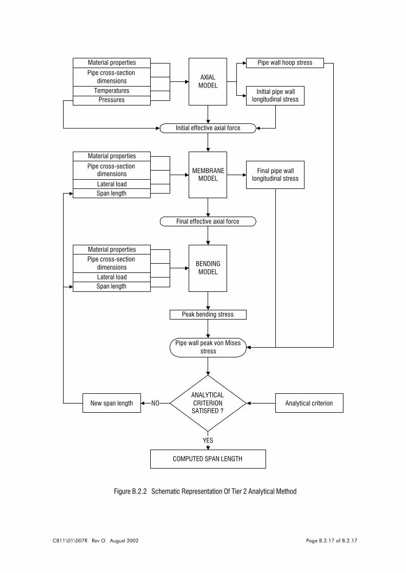
B.2.7.1 GeneralThe analytical method is shown in outline in the flow-char t given in Figure B.2.2. The purpose
of the analysis is to compute a span length for the pipe subjected to the various loadings and
an analytical criterion. The analytical method is made up of four computational modules,
namely:
! axial model (prebending state)
! membrane model
C811\01\007R Rev O August 2002 Page B.2.7 of B.2.17
! bending model
! analytical criterion.
These interact with each other within an overall framework. The framework controls the method
iteratively, changing the span length until the analytical criterion is just satisfied. The interaction
between the modules and the way the framework operates is outlined in more detail below, and
the individual models are given a fuller description in subsection B.2.7.5.
The axial model takes as inputs the pipe material proper ties and cross-section dimensions, and
internal and external temperatures and pressures. It computes, and produces as outputs, the
pipe wall hoop and longitudinal stresses, and initial effective axial force in the pipe. The latter
is aggregated from the longitudinal stress in the pipe wall times the cross-section area, and the
internal pressure times the pipe bore area. Since the computations do not involve the span
length, the axial model functions outwith the iterative loop that changes this parameter.
A cycle of iteration starts with the membrane model. This receives pipe material properties and
cross-section dimensions, lateral load, and (from the prebending model) initial effective force
as inputs. In addition to these the model uses the span length for the particular iteration cycle;
its purpose is to compute the membrane stresses that develop longitudinally in the pipe wall as
a result of sag tension, and produces as output the final effective axial force in the span.
The bending model takes pipe material properties and cross-section dimensions, lateral load,
span length, and (from the membrane model) final effective axial force. The principal output it
produces is the peak bending stress in the pipe wall.
The final stage in any cycle of iteration is the application of the analytical criterion. In this, the
pipe wall hoop stress from the axial model, the final longitudinal stresses from the membrane
model and the peak bending stress from the bending model are combined to give the peak von
Mises stress. The result is compared with the stress from the analytical criterion, and if the two
are significantly close in value, the span length is deemed to be that which is required;
otherwise, a revised span length is taken and the cycle of iteration begins again.
B.2.7.2 LoadingsThe loadings that should be applied in the analytical method are as follows:
! prestressing due to residual lay tension (to be estimated conservatively and included
if it adversely affects the pipeline)
! internal temperature q i
! internal pressure pi (which may be the normal operating, maximum allowable
C811\01\007R Rev O August 2002 Page B.2.8 of B.2.17
( )hf
f
kE
=+2 1 ν
K EA kL s h=
( )[ ]A D D ts = − −π4
22 2
l = =E A
K
E A
ks
L
s
h
operating or hydrotest pressure, whichever is under attention)
! external temperature qa
! external pressure pa (see subsection B.2.5.3, above)
! total vertical uniformly distributed load qv = q + qi (see subsections B.2.5.2 and
B.2.5.5, above)
! total horizontal uniformly distributed load qh (see subsection B.2.5.4, above).
B.2.7.3 Support ConditionsSymmetry at midspan may be assumed. In this case, appropriate symmetry boundary
conditions on displacement are enforced at midspan, and one shoulder region considered.
Regarding the shoulder region, consideration must be given to support conditions in the vertical,
transverse-horizontal and the longitudinal-horizontal directions.
For the longitudinal-horizontal direction consideration should be given to the interaction of the
extensibility of the pipeline supported at the shoulders and the deformability of the supporting
soil. It is suggested that the stiffness per unit length of the longitudinal-horizontal supporting
soil should be derived as follows:
(B.2.9)
The stiffness against longitudinal pull-in at the ends of the span is to be taken for an infinite
shoulder length and is given by:
(B.2.10)
where
(B.2.11)
The Tier 2 analytical method requires the specification of an equivalent slip length of pipe at the
shoulders, denoted as l, which gives the same stiffness against pull-in as the pipe-foundation
combination. This is given by:
(B.2.12)
As spans become larger, it is apparent that rotational bending stiffness lessens relative to the
vertical and transverse-horizontal stiffnesses of the supporting soil. In these cases, to which
the Tier 2 analytical method is most appropriate, it is in order to take fix-fix end conditions with

C811\01\007R Rev O August 2002 Page B.2.9 of B.2.17
( ) ( )σ θ = −
−p p
D t
ti a 2
( ){ }σ νσ α θ θθxos
i aNA
E= + − −
( )N A p D tao xo s i= − −σπ4
2 2
respect to rotations of the span ends about axes normal to the vertical and transverse-horizontal
planes.
B.2.7.4 Material CharacteristicThe stress-strain characteristic for the pipeline steel should be taken as elastic, with Young’s
modulus of E, Poisson’s ratio of n. Where required, the yield strength should be taken as so.
B.2.7.5 Mechanical Model
B.2.7.5.1 Axial Model
Purpose. The purpose of the axial model is to determine the longitudinal and hoop state of
stress in the pipe wall and the initial effective axial force in the pipeline.
Assumptions. The assumptions used for the axial model are as follows:
1. The structural effects of anti-corrosion and weight coats are ignored.
2. The stress-strain response of the pipe steel is elastic.
3. The pipe is fully supported along its length by the seabed, and there are no bending-
type deformations.
4. Membrane thin shell calculations based on the median sur face of the steel pipe are
sufficiently accurate for stresses, with plane stress assumptions with respect to the
through-thickness direction.
5. There is full axial restraint in the longitudinal direction, leading to thermal and Poisson-
effect stresses.
Stresses and initial effective axial force. The pipe wall stresses and initial effective axial force
are given by the following expressions:
Hoop stress σq:
(B.2.13)
Longitudinal stress σxo:
(B.2.14)
Initial effective axial force Nao:
(B.2.15)

C811\01\007R Rev O August 2002 Page B.2.10 of B.2.17
( )EI
E I s* =−1 2ν
( )[ ]I D D ts = − −π64
24 4
rI
Ass
s
=
B.2.7.5.2 Membrane Model
Purpose. The purpose of the membrane model is to determine the sag tension longitudinal
stress that develops in the pipe wall as a result of bending in the span, and the final effective
axial force.
Idealisation. The spanning portion of the problem is idealised as a planar beam with fix-fix
rotational boundary conditions. The ends of the beam are capable of translating horizontally
(“pulling-in”), but are restrained from doing so by adjoining lengths of straight pipe (“slip
lengths”) on the shoulders that are anchored at their ends remote from the spanning portion.
The whole of the model (span plus the two slip lengths) are initially subject to an effective axial
force; the span portion is also loaded by a uniformly distributed lateral load.
Assumptions. The assumptions used for the membrane model are as follows:
1. Only longitudinal stresses may occur in the pipe wall within the slip length.
2. There are no rotations at the ends of the freespan portion of the model.
3. There is compatibility of longitudinal displacement at the junctions between the
spanning and slip length portions of the model.
4. The stress-strain response of the pipe steel is elastic.
5. The initial effective axial force is uniform along the length of the model.
6. The membrane tension developed in response to the bending is uniform along the
length of the model.
7. Euler-Bernoulli beam-bending theory applies to the spanning portion of the model.
Parameters. The parameters are derived using baseline data and other expressions derived in
subsection 2.7.5.1, above, as follows:
Equivalent bending rigidity of the pipe EI*:
(B.2.16)
where
(B.2.17)
Pipe cross-section radius of gyration rs:
(B.2.18)
C811\01\007R Rev O August 2002 Page B.2.11 of B.2.17
q q qn v h= +2 2
λπ
=
14
14q r
E ALr
n s
s s
nN
EI
EI rqao
ao s
n
= *
*
4
( )ζ λ ζ λ ζ− +
++ =4 3 2
16 20
LL
n aol
ζδ
=m
sr
( )u
L L m=+
π δ2 2
4 2l
l
( )n
LLa =
+4 22
lζ
N N EIL
na ao a= +
* π 2
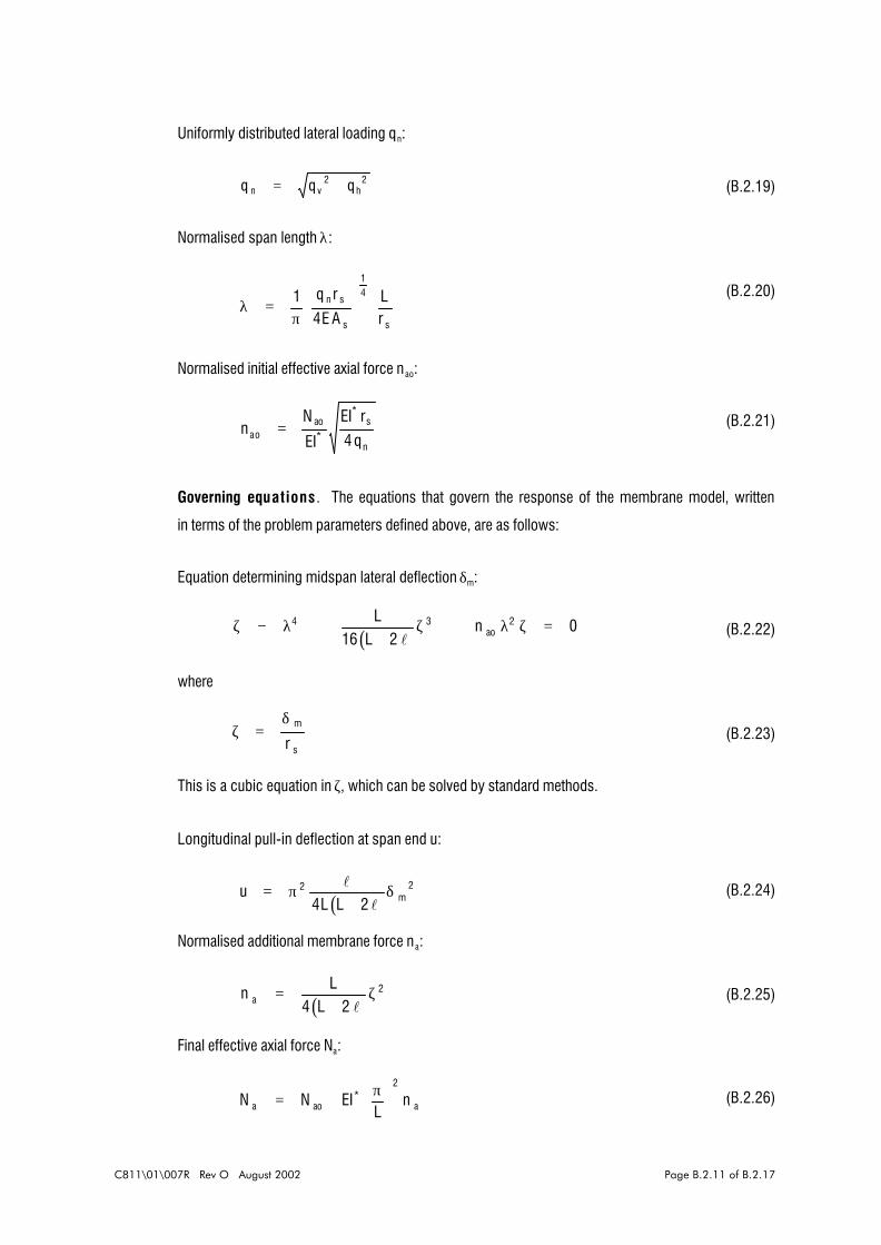
Uniformly distributed lateral loading qn:
(B.2.19)
Normalised span length λ:
(B.2.20)
Normalised initial effective axial force nao:
(B.2.21)
Governing equations . The equations that govern the response of the membrane model, written
in terms of the problem parameters defined above, are as follows:
Equation determining midspan lateral deflection δm:
(B.2.22)
where
(B.2.23)
This is a cubic equation in ζ, which can be solved by standard methods.
Longitudinal pull-in deflection at span end u:
(B.2.24)
Normalised additional membrane force na:
(B.2.25)
Final effective axial force Na:
(B.2.26)

C811\01\007R Rev O August 2002 Page B.2.12 of B.2.17
σ σπ
xa xos
aEIA L
n= +
* 2
σθ θθ θ
σθ θ
θ θ
xbs
na
xbs
na
DI
q Lif N
DI
q Lif N
=−
≥
=−
<
2 40
2 40
2
2
2
2
tanhtanh
tantan
θ =L N
EIa
2 *
Final pipe wall longitudinal stress σxa:
(B.2.27)
B.2.7.5.3 Bending ModelPurpose. The purpose of the bending model is to determine the peak longitudinal bending stress
in the pipe wall when the span is loaded by the uniformly distributed lateral load and the final
effective axial force.
Idealisation. The span portion only is considered. This is treated as a beam with fix-fix end
conditions under uniformly distributed lateral load and an axial force.
Assumptions. The assumptions used in the bending model are as follows:
1. There is no rotation at the ends of the span.
2. There is no restraint against pull-in at the ends of the span.
3. The stress-strain response of the pipe steel is elastic.
4. Small deflection theory applies.
5. Euler-Bernoulli beam-bending theory applies.
Governing equations. The equations that govern the response of the bending model, written in
terms of the problem parameters defined above, are as follows:
Peak bending stress σxb:
(B.2.28)
where
(B.2.29)

C811\01\007R Rev O August 2002 Page B.2.13 of B.2.17
δθ
θ θ
δθ
θ θ
bn
a
bn
a
q L
EIif N
q L
EIif N
= −
≥
=
−
<
4
3
4
3
161
2 20
161
2 20
*
*
tanh
tan
( ) ( )
( ) ( )
MAX OR
xa b xa b
xa b xa b
o
σ σ σ σ σ σ
σ σ σ σ σ σ
σ ξ
θ θ
θ θ
+ − + +
− − − +
− ≤
2 2
2 2
L Lobs comp≤ 0 9.
Midspan lateral deflection δb:
(B.2.30)
B.2.7.5.4 Use Of Analytical Criterion
The span length is deemed to have reached the magnitude necessary to satisfy the analytical
criterion when the following condition is satisfied:
(B.2.31)
where σo is the percentage of SMYS determined using the analytical criterion as set out in
subsection B.2.6.2, and ξ is a convergence tolerance close to zero.
B.2.7.6 Analytical Method ImplementationThe analytical method has been implemented into a spreadsheet program. An example of an
analysis proforma is given in Section B.3, ATTACHMENTS.
B.2.8 ACCEPTANCE CRITERION
The output from the Tier 2 static strength analysis method is a computed span length Lcomp. A
percentage of this is compared with the observed span length to determine acceptability of the
latter; the percentage suggested is 90%. Hence, the criterion for acceptability of the observed
span is:
(B.2.32)

C811\01\007R Rev O August 2002 Page B.2.14 of B.2.17
Data Symbol
Pipeline DataPipe outside diameter D
Pipe nominal wall thickness t
Corrosion coat thickness teWeight coat thickness tcSteel density ρs
Corrosion coat density ρe
Weight coat density ρc
Steel elastic modulus E
Steel Poisson’s ratio ν
SMYS steel σy
Steel thermal expansion coefficient α
Axial restraint factor λa
Pipeline heading ϕ
Operational Data
Residual lay tension NInternal pressure pi
Contents density ρi
Contents temperature θi
Design life of pipeline Tp
Environmental Data
Minimum water depth at LAT h
Local seawater density ρa
Local seawater temperature θa
Current velocity data -
Wave data -
Hydrodynamic drag coefficient Cd
Hydrodynamic added mass coefficient Ca
Soil elastic modulus at span shoulders Ef
Soil Poisson’s ratio at span shoulders νf
Longitudinal friction coefficient at span shoulders µL
Transverse friction coefficient at span shoulders µT
Inspection Data
Kilometre point at start of span KPs
Kilometre point at end of span KPe
Freespan length Lobs
Gap beneath span G
Marine growth information -
Table B.2.1 Data Classes
C811\01\007R Rev O August 2002 Page B.2.15 of B.2.17
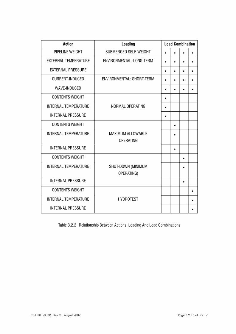
Action Loading Load Combination
PIPELINE WEIGHT SUBMERGED SELF-WEIGHT • • • •EXTERNAL TEMPERATURE ENVIRONMENTAL: LONG-TERM • • • •
EXTERNAL PRESSURE • • • •CURRENT-INDUCED ENVIRONMENTAL: SHORT-TERM • • • •
WAVE-INDUCED • • • •CONTENTS WEIGHT •
INTERNAL TEMPERATURE NORMAL OPERATING •INTERNAL PRESSURE •CONTENTS WEIGHT •
INTERNAL TEMPERATURE MAXIMUM ALLOWABLE
OPERATING•
INTERNAL PRESSURE •CONTENTS WEIGHT •
INTERNAL TEMPERATURE SHUT-DOWN (MINIMUM
OPERATING)•
INTERNAL PRESSURE •CONTENTS WEIGHT •
INTERNAL TEMPERATURE HYDROTEST •INTERNAL PRESSURE •
Table B.2.2 Relationship Between Actions, Loading And Load Combinations

C811\01\007R Rev O August 2002 Page B.2.16 of B.2.17
ACCEPT SPAN?
DATA
ANALYTICAL CRITERIA
LOAD COMBINATION
APPLY TIER 1 STATIC STRENGTHANALYTICAL METHOD
COMPUTED SPAN LENGTH
OBSERVED SPAN LENGTH
YES
NO
ACCEPT SPAN?
APPLY TIER 2 STATIC STRENGTHANALYTICAL METHOD
COMPUTED SPAN LENGTH
YES
NO
ACCEPTANCE CRITERION
ACCEPT SPAN?
APPLY TIER 3 STATIC STRENGTHANALYTICAL METHOD
COMPUTED STRESS, STRAINOVALISATION
YES
NO
START OF DYNAMICSTRENGTH ASSESSMENT
CLASSIFY AS SIGNIFICANT
DATA
ACCEPTANCE CRITERIA:STRESSSTRAIN
OVALISATION
DATA
ANALYTICAL CRITERIA
ACCEPTANCE CRITERION
RECTIFY SPAN
START OF STATICSTRENGTH ASSESSMENT
OBSERVED SPAN LENGTH
OBSERVED SPAN LENGTH
Figure B.2.1 Static Strength Assessment At The Tier 2 Level
C811\01\007R Rev O August 2002 Page B.2.17 of B.2.17
AXIALMODEL
MEMBRANEMODEL
BENDINGMODEL
ANALYTICALCRITERIONSATISFIED ?
Pipe wall peak von Misesstress
COMPUTED SPAN LENGTH
YES
Final effective axial force
Initial effective axial force
New span length NO
Material properties
TemperaturesPressures
Span length
Pipe cross-sectiondimensions
Lateral load
Material properties
Material propertiesPipe cross-section
dimensionsLateral loadSpan length
Pipe wall hoop stress
Initial pipe walllongitudinal stress
Peak bending stress
Pipe cross-sectiondimensions
Final pipe walllongitudinal stress
Analytical criterion
Figure B.2.2 Schematic Representation Of Tier 2 Analytical Method

C811\01\007R Rev O August 2002 Page B.3.1 of B.3.1
TIER 2 Membrane effects STATIC STRENGTH span assessment methodPipeline data- Symbol Value (Units)Pipeline segment identification ID PL-774-GKilometre start point KPs 397 kmKilometre end point KPe 404.4 kmOutside diameter D 914.4 mmNominal wall thickness t 28.4 mmCorrosion coat thickness te 6 mmWeight coat thickness tc 76 mmSteel density rs 7850 kg/m^3Corrosion coat density re 1400 kg/m^3Weight coat density rc 3040 kg/m^3Steel elastic modulus E 207000 N/mm^2Steel Poissons ratio nu 0.3Steel SMYS SMYS 448.3 N/mm^2Steel coeff. of thermal expansion alf 0.0000116 ° C^-1
Operational conditions data- (Units)Residual lay tension Nlay 0 NContents pressure pnorm 10 N/mm^2Contents density ri 105.4 kg/m^3Contents temperature thi 10 ° C
Environmental data- (Units)Gravitational acceleration g 9.81 m/s^2Minimum water depth at LAT h 45 mCurrent speed at top of pipe Vc 0.51 m/sMax. wave induced velocity at top of pipe Vw 0.95 m/sLocal seawater density rw 1025 kg/m^3Local seawater temperature tha 4 ° CHydrodynamic drag coefficient Cd 1.05Pipeline longitudinal slip length Lslip 50 m
Safety factors- (Units)Safety factor on span lls 0.9Factor on SMYS Ksmys1 0.96P-delta effect switch (0 = off, 1 = on) SWPD 1Membrane effect switch (0 = off, 1 = on) SWMB 1Convergence norm for solution routine CONV 0.001
Principal results-Submerged weight of pipe/unit length q 4876.35 N/mHorizontal loading/unit length qh 1237.00 N/mMaximum loading/unit length qmx 5030.80 N/mHoop stress Sh 148.93 N/mm^2Net prebending longitudinal stress 30.27 N/mm^2Additional membrane stress 75.88 N/mm^2Bending stress 378.90 N/mm^2Peak equivalent stress 430.37 N/mm^2Initial membrane axial force 2.39E+06 NBore pressure axial force -5.78E+06 NInitial effective axial force -3.38E+06 NAdditional effective axial force 6.00E+06 NFinal effective axial force 2.61E+06 NMidspan lateral deflection (from bending) 2.0343 mMidspan lateral deflection (from membrane) 2.2451 mEnd pull-in (at one end) 0.0167 mError check on span length calculation OK
Factored allowable span length Ls2 134.5 m
B.3 ATTACHMENTS
Table B.3.1 Example of Tier 2 Static Strength Analysis Proforma
C811\01\007R Rev O August 2002 Page C.0.1 of C.0.4
APPENDIX C
PIPELINE DEFECT A SSESSMENT
PROCESS: SPAN ANALYSIS FOR
STATIC STRENGTH AT THE TIER 3
LEVEL

C811\01\007R Rev O August 2002 Page C.0.2 of C.0.4
TABLE OF CONTENTS
Page No
C.1
C.2
INTRODUCTION
C.1.1 PURPOSE
C.1.2 SCOPE AND LIMITATIONS
C.1.3 REFERENCES
C.1.3.1 Codes And Standards
PROCESS
C.2.1 OBJECTIVE
C.2.2 ASSESSMENT STRATEGY AT THE TIER 3 LEVEL
C.2.2.1 Generic
C.2.2.2 Considerations In The Tier 3 Static Strength Analytical Method
C.2.3 DATA
C.2.3.1 Data Classes
C.2.3.2 Data Sources
C.2.4 LOADINGS AND LOAD COMBINATIONS IN GENERAL
C.2.4.1 General Points
C.2.4.2 Actions
C.2.4.3 Loadings
C.2.5 LOAD COMBINATION IN FINITE ELEMENT ANALYSIS
C.2.5.1 Load Combination
C.2.5.2 Submerged Self-Weight
C.2.5.3 Environmental: Long-Term
C.2.5.4 Environmental: Short-Term
C.2.5.5 Operating
C.2.6 TIER 3 (FINITE ELEMENT) STATIC STRENGTH ANALYTICAL METHOD
C.2.6.1 Finite Element Package
C.2.6.2 Loadings
C.2.6.3 Element Types
C.2.6.4 Element Mesh
C.2.6.5 Support Conditions
C.2.6.6 Material Characteristic
C.2.6.7 Analysis Options
C.2.6.8 Analysis Procedure
C.1.1
C.1.1
C.1.1
C.1.1
C.1.1
C.2.1
C.2.1
C.2.1
C.2.1
C.2.1
C.2.2
C.2.2
C.2.2
C.2.3
C.2.3
C.2.3
C.2.3
C.2.4
C.2.4
C.2.4
C.2.4
C.2.5
C.2.5
C.2.5
C.2.5
C.2.6
C.2.6
C.2.7
C.2.7
C.2.9
C.2.9
C.2.9

C811\01\007R Rev O August 2002 Page C.0.3 of C.0.4
TABLE OF CONTENTS/continued
C.2.7 ACCEPTANCE CRITERIA C.2.9
C.2.7.1 General C.2.9
C.2.7.2 Stress Criterion C.2.9
C.2.7.3 Strain Criterion C.2.9
C.2.7.4 Ovalisation Criterion C.2.11
C.2.7.5 Local Buckling Criterion C.2.11
C.3 ATTACHMENTS C.3.1
C811\01\007R Rev O August 2002 Page C.0.4 of C.0.4
LIST OF TABLES
Table C.2.1 Data Classes
Table C.2.5 Relationship Between Actions, Loading And Load Combinations
LIST OF FIGURES
Figure C.2.1 Static Strength Assessment At The Tier 3 Level

C811\01\007R Rev O August 2002 Page C.1.1 of C.1.1
C.1 INTRODUCTION
C.1.1 PURPOSE
The purpose of this process document is to set down the considerations for the finite element
static strength analysis of pipeline spans at the Tier 3 level and to ensure that best practice is
applied.
C.1.2 SCOPE AND LIMITATIONS
This process applies to pipelines laid directly onto the seabed. It applies to an individual span;
that is, a single clear unsupported length of pipeline that is sufficiently isolated from other spans
or features as to be judged to behave as a self-contained entity. It does not apply to pipelines
that are trenched, trenched and backfilled, trenched and infilled due to natural soil migration, or
pipelines that are piggybacked.
C.1.3 REFERENCES
C.1.3.1 Codes And Standards! Rules For Submarine Pipeline Systems. Det Norske Veritas. DNV, 1996.
! Code Of Practice For Pipeline Subsea: Design, Construction And Installation. British
Standards Institute (BSI). BS 8010: Part 3: 1993.
! American Petroleum Institute (API). Recommended Practice For Planning, Designing,
And Constructing Fixed Offshore Platforms - Working Stress Design. RP2A-WSD,
20th ed., July 1993.

C811\01\007R Rev O August 2002 Page C.2.1 of C.2.14
C.2 PROCESS
C.2.1 OBJECTIVE
The objective of this process document is to ensure that the finite element analysis of pipeline
spans is conducted in a rigorous manner, with due regard to the mechanical characteristics of
the problem, and that spans are determined to be acceptable or significant against acceptance
criteria.
C.2.2 ASSESSMENT STRATEGY AT THE TIER 3 LEVEL
C.2.2.1 GenericThe recommended Pipeline Defect Assessment Procedure allows a tiered approach to analytical
methods and span acceptance. Specifically, up to a three-tiered philosophy can be adopted
as shown in detail for the failure mode of static strength in Figure 2.1. In this figure, the lower
level tiers have been greyed, leaving the Tier 3 assessment covered by this process highlighted.
At whatever tier level, the approach involves interaction between the data, load combinations,
analytical criteria, analytical methods and acceptance criteria; with the exception of analytical
criteria, each of these is dealt with in detail in subsections 2.3 to 2.7, below. At Tier 3,
observed span lengths are analysed with the results judged against acceptance criteria to
determine acceptability:
! observed span length forms part of the input to the analytical method
! analytical criteria in the lower tiers are acceptance criteria at the Tier 3 level
! the output from the Tier 3 analytical method relates directly to the acceptance criteria
employed.
C.2.2.2 Considerations In The Tier 3 Static Strength Analytical MethodIn using finite element methods for the analysis of pipeline spans consideration should be given
to the following factors:
! finite element package
! loadings
! element types
! element mesh
! support conditions

C811\01\007R Rev O August 2002 Page C.2.2 of C.2.14
! material characteristic
! analysis options
! analysis procedure.
Each of these points is addressed in detail in subsection C.2.6, below.
C.2.3 DATA
C.2.3.1 Data ClassesA detailed breakdown of the data into the four classes of: pipeline, operational, environmental
and inspection is given in Table C.2.1. Data in the lines of Table C.2.1 that have been greyed
are considered to be unnecessary to perform the static strength finite element analysis. The
remainder can be viewed as “baseline” data, some of which has to be processed by means of
calculation into suitable input data for the finite element analysis.
The pipeline data include geometrical and material proper ties; these are used to construct the
finite element model and its material characteristic.
The operational data encompass installation (residual lay tension) and those related to the pipe
contents: its density, pressure and temperature; these are used to derive some of the loadings
applied to the span.
The environmental data include the parameters that relate to the fluid loading on the pipeline
(for example, water depth and various wave and current data). They also contain parameters
defining the mechanical interaction between the pipe and the seabed (for example, soil modulus
and Poisson’s ratio at the span shoulders, and longitudinal and transverse coefficients of friction
between the pipeline and the seabed); these particular parameters influence the support
conditions at the shoulder of the pipeline.
The inspection data include parameters to locate the span (kilometre start and end points), and
freespan length. If marine growth information is included within the inspection data an
assessment should be made as to whether this influences the pipeline weight or the
hydrodynamic loading on the pipeline.
C.2.3.2 Data SourcesAppropriate sources of pipeline, operational and environmental data are to be used. If no data
are available for residual lay tension, then it is to be estimated conservatively and included i f
it adversely affects the pipeline.

C811\01\007R Rev O August 2002 Page C.2.3 of C.2.14
C.2.4 LOADINGS AND LOAD COMBINATIONS IN GENERAL
C.2.4.1 General PointsA load combination is built up from actions and loadings as shown schematically in Table C.2.2.
The loading combination to be used is a requirement of the assessment, and as indicated in
subsection C.2.5 an operating loading is always included in the combination. This will usually
correspond to the normal operating conditions of the pipeline, although there may be occasions
where other operating conditions need to be considered.
C.2.4.2 ActionsIn terms of detailed thermo-mechanical actions there are eight types that require consideration:
! pipeline weight
! external temperature
! external pressure
! current-induced action
! wave-induced action
! contents weight
! internal temperature
! internal pressure.
C.2.4.3 LoadingsFour individual loading classes are to be considered, namely:
! submerged self weight
! environmental: long-term
! environmental: short-term
! operating.
More than one type of operating condition may need to be addressed. As indicated in Table 2.5,
the list covers the following possibilities:
! normal operating
! maximum allowable operating
! shut down (minimum operating)
! hydrotest.
This list may be extended if circumstances dictate.

C811\01\007R Rev O August 2002 Page C.2.4 of C.2.14
q q q q qs e c a= + + −
( )[ ]ssq
gD D t= − −
ρ π
422 2
( )ee
eqg
D t D= + −
ρ π
42
2 2
( ) ( )cc
e c eqg
D t t D t= + + − +
ρ π
42 2 2
2 2
( )aa
e cqg
D t t= + +ρ π
42 2
2
a ap gh= ρ
C.2.5 LOAD COMBINATION IN FINITE ELEMENT ANALYSIS
C.2.5.1 Load CombinationA load combination is made up from loading classes, and will always comprise the submerged
self-weight, environmental long- and shor t-term load and an operating class, as set out
schematically in Table C.2.2.
C.2.5.2 Submerged Self-WeightThe submerged self-weight should comprise the weight of the pipe, anti-corrosion coating and
weight coating, minus the displaced weight of seawater. It is calculated from the data as
follows:
(C.2.1)
(C.2.2)
(C.2.3)
(C.2.4)
(C.2.5)
The symbols are explained in Table C.2.1.
The submerged self-weight may be augmented by an estimate of additional gravity load due to
marine fouling, if appropriate.
C.2.5.3 Environmental: Long-TermThe only part of the environmental: long-term loading that requires derivation is the external
(hydrostatic) pressure. This may be estimated from:
(C.2.6)
C811\01\007R Rev O August 2002 Page C.2.5 of C.2.14
( )( )h a d e c c wq C D t t V V= + + +12
2 22
ρ
( )iiq
gD t= −
ρ π
42 2
C.2.5.4 Environmental: Short-TermThe environmental: short-term loading comprises the hydrodynamic uniformly distributed load
resulting from the drag on the pipeline from the moving water particle velocities. Inertia loading
is generally small, and in most circumstances may be neglected. It is recommended that
directional 50-year return period maximum wave height and period (Hmax and Tmax), and
associated maximum surface current velocity are used to determine the maximum combined
water particle velocity normal to the heading of the span, which forms the input to Morison’s
equation to derive the loading on the span. The main steps in this process are as follows:
1. Use directional 50-year return period maximum wave height and period (Hmax and
Tmax), and associated maximum surface current velocity
2. Considering the heading of the pipeline span, determine the maximum wave height
and corresponding period, and associated surface current velocity normal to the
pipeline span
3. Compute the top-of-pipe current velocity Vc using a power-law current profile
suggested in the source data
4. Compute the top-of-pipe maximum wave velocity Vw using a wave theory suitable for
the Hmax - Tmax - water depth combination concerned (kinematic spreading may be
neglected, and the effect of current velocity on wave period may be ignored)
5. The uniformly distributed load is then derived from:
(C.2.7)
The environmental: short-term loading may be augmented by an estimate of additional load due
to marine fouling, if appropriate.
C.2.5.5 OperatingThe only part of the operating loading that requires derivation is the contents self-weight. This
is given by:
(C.2.8)
C.2.6 TIER 3 (FINITE ELEMENT) STATIC STRENGTH analytical method
C.2.6.1 Finite Element PackageA reputable, well-validated package should be used to conduct the finite element analysis of
spans. The principal requirements of the package are that it has an appropriate range of

C811\01\007R Rev O August 2002 Page C.2.6 of C.2.14
elements, has non-linear capabilities (both geometric and material) and has facilities for
applying the types of loadings required.
C.2.6.2 LoadingsThe loadings that should be applied to the finite element model should be as follows:
! prestressing due to residual lay tension (to be estimated conservatively and included
if it adversely affects the pipeline)
! internal temperature θi
! internal pressure pi (which may be the normal operating, maximum allowable
operating or hydrotest pressure, whichever is under attention; consideration should
also be given to omitting the internal pressure if this is appropriate to the acceptance
criterion under use, see subsection C.2.7)
! external temperature θa
! external pressure pa (see subsection C.2.5.3, above)
! total vertical uniformly distributed load qv = q + qi (see subsections C.2.5.2 and
C.2.5.5, above)
! total horizontal uniformly distributed load qh (see subsection C.2.5.4, above).
C.2.6.3 Element TypesElements are required in order to model the pipeline and the seabed.
In general, codes do not allow the weight coat to be considered to contribute str ucturally to the
pipeline (see, BS 8010: Part 3: 1993 and DNV, 1996) and so elements are only required to
model the steel pipe. These should have the following capabilities:
! three-dimensional beam action
! P - δ effects
! hoop stress and strain, as well as longitudinal stress and strain
! temperature and pressure effects
! end-cap effects, if necessary
! section deformation (if an acceptance criterion involving ovalisation is being used; see
subsection C.2.7.4 below).
In using tailor-made elements, such as PIPE or ELBOW-type elements in ABAQUS for example,
consideration should be given to any diameter to thickness limitations inherent in the element
formulations.
Possible options for elements used to represent the seabed may be extension/compression
C811\01\007R Rev O August 2002 Page C.2.7 of C.2.14
springs, or rigid-surface. In the case of springs, the principal requirement is that they allow a
non-linear load-deflection response to be specified. The requirements for rigid-surface elements
are that they allow contact with the pipe elements and hence upl i f t, and that they have the
capability of modelling friction between the surface and the pipe elements.
C.2.6.4 Element MeshIn meshing the finite element model two distinct regions need to be considered: the span region
and the shoulder region. Providing that conditions at the two shoulders of the span can be
considered to be identical, then symmetry at midspan may be assumed and a half-model built;
this will comprise half the span length (as dictated by the value observed in the inspection, Lobs)
coupled to one shoulder-supported region.
Generally, in the span region, elements to represent the pipe will only be required. A suitably
graded mesh for these elements must be used that has regard for the generation of peak
bending moments at midspan and around the junction between the span and the shoulder, and
the possibility of bar buckling. Aspect ratio (length to diameter) restrictions of the elements are
not to be violated in generating the mesh.
In the shoulder region(s) elements will be required to represent both the pipe and the seabed.
As such, a number of factors require careful consideration:
! the length of the pipe part of the finite element model should be such as to represent
semi-infinite conditions
! the density and node spacing of elements used to represent the pipe must have
regard for the generation of peak bending moment around the junction between the
span and the shoulder, and aspect ratio (length to diameter) restrictions of the
elements
! the spacing of discrete springs, which may be used to represent the seabed (see
subsection C.2.6.5, below), must be such as to replicate continuous support
! the extent of rigid surfaces, which may be used to represent the seabed (see
subsection C.2.6.5, below), must be such as to represent semi-infinite conditions.
C.6.5 Support ConditionsThe support conditions to be enforced depend on whether or not symmetry at midspan of the
model has been assumed (see subsection 2.6.4, above). If a full model is to be used then
considerations of suppor t conditions are confined to the two shoulder regions. In the event that

C811\01\007R Rev O August 2002 Page C.2.8 of C.2.14
( )vf
f
kE
=−2 1 2ν
( )hf
f
kE
=+2 1 ν
LL L vf q= µ
LT T vf q= µ
a half-model is used, then appropriate symmetry boundary conditions on displacement must
be enforced at midspan, and one shoulder region considered.
Regarding the shoulder regions, consideration must be given to support conditions in the
vertical, transverse-horizontal and longitudinal-horizontal directions. The use of two main types
of support to replicate the pipeline/seabed interaction at the span shoulder is suggested:
1. continuous elastic foundation (or discrete elastic springs) in the vertical plane to
model deformability of the seabed; and discrete elastic-perfectly plastic springs in the
transverse and longitudinal horizontal directions to model deformability and frictional
slip
3. rigid-sur face with friction interaction between pipe elements and the surface to
provide: restraint in the vertical, and both horizontal directions; and the facility for lif t-
off of the pipeline from the rigid surface at the shoulders.
For elastic constants to be used in support type 1, above, it suggested that the stiffness per unit
length of the vertical support should be derived as follows:
(C.2.9)
and the stiffness per unit length of the transverse and longitudinal support should be derived as
follows:
(C.2.10)
The limiting force per unit length of the longitudinal and transverse springs should be determined
from:
(C.2.11)
(C.2.12)
respectively.
In view of the fact that discrete springs may be used for the vertical, longitudinal- and
transverse-horizontal directions, then the stiffness and limiting forces for these springs should
be obtained by multiplying the above values by the longitudinal spacing of the springs in the
finite element model.
C811\01\007R Rev O August 2002 Page C.2.9 of C.2.14
The rigid surface support (type 2, above) requires only the specification of the friction
coefficients in the longitudinal and transverse horizontal directions. Appropriate values of mL and
mT are to be taken.
C.2.6.6 Material CharacteristicThe stress-strain characteristic for the pipeline steel should be taken as elastic-perfectly plastic.
Care must be taken, however, in that some finite element packages require tr ue (rather than
engineering) parameters to be specified.
C.2.6.7 Analysis OptionsThe analysis options should include full geometric and material non-linearity. Consideration
should be given to the use of displacement control, the Riks method, or other non-linear solution
procedures if necessary.
C.2.6.8 Analysis ProcedureThe analysis procedure to be used depends on the finite element package. Given that material
non-linearity may occur in the analysis, it is important to appreciate that if plasticity develops,
then the order of load application may affect results. This is a par ticular consideration if an
acceptance criterion involving plastic strain is adopted (see subsection 2.7.3, below). In the
light of this, careful consideration needs to be given to the order of load application as it relates
to the formation of the span.
Thus in the case of a span formed by soil migration from beneath the pipeline, it may be judged
appropriate to apply the internal and external temperatures and pressures, plus the total vertical
uniformly distributed load in a single load-step, followed by the total horizontal uniformly
distributed load as a separate load-step (this has the effect of separating out the environmental:
short-term loading effects from the spanning effects). Another possibility is to apply all loading
to the shoulder por tion of the model as a first load-step, followed by all the loading on the
freespan por tion of the model as a second load-step (this has the effect of separating out the
as-laid and span formation aspects of the problem).
C.2.7 ACCEPTANCE CRITERIA
C.2.7.1 GeneralThere is a general requirement that the analytical outputs must have the capacity for ready
comparison with the acceptance criteria. Precisely how this is handled depends on the exact
details of the FEA model employed in the analytical method. It is worth noting that, for example,
if the type of elements used in the FE representation are such that ovalisation and local buckling
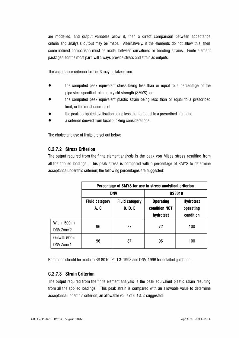
C811\01\007R Rev O August 2002 Page C.2.10 of C.2.14
are modelled, and output variables allow it, then a direct comparison between acceptance
criteria and analysis output may be made. Alternatively, if the elements do not allow this, then
some indirect comparison must be made, between curvatures or bending strains. Finite element
packages, for the most part, will always provide stress and strain as outputs.
The acceptance criterion for Tier 3 may be taken from:
! the computed peak equivalent stress being less than or equal to a percentage of the
pipe steel specified minimum yield strength (SMYS); or
! the computed peak equivalent plastic strain being less than or equal to a prescribed
limit; or the most onerous of
! the peak computed ovalisation being less than or equal to a prescribed limit; and
! a criterion derived from local buckling considerations.
The choice and use of limits are set out below.
C.2.7.2 Stress CriterionThe output required from the finite element analysis is the peak von Mises stress resulting from
all the applied loadings. This peak stress is compared with a percentage of SMYS to determine
acceptance under this criterion; the following percentages are suggested:
Percentage of SMYS for use in stress analytical criterion
DNV BS8010
Fluid category
A, C
Fluid category
B, D, E
Operating
condition NOT
hydrotest
Hydrotest
operating
condition
Within 500 m
DNV Zone 296 77 72 100
Outwith 500 m
DNV Zone 196 87 96 100
Reference should be made to BS 8010: Part 3: 1993 and DNV, 1996 for detailed guidance.
C.2.7.3 Strain CriterionThe output required from the finite element analysis is the peak equivalent plastic strain resulting
from all the applied loadings. This peak strain is compared with an allowable value to determine
acceptance under this criterion; an allowable value of 0.1% is suggested.

C811\01\007R Rev O August 2002 Page C.2.11 of C.2.14
( )max min .5%D D
DOOR
−≤ −
21
C.2.7.4 Ovalisation CriterionThe output required from the finite element analysis is the peak cross-section ovalisation
resulting from the applied loadings. This peak ovalisation is compared with an allowable value
to determine acceptance under this criterion. It is suggested that an allowable value of 1.5%,
corrected for the out-of-roundness (OOR) tolerance from fabrication of the pipe, is used giving
a criterion as follows:
(C.2.13)
where Dmax and Dmin are the maximum and minimum diameters, respectively, on the most highly
ovalised cross-section.
Given that internal pressure has an ameliorating effect on ovalisation, consideration should be
given to a load combination that excludes internal pressure.
C.2.7.5 Local Buckling CriterionThis is related to the collapse of the cross-section section. If the finite element model allows
it, then this phenomenon can be directly monitored and the acceptance criterion becomes one
of determining if there is an adequate margin against local buckling under the applied loadings.
Given that internal pressure has an ameliorating effect on local buckling, consideration should
be given to a load combination that excludes internal pressure.
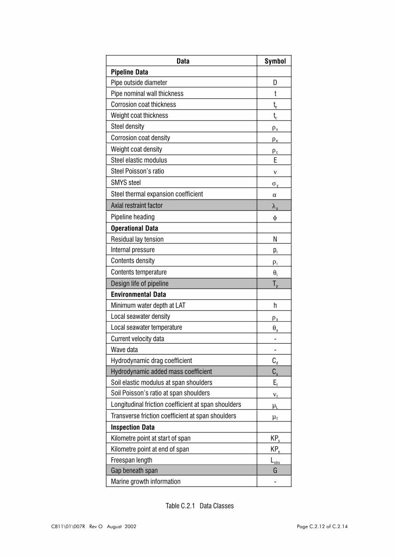
C811\01\007R Rev O August 2002 Page C.2.12 of C.2.14
Data Symbol
Pipeline DataPipe outside diameter D
Pipe nominal wall thickness t
Corrosion coat thickness teWeight coat thickness tcSteel density ρs
Corrosion coat density ρe
Weight coat density ρc
Steel elastic modulus E
Steel Poisson’s ratio ν
SMYS steel σy
Steel thermal expansion coefficient α
Axial restraint factor λa
Pipeline heading ϕ
Operational Data
Residual lay tension NInternal pressure pi
Contents density ρi
Contents temperature θi
Design life of pipeline Tp
Environmental Data
Minimum water depth at LAT h
Local seawater density ρa
Local seawater temperature θa
Current velocity data -
Wave data -
Hydrodynamic drag coefficient Cd
Hydrodynamic added mass coefficient Ca
Soil elastic modulus at span shoulders Ef
Soil Poisson’s ratio at span shoulders νf
Longitudinal friction coefficient at span shoulders µL
Transverse friction coefficient at span shoulders µT
Inspection Data
Kilometre point at start of span KPs
Kilometre point at end of span KPe
Freespan length Lobs
Gap beneath span G
Marine growth information -
Table C.2.1 Data Classes

C811\01\007R Rev O August 2002 Page C.2.13 of C.2.14
Action Loading Load Combination
PIPELINE WEIGHT SUBMERGED SELF-WEIGHT • • • •EXTERNAL TEMPERATURE ENVIRONMENTAL: LONG-TERM • • • •
EXTERNAL PRESSURE • • • •CURRENT-INDUCED ENVIRONMENTAL: SHORT-TERM • • • •
WAVE-INDUCED • • • •CONTENTS WEIGHT •
INTERNAL TEMPERATURE NORMAL OPERATING •INTERNAL PRESSURE •CONTENTS WEIGHT •
INTERNAL TEMPERATURE MAXIMUM ALLOWABLE
OPERATING•
INTERNAL PRESSURE •CONTENTS WEIGHT •
INTERNAL TEMPERATURE SHUT-DOWN (MINIMUM
OPERATING)•
INTERNAL PRESSURE •CONTENTS WEIGHT •
INTERNAL TEMPERATURE HYDROTEST •INTERNAL PRESSURE •
Table C.2.2 Relationship Between Actions, Loading And Load Combinations
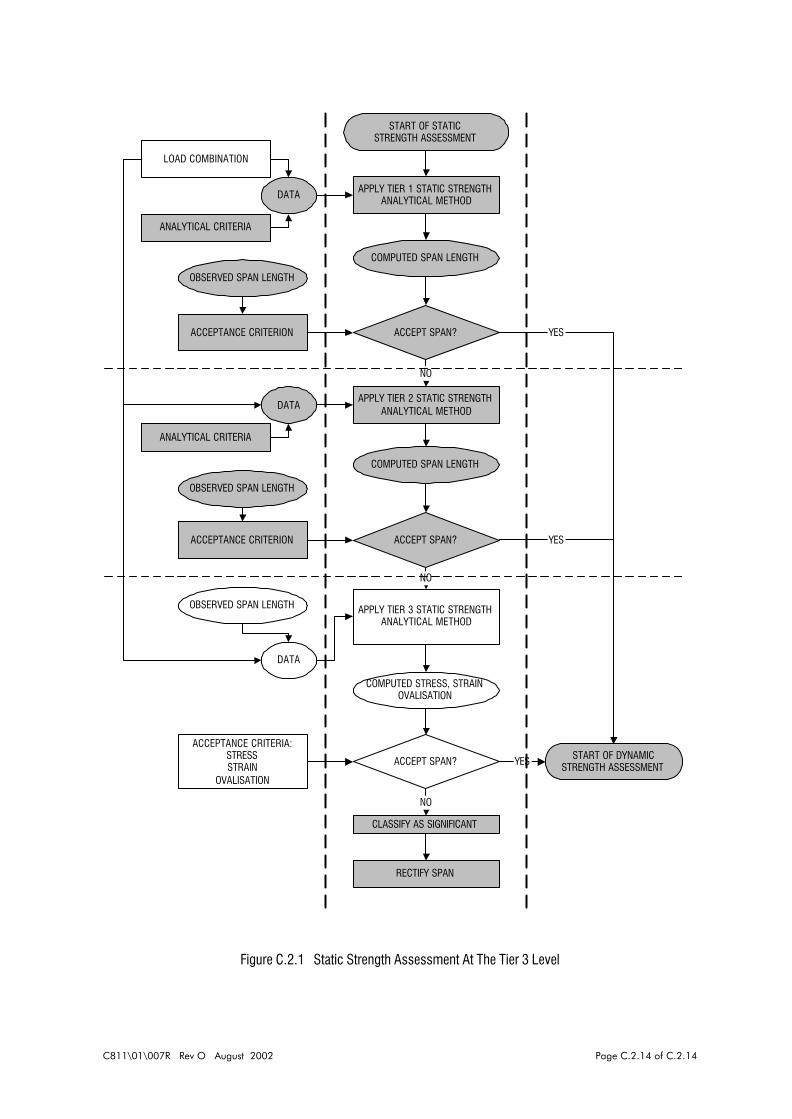
C811\01\007R Rev O August 2002 Page C.2.14 of C.2.14
ACCEPT SPAN?
DATA
ANALYTICAL CRITERIA
LOAD COMBINATION
APPLY TIER 1 STATIC STRENGTHANALYTICAL METHOD
COMPUTED SPAN LENGTH
OBSERVED SPAN LENGTH
YES
NO
ACCEPT SPAN?
APPLY TIER 2 STATIC STRENGTHANALYTICAL METHOD
COMPUTED SPAN LENGTH
YES
NO
ACCEPTANCE CRITERION
ACCEPT SPAN?
APPLY TIER 3 STATIC STRENGTHANALYTICAL METHOD
COMPUTED STRESS, STRAINOVALISATION
YES
NO
START OF DYNAMICSTRENGTH ASSESSMENT
CLASSIFY AS SIGNIFICANT
DATA
ACCEPTANCE CRITERIA:STRESSSTRAIN
OVALISATION
DATA
ANALYTICAL CRITERIA
ACCEPTANCE CRITERION
RECTIFY SPAN
START OF STATICSTRENGTH ASSESSMENT
OBSERVED SPAN LENGTH
OBSERVED SPAN LENGTH
Figure C.2.1 Static Strength Assessment At The Tier 3 Level

C811\01\007R Rev O August 2002 Page C.3.1 of C.3.1
C.3 ATTACHMENTS
There are no attachments to this document.

C811\01\007R Rev O August 2002 Page D.0.1 of D.0.3
APPENDIX D
PIPELINE DEFECT A SSESSMENT
PROCESS: SPAN ANALYSIS FOR
DYNAMIC OVERSTRESS AT THE TIER 1
LEVEL (VORTEX SHEDDING)

TABLE OF CONTENTS
Page No. D.1. INTRODUCTION D.1.1 D.1.1 PURPOSE D.1.1 D.1.2 SCOPE AND LIMITATIONS D.1.1 D.1.3 REFERENCES D.1.1 D.1.3.1 Codes And Standards D.1.1 D.2. PROCESS D.2.1 D.2.1 OBJECTIVE D.2.1 D.2.2 ASSESSMENT STRATEGY AT THE TIER 1 LEVEL D.2.1 D.2.2.1 Generic D.2.1 D.2.2.2 Considerations In The Tier 1 Dynamic Strength Analytical Method D.2.1 D.2.3 DATA D.2.2 D.2.3.1 Data Classes D.2.2 D.2.3.2 Data Sources D.2.2 D.2.4 LOADINGS AND LOAD COMBINATIONS IN GENERAL D.2.2 D.2.4.1 General Points D.2.2 D.2.4.2 Actions D.2.3 D.2.4.3 Loadings D.2.3 D.2.5 LOAD COMBINATION IN TIER 1 ANALYTICAL METHOD D.2.3 D.2.5.1 Load Combination D.2.3 D.2.5.2 Submerged Self-Weight D.2.3 D.2.5.3 Environmental: Long-Term D.2.4 D.2.5.4 Environmental: Short-Term D.2.4 D.2.5.5 Operating D.2.5 D.2.6 ANALYTICAL CRITERION D.2.5 D.2.6.1 General D.2.5 D.2.6.2 Reduced Velocity Criterion D.2.5 D.2.7 TIER 1 DYNAMIC STRENGTH ANALYTICAL METHOD D.2.5 D.2.7.1 General D.2.5 D.2.7.2 Loadings D.2.5 D.2.7.3 Support Conditions D.2.6 D.2.7.4 Material Characteristic D.2.6 D.2.7.5 Frequency Limitation D.2.6 D.2.7.6 Span Mechanical Model D.2.7 D.2.7.7 Analysis Procedure D.2.9 D.2.7.8 Analytical Method Implementation D.2.9 D.2.8 ACCEPTANCE CRITERION D.2.9 D.3. ATTACHMENTS D.3.1
C811\01\007R Rev O August 2002 Page D.0.2 of D.0.3

LIST OF TABLES
Table D.2.1 Data Classes Table D.2.2 Relationship Between Actions, Loading And Load Combinations Table D.2.3 Input And Response Parameters For Tier 1 Span Mechanical Model Table D.3.1 Example Of Tier 1 Dynamic Strength Analysis Proforma
LIST OF FIGURES
Figure D.2.1 Dynamic Strength Assessment At The Tier 1 Level
C811\01\007R Rev O August 2002 Page D.0.3 of D.0.3
D.1 INTRODUCTION D.1.1 PURPOSE
The purpose of this process is to set down the methodology for the dynamic strength analysis of pipeline spans at the Tier 1 level and to ensure that best practice is applied.
D.1.2 SCOPE AND LIMITATIONS This process applies to pipelines laid directly onto the seabed. It applies to an individual span; that is, a single clear unsupported length of pipeline that is sufficiently isolated from other spans or features as to be judged to behave as a self-contained entity. It does not apply to pipelines that are trenched, trenched and backfilled, trenched and infilled due to natural soil migration, or pipelines that are piggybacked.
D.1.3 REFERENCES D.1.3.1 Codes And Standards • Rules For Submarine Pipeline Systems. Det Norske Veritas. DNV, 1996. • Code Of Practice For Pipelines Subsea: Design, Construction And Installation. British
Standards Institute (BSI). BS 8010: Part 3: 1993. • American Petroleum Institute (API). Recommended Practice For Planning, Designing,
And Constructing Fixed Offshore Platforms - Working Stress Design. RP2A-WSD, 20th ed., July 1993.
C811\01\007R Rev O August 2002 Page D.1.1 of D.1.1

D.2 PROCESS D.2.1 OBJECTIVE
The objective of this process is to ensure that the dynamic strength analysis of pipeline spans at the Tier 1 level is conducted in a rigorous manner, with due regard to the mechanical characteristics of the problem, using appropriate analytical criteria, and that spans are determined to be acceptable or significant against acceptance criteria.
D.2.2 ASSESSMENT STRATEGY AT THE TIER 1 LEVEL
D.2.2.1 Generic The recommended Pipeline Defect Assessment Procedure allows a tiered approach to analytical methods and span acceptance. Specifically, up to a three-tiered philosophy can be adopted as shown in detail for the failure mode of dynamic strength in Figure D.2.1. In this figure, the upper level tiers have been greyed, leaving the Tier 1 assessment covered by this process highlighted. At whatever tier level, the approach involves interaction between the data, load combinations, analytical criteria, analytical methods and acceptance criteria; each of these is dealt with in detail in subsections D.2.3 to D.2.8, below. At Tier 1, observed span lengths are judged against span lengths computed from the analytical method, using acceptance criteria, to determine acceptability: • data, load combination and analytical criteria are all input into the analytical method • output from the analytical method is a computed span length, which is compared with
the observed span length to determine acceptability of the latter using an acceptance criterion.
D.2.2.2 Considerations In The Tier 1 Dynamic Strength Analytical Method For the dynamic strength analytical method recommended for pipeline spans in this process document, consideration should be given to the following factors: • loadings • support conditions • material characteristic • frequency limitation • span mechanical model • analysis procedure • analytical method implementation. • Each of these points is addressed in detail in subsection D.2.7, below.
C811\01\007R Rev O August 2002 Page D.2.1 of .D.2.14

D.2.3 DATA D.2.3.1 Data Classes A detailed breakdown of the data into the four classes of: pipeline, operational, environmental and inspection is given in Table D.2.1. Data in the lines of Table D.2.1 that have been greyed are considered to be unnecessary to perform the Tier 1 dynamic strength analysis. The remainder can be viewed as “baseline” data, some of which have to be processed by means of calculation into suitable input data for the analysis. The pipeline data include geometrical and material properties; these are used in the analytical model, the analytical criteria and the material characteristic. The axial restraint factor is used to approximate the degree of suppression of longitudinal strains in the pipe wall due to the interaction of the pipe with the seabed. The operational data encompass installation (residual lay tension) and those related to the pipe contents: its density, pressure and temperature; these are used to derive some of the loadings applied to the span. The environmental data include the parameters that relate to the fluid loading on the pipeline (for example, water depth and various wave and current data). They also contain parameters defining the mechanical interaction between the pipe and the seabed (for example, soil modulus and Poisson’s ratio at the span shoulders); these particular parameters influence the support conditions at the shoulder of the pipeline. The inspection data include parameters to locate the span (kilometre start and end points), and freespan length. The gap beneath the span is included and an assessment should be made as to whether this influences the susceptibility of the span to vortex shedding. If marine growth information is included within the inspection data an assessment should be made as to whether this influences the pipeline mass or the hydrodynamic loading on the pipeline. D.2.3.2 Data Sources Appropriate sources of pipeline, operational and environmental data are to be used. If no data are available for residual lay tension or axial restraint factor, then these are to be estimated conservatively and included if they adversely affect the pipeline.
D.2.4 LOADINGS AND LOAD COMBINATIONS IN GENERAL D.2.4.1 General Points A load combination is built up from actions and loadings as shown schematically in Table D.2.2. The loading combination to be used is a requirement of the assessment and, as indicated in subsection D.2.5, an operating loading is always included in the combination. This will usually correspond to the normal operating conditions of the pipeline, although there may be occasions where other operating conditions need to be considered.
C811\01\007R Rev O August 2002 Page D.2.2 of .D.2.14
D.2.4.2 Actions In terms of detailed thermo-mechanical actions there are eight types that require consideration: • pipeline weight • external temperature • external pressure • current-induced action • wave-induced action • contents weight • internal temperature • internal pressure. D.2.4.3 Loadings Four individual loading classes are to be considered, namely: • submerged self weight • environmental: long-term • environmental: short-term • operating. More than one type of operating condition may need to be addressed. As indicated in Table D.2.2, the list covers the following possibilities: • normal operating • maximum allowable operating • shut down (minimum operating) • hydrotest. This list may be extended if circumstances dictate.
D.2.5 LOAD COMBINATION IN TIER 1 ANALYTICAL METHOD D.2.5.1 Load Combination A load combination is made up from loading classes, and will always comprise the submerged self-weight, environmental long- and short-term load and an operating class, as set out schematically in Table D.2.2. D.2.5.2 Submerged Self-Weight The submerged self-weight should comprise the weight of the pipe, anti-corrosion coating and weight coating, minus the displaced weight of seawater. It is calculated from the data as follows:
C811\01\007R Rev O August 2002 Page D.2.3 of .D.2.14
qaqcqeqsq −++= (D.2.1)
( )
−−
πρ= 2t2DD2
4
gsqs (D.2.2)
−
+
πρ= 2D
2
et2D4
geqe (D.2.3)
+−
++
πρ=
2
et2D2
ct2et2D4
gcqc (D.2.4)
2
ct2et2D4
gaqa
++
πρ= (D.2.5)
The symbols are explained in Table D.2.1. The submerged self-weight may be augmented by an estimate of additional weight due to marine fouling, if appropriate. D.2.5.3 Environmental: Long-Term The only part of the environmental: long-term loading that requires derivation is the external (hydrostatic) pressure. This may be estimated from:
hgapa ρ= . (D.2.6)
D.2.5.4 Environmental: Short-Term The environmental: short-term loading comprises the water particle velocities at or near the seabed. It is recommended that directional 50-year return period significant wave height and mean zero up-crossing period (Hsig and Tz), and associated maximum surface current velocity are used. These are then used to determine the maximum combined water particle velocity normal to the heading of the span. The main steps in this process are as follows: 1. Use directional 50-year return period significant wave height and period (Hsig and Tz),
and associated maximum surface current velocity 2. Considering the heading of the pipeline span, determine the significant wave height and
corresponding period, and associated surface current velocity normal to the pipeline span
3. Compute the top-of-pipe current velocity Vc using a power-law current profile suggested in the source data
4. Compute the top-of-pipe maximum wave velocity Vw using a wave theory suitable for the Hsig - Tz - water depth combination concerned (kinematic spreading may be neglected, and the effect of current velocity on wave period may be ignored)
C811\01\007R Rev O August 2002 Page D.2.4 of .D.2.14
D.2.5.5 Operating The only part of the operating loading that requires derivation is the contents self-weight. This is given by:
( )2t2D4
giqi −
πρ= (D.2.7)
D.2.6 ANALYTICAL CRITERION D.2.6.1 General It is recommended that the dynamic strength analytical criterion at the Tier 1 level should be based on limits on reduced velocity, as related to the mechanics of vortex shedding. The choice and use of the criterion are set out below, and its precise implementation within the analytical method is dealt with in subsection D.2.7, below. D.2.6.2 Reduced Velocity Criterion The output required from the dynamic strength analysis is a computed span length corresponding to a limit set on the lowest natural frequency of vibration subject to all the applied loadings. This frequency is limited to a value that is set by considering the reduced velocity threshold for the onset of cross-flow oscillations; it is suggested that a reduced velocity threshold Vrth of 3.5 should be used.
D.2.7 TIER 1 DYNAMIC STRENGTH ANALYTICAL METHOD D.2.7.1 General The recommended dynamic strength analytical method implemented at the Tier 1 level consists of three aspects: • a frequency limitation based on a reduced velocity threshold • a span mechanical model that explicitly embodies span end conditions and the exact
effects of effective axial force • an analysis procedure that links the frequency limitation and mechanical models
together. Each of these aspects is dealt with in detail in subsections D.2.7.5, D.2.7.6 and D.2.7.7, below. D.2.7.2 Loadings The loadings that should be applied in the analytical method are as follows: • prestressing due to residual lay tension (to be estimated conservatively and included if it
adversely affects the pipeline)
C811\01\007R Rev O August 2002 Page D.2.5 of .D.2.14
• internal temperature θi • internal pressure pi (which may be the normal operating, maximum allowable operating
or hydrotest pressure, whichever is under attention) • external temperature θa • external pressure pa (see subsection D.2.5.3, above). D.2.7.3 Support Conditions Symmetry at midspan may be assumed. In this case, appropriate symmetry boundary conditions on displacement are enforced at midspan, and one shoulder region considered. Regarding the shoulder region, consideration must be given to support conditions in the vertical direction. In the present case it is recommended that the supports are modelled as continuous elastic foundations in the vertical plane to represent deformability of the seabed and its interaction with the pipe. For elastic constants to be used in this type of support, suggested that the stiffness per unit length of the vertical support should be derived as follows:
ν−
=2
f12
fEk v (D.2.8)
D.2.7.4 Material Characteristic The stress-strain characteristic for the pipeline steel should be taken as elastic, with Young’s modulus of E and Poisson’s ratio of ν. D.2.7.5 Frequency Limitation The frequency limitation is set by consideration of the reduced velocity threshold for the onset of cross-flow oscillations. Reduced velocity is defined as:
++
=
ct2et2Df
VrV (D.2.9)
where
Vr = reduced velocity V = water particle velocity at the top of pipe level f = span natural frequency in Hertz
and the other symbols are defined in Table D.2.1. The water particle velocity is taken as the combined flow velocity stemming from the sum of the current and wave velocities derived according to subsection D.2.5.4. The reduced velocity is set
C811\01\007R Rev O August 2002 Page D.2.6 of .D.2.14

equal to the limiting value in the analytical criterion (subsection D.2.6.2, above), denoted as Vrth, and this gives an allowable frequency, ωall, in radians per second, as:
++
+π
=ω
ct2et2DrthV
wVcV2
all (D.2.10)
D.2.7.6 Span Mechanical Model Span idealisation. The pipeline span is idealised as a planar, infinitely long beam on a Winkler-type elastic foundation, in which a central portion of the elastic foundation has been removed, leaving a freespan. The loading comprises a uniformly distributed load and an axial compressive force (the effective axial force). In general, dynamic deflections (normal to the pipe axis) will occur over the full length of the pipe but their magnitude will attenuate within the elastically-supported parts (the shoulders) at a rate that depends on the elastic foundation stiffness per unit length and the pipe bending rigidity. Assumptions. The assumptions used in the development of the span mechanical model are as follows: 1. Membrane thin-shell calculations based on the pipe median surface are sufficiently
accurate for stresses in the pipe wall, with plane stress assumptions taken with respect to the through-thickness direction.
2. The normal Euler-Bernoulli beam-bending assumptions are presumed to apply. 3. The contribution of any weight and/or anti-corrosion coat to bending rigidity of the
pipeline cross-section is ignored. 4. The effects of rotary inertia are not included. 5. The span is assumed to be symmetrical about midspan; thus only symmetric modes of
vibration are considered, which will include the one corresponding to the lowest natural frequency of vibration as this comprises a single half-wave along the length of the freespan.
6. The span is under zero or compressive effective axial force only. Problem parameters. The model input and response parameters are summarised in Table D.2.3. The input parameters are EI*, Na, me, γ, λf and β, and the response parameter is L. Some of the input parameters are computed from baseline data as follows: Equivalent bending rigidity of the pipe EI*:
ν−
=21
sIE*EI (D.2.11)
where
C811\01\007R Rev O August 2002 Page D.2.7 of .D.2.14
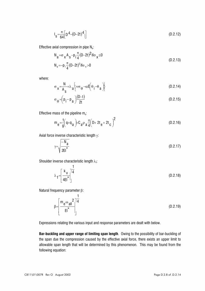
( )
−−
π= 4t2DD4
64sI (D.2.12)
Effective axial compression in pipe Na:
( )
( ) 0ift2D4
pN
0xif2t2D4ipsAxaN
x2
ia >σ−π
−=
≤σ−π
−σ= (D.2.13)
where:
θ−θα−θσνλ+=σ aiEa
sAN
x (D.2.14)
( )t2tD
apip−
−=θσ (D.2.15)
Effective mass of the pipeline me:
2
ct2et2D4aaCaqq
g1
em
++
πρ+
+= (D.2.16)
Axial force inverse characteristic length γ:
*EI2
aN−=γ (D.2.17)
Shoulder inverse characteristic length λf:
41
*EI4
vk
f
=λ (D.2.18)
Natural frequency parameter β:
41
*EI
2allem
ω=β (D.2.19)
Expressions relating the various input and response parameters are dealt with below. Bar-buckling and upper range of limiting span length. Owing to the possibility of bar-buckling of the span due the compression caused by the effective axial force, there exists an upper limit to allowable span length that will be determined by this phenomenon. This may be found from the following equation:
C811\01\007R Rev O August 2002 Page D.2.8 of .D.2.14

−
λγ−
γ< 1
2
f
1cos2
L (D.2.20)
Frequency determinant. The lowest natural frequency of the span mechanical model is computed from the frequency determinant. This is a four by four array as follows:
0
22b2
1b21a32b2
1b21a1a22
2a21b2
1a32a21b2
1a1a2
2b1a222b2
1b21a2a1a22
2a21b2
1a
2
L2bcos3
2b2
L2bsin3
2b2
L2acosh3
2a2
L2asinh3
2a
2
L2bcos2b
2
L2bsin2b
2
L2acosh2a
2
L2asinh2a
=
+−−
+
−−−
+
−+−
++−
−
−
(D.2.21)
where:
γ+
β−λ= 244
f421
1a (D.2.22)
γ−
β−λ= 244
f421
1b (D.2.23)
γ+
β+γ= 244
2a (D.2.24)
γ−
β+γ= 244
2b (D.2.25)
It will be observed that the elements of the frequency determinant are functions of γ, λf, β and L. D.2.7.7 Analysis Procedure In the analysis procedure, the span length is determined for which the lowest natural frequency of the span corresponds to the limiting natural frequency. This is achieved by fixing the values of the input parameters γ, λf and β in the elements of the frequency determinant, and computing the value of L which causes the expansion of the determinant to be zero. D.2.7.8 Analytical Method Implementation The analytical method has been implemented into a spreadsheet program. An example of an analysis proforma is given in section D.3, ATTACHMENTS.
C811\01\007R Rev O August 2002 Page D.2.9 of .D.2.14

D.2.8 ACCEPTANCE CRITERION The output from the Tier 1 dynamic strength analysis method is a computed span length Lcomp. A percentage of this is compared with the observed span length to determine acceptability of the latter; the percentage suggested is 90%. Hence, the criterion for acceptability of the observed span is:
compL9.0obsL ≤ (D.2.26)
C811\01\007R Rev O August 2002 Page D.2.10 of .D.2.14
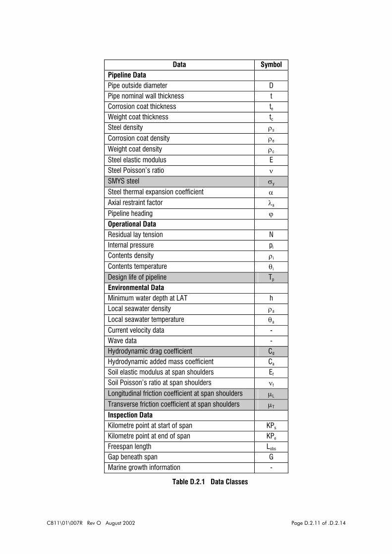
Data Symbol Pipeline Data Pipe outside diameter D Pipe nominal wall thickness t Corrosion coat thickness te Weight coat thickness tc Steel density ρs Corrosion coat density ρe Weight coat density ρc Steel elastic modulus E Steel Poisson’s ratio ν SMYS steel σy Steel thermal expansion coefficient α Axial restraint factor λa Pipeline heading ϕ Operational Data Residual lay tension N Internal pressure pi Contents density ρi Contents temperature θi Design life of pipeline Tp Environmental Data Minimum water depth at LAT h Local seawater density ρa Local seawater temperature θa Current velocity data - Wave data - Hydrodynamic drag coefficient Cd Hydrodynamic added mass coefficient Ca Soil elastic modulus at span shoulders Ef Soil Poisson’s ratio at span shoulders νf Longitudinal friction coefficient at span shoulders µL Transverse friction coefficient at span shoulders µT Inspection Data Kilometre point at start of span KPs Kilometre point at end of span KPe Freespan length Lobs Gap beneath span G Marine growth information -
Table D.2.1 Data Classes
C811\01\007R Rev O August 2002 Page D.2.11 of .D.2.14

Action Loading Load Combination
PIPELINE WEIGHT SUBMERGED SELF-WEIGHT • • • • EXTERNAL TEMPERATURE ENVIRONMENTAL: LONG-TERM • • • •
EXTERNAL PRESSURE • • • • CURRENT-INDUCED ENVIRONMENTAL: SHORT-TERM • • • •
WAVE-INDUCED • • • • CONTENTS WEIGHT •
INTERNAL TEMPERATURE NORMAL OPERATING • INTERNAL PRESSURE • CONTENTS WEIGHT •
INTERNAL TEMPERATURE MAXIMUM ALLOWABLE OPERATING • INTERNAL PRESSURE • CONTENTS WEIGHT •
INTERNAL TEMPERATURE SHUT-DOWN (MINIMUM OPERATING)
•
INTERNAL PRESSURE • CONTENTS WEIGHT •
INTERNAL TEMPERATURE HYDROTEST • INTERNAL PRESSURE •
Table D.2.2 Relationship Between Actions, Loading And Load Combinations
C811\01\007R Rev O August 2002 Page D.2.12 of .D.2.14

Parameter description Symbol Formula / note
Freespan length L Varies within analytical procedure, see subsection D.2.7.7.
Bending rigidity of pipe EI*
ν−
=21
sIE*EI
Equivalent bending rigidity, based on hoop inextensibility of pipe.
Axial force in pipe (compression entered as negative)
Na
( ) ( )2t2D4ip2t2DD2
4xaN −π
−
−−
πσ=
Effective axial force in the pipe. σx only to be included if negative; residual lay tension ignored.
Effective mass of pipeline me
++
πρ+
+= ct2et2D
4aaCaqqg1
em
Axial force inverse characteristic length
γ
*EI2
aN−=γ
Shoulder inverse characteristic length
λf 4
1
*EI4
vk
f
=λ
kf is the vertical foundation stiffnesses per unit length, see subsection D.2.7.3.
Natural frequency parameter β 41
*EI
2allem
ω=β
Based on allowable natural frequency ωall, calculated as shown in subsection D.2.6.2.
Table D.2.3 Input And Response Parameters For Tier 1 Span Mechanical Model
C811\01\007R Rev O August 2002 Page D.2.13 of .D.2.14
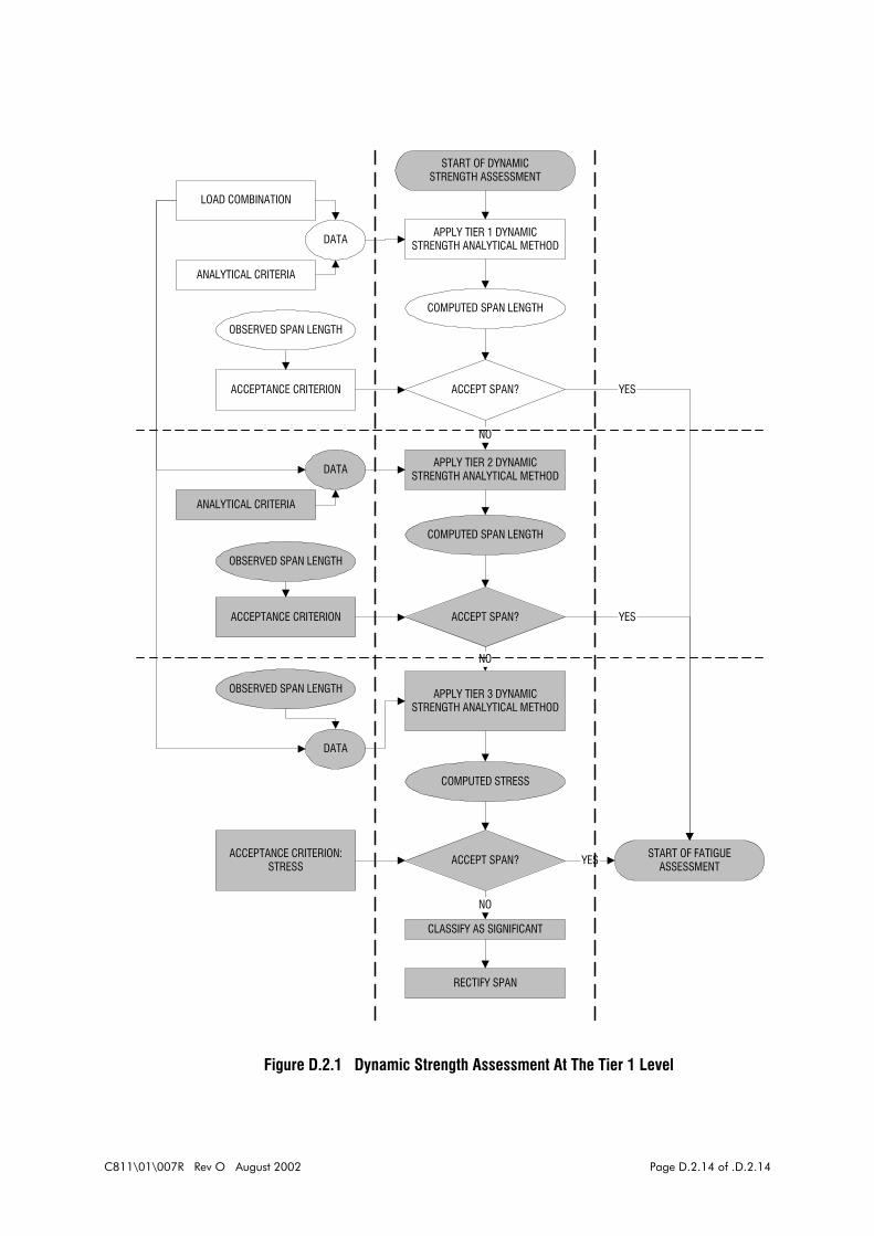
ACCEPT SPAN?
DATA
ANALYTICAL CRITERIA
LOAD COMBINATION
APPLY TIER 1 DYNAMICSTRENGTH ANALYTICAL METHOD
COMPUTED SPAN LENGTH
OBSERVED SPAN LENGTH
YES
NO
ACCEPT SPAN?
APPLY TIER 2 DYNAMICSTRENGTH ANALYTICAL METHOD
COMPUTED SPAN LENGTH
YES
NO
ACCEPTANCE CRITERION
ACCEPT SPAN?
APPLY TIER 3 DYNAMICSTRENGTH ANALYTICAL METHOD
COMPUTED STRESS
YES
NO
START OF FATIGUEASSESSMENT
CLASSIFY AS SIGNIFICANT
DATA
ACCEPTANCE CRITERION:STRESS
DATA
ANALYTICAL CRITERIA
ACCEPTANCE CRITERION
RECTIFY SPAN
START OF DYNAMICSTRENGTH ASSESSMENT
OBSERVED SPAN LENGTH
OBSERVED SPAN LENGTH
Figure D.2.1 Dynamic Strength Assessment At The Tier 1 Level
C811\01\007R Rev O August 2002 Page D.2.14 of .D.2.14

D.3 ATTACHMENTS
TIER 1 Beam on elastic foundation VORTEX SHEDDING span assessment methodPipeline data- Symbol Value (Units)Pipeline segment identification ID PL-101-AKilometre start point KPs 0 kmKilometre end point KPe 0.16 kmOutside diameter D 762 mmNominal wall thickness t 15.88 mmCorrosion coat thickness te 5.56 mWeight coat thickness
mtc 48 m
Steel density rs 7850 kg/m^3Corrosion coat density re 1200 kg/m^3Weight coat density rc 3124 kg/m^3Steel elastic modulus E 207000 N/mm^2Steel Poissons ratio nu 0.3Steel coeff. of thermal expansion alf 1.16E-05 ° C^-
Operational conditions data
m
- (Units)Residual lay tension Nlay 0 NContents pressure pnorm 1.69 N/mm^2Contents density ri 585.4 kg/m^3Contents temperature thi 15 ° C
Environmental data- (Units)Gravitational acceleration g 9.81 m/s^Minimum water depth at LAT h 37 mCurrent speed at top of pipe Vc 0.57 m/sSig. wave induced velocity at top of pipe Vwsig 0.52 m/sLocal seawater density rw 1025 kg/m^3Local seawater temperature tha 8 ° CHydrodynamic added mass coefficient Ca 1Soil elastic modulus at span shoulders kf 25 N/mm^2
Safety factors etc.- (Units)Weight growth factor ew 1Axial restraint factor l 1Threshold reduced velocity Vrth 3.5Safety factor on span (vortex shedding) llv 0.9P-delta effect switch (0 = off, 1 = on) Switch 1
Principal results- (Units)Submerged weight of pipe/unit length q 3257.9 N/mEffective mass of pipe/unit length me 1548.3 kg/mResidual lay tension stress Slt 0 N/mHoop stress Sh 30.97 N/mm^2Thermal stress St - N/mm^2Poisson effect stress Sp 9.29 N/mm^2Net prebending longitudinal stress Sn -7.52 N/mm^2Membrane axial force -2.80E+05 NBore pressure axial force -7.08E+05 NEffective axial force -9.88E+05 NAllowable frequency Fall 0.3608 HzError check on span length calculation Error OKFactored span length based on fix-fix ends 65.88 m
Factored governing allowable span length Lv1 60.3 m
Table D.3.1 Example Of Tier 1 Dynamic Strength Analysis Proforma
C811\01\007R Rev O August 2002 Page D.3.1 of D.3.1

C811\01\007R Rev O August 2002 Page E.0.1 of E.0.4
APPENDIX E
DEVELOPMENT OF FATIGUE
ASSESSMENT METHODOLOGY

C811\01\007R Rev O August 2002 Page E.0.2 of E.0.4
CONTENTS
Page No.
E.1 OVERVIEW E.1.1
E.1.1 PREAMBLE E.1.1
E.1.2 BACKGROUND CONSIDERATIONS E.1.2
E.1.2.1 Fixed Rigid Cylinders in Uniform Steady Flow E.1.2
E.1.2.1.1 Flow regime E.1.2
E.1.2.1.2 Vortex shedding E.1.3
E.1.2.2 Factors Affecting Strouhal Number for Fixed Rigid Cylinders in Uniform
Steady Flow E.1.5
E.1.2.2.1 Reynold’s number E.1.5
E.1.2.2.2 Cylinder roughness E.1.6
E.1.2.2.3 Boundary proximity E.1.7
E.1.2.2.4 Turbulence intensity in approach flow E.1.7
E.1.2.3 Elastically Restrained Rigid Cylinders in Uniform Steady Flow E.1.7
E.1.2.3.1 Modes of response E.1.8
E.1.2.3.2 Means of illustration of response E.1.8
E.1.2.4 Unsteady Flow: General Considerations E.1.10
E.1.2.4.1 Wave-induced current E.1.11
E.1.2.4.2 Combined steady and wave-induced current E.1.12
E.1.3 ANALYTICAL TECHNIQUES E.1.13
E.1.3.1 Preamble E.1.13
E.1.3.2 Reduced Velocity Techniques E.1.14
E.1.3.2.1 DNV (1981) E.1.15
E.1.3.2.2 Barltrop and Adams (1991) E.1.17
E.1.3.2.3 OTI 93 614 (HSE, 1993) E.1.18
E.1.3.2.4 APAL (1993) E.1.21
E.1.3.3 Structural Mechanics Techniques E.1.21
E.1.3.3.1 EXXON method E.1.21
E.1.3.3.2 ABAQUS E.1.22
E.1.4 LITERATURE REVIEW E.1.25
E.1.4.1 Preamble E.1.25
E.1.4.2 Fluid Loading E.1.26
E.1.4.2.1 Steady current in free stream E.1.26
E.1.4.2.2 Planar oscillatory flow E.1.27
E.1.4.2.3 Combined steady current and wave-induced flow E.1.28
E.1.4.3 Reduced Velocity Techniques E.1.31

C811\01\007R Rev O August 2002 Page E.0.3 of E.0.4
E.1.4.3.1 Steady current and planar oscillatory flow in free stream E.1.31
E.1.4.3.2 Steady current and plane boundary E.1.33
E.1.4.3.3 Planar oscillatory flow and plane boundary E.1.37
E.1.4.3.4 Steady current, planar oscillatory flow and plane boundary E.1.40
E.1.4.3.5 Steady current and scour trenches E.1.48
E.1.4.3.6 Planar oscillatory flow and scour trenches E.1.48
E.1.4.4 General Fatigue Calculations for Pipeline Spans E.1.50
E.1.4.5 Summary of Literature in Relation to Assessment Issues E.1.52
E.1.5 FATIGUE LIFE AND DAMAGE CALCULATION E.1.53
E.1.5.1 Limits Set by Codes and Guidelines E.1.53
E.1.5.1.1 BS 8010 E.1.53
E.1.5.1.2 DNV E.1.54
E.1.5.1.3 IP6 E.1.55
E.1.5.2 S-N Curves E.1.55
E.1.5.3 Damage/Fatigue Life Calculation E.1.55
E.1.6 SUMMARY AND CLOSING REMARKS E.1.56
E.1.6.1 Background Considerations E.1.56
E.1.6.2 Literature Review E.1.57
E.2 INITIAL PROPOSALS FOR DYNAMIC METHODOLOGY E.2.1
E.2.1 PREAMBLE E.2.1
E.2.2 OVERALL DYNAMIC ASSESSMENT STRATEGY E.2.1
E.2.2.1 Overall Strategy E.2.1
E.2.2.2 Deterministic, Statistical and Reliability-Based Strategies E.2.2
E.2.3 DATA, LOADING CASES AND LOAD COMBINATIONS E.2.2
E.2.3.1 Data E.2.2
E.2.3.2 Loading Classes E.2.3
E.2.3.3 Load Combinations E.2.4
E.2.4 ANALYTICAL METHODS E.2.4
E.2.4.1 Tier 1 E.2.4
E.2.4.2 Tier 2 E.2.5
E.2.4.3 Tier 3 E.2.5
E.2.5 DETAILED LOADING E.2.6
E.2.5.1 Data E.2.6
E.2.5.1.1 Current data E.2.6
E.2.5.1.2 Wave data E.2.6
E.2.5.2 Data Processing E.2.7
E.2.5.2.1 Current E.2.7
E.2.5.2.2 Wave E.2.7

C811\01\007R Rev O August 2002 Page E.0.4 of E.0.4
E.2.5.2.3 Combined current and wave data E.2.8
E.2.5.2.4 Further pre-processing E.2.9
E.3 CONCLUSIONS E.3.1
E.4 RECOMMENDATIONS E.4.1
E.5 REFERENCES E.5.1

C811\01\007R Rev O August 2002 Page E.1.1 of E.1.72
E.1 OVERVIEW
E.1.1 PREAMBLE
Figure E.1.1 presents, in generic terms, a framework outlining the key facilities necessary for
dealing with fatigue assessment of pipelines, and how these various aspects interact. In broad
terms this framework would be the same regardless of what structural system is under
consideration. The detail relating to some or all of the individual modules indicated in the figure
would render the framework particular to pipelines. Moreover, this detail would also dictate, in
an analogous way to the methodology suggested for static strength assessment, the degree
of conservatism/complexity of the modules and therefore the tier at which they should be
applied. The modules indicated in Figure E.1.1 may be described in general terms in the
following.
1. Environmental Data
This module comprises the development and manipulation of data pertaining to sea conditions.
It would involve a wide range of sea-states consisting of wave heights and periods, and
nominally steady current velocities. Data provision and manipulation would be principally
statistical.
2. Analytical Loading
The purpose of this module is to receive data generated by the preceding module and to process
it into suitable "loading" for use by the subsequent analytical module. This processing is likely
to involve two stages: firstly, the translation of conditions at the sea surface (or some other
measuring point) into water par ticle velocity conditions at the seabed, or top of pipeline level;
secondly, the conversion of water particle motions into hydrodynamic loading. Depending on
the analytical tools used, only the first or both of these stages may be necessary.
3. Analysis
This module is necessary to predict the response of the pipeline to the analytical loading derived
from the previous module given the input of structural data. A great range of analytical tools are
available, but the consideration of appropriate ones must be based on the fact that, owing to
the nature of the loading, a great deal of repeated analysis will be necessary. In any case the
analytical tool must predict the response (in terms of motion) of the pipeline span to the loading.
4. Stress Ranges
This module is required to compute the stress ranges that result in the pipeline span from its
motion. This computations may or may not be directly integrated within the previous module

C811\01\007R Rev O August 2002 Page E.1.2 of E.1.72
depending on the analytical tools employed there.
5. Fatigue Damage/Life
The procedures within this module are required to receive the stress ranges calculated from the
previous module and, using them as input data, compute the fatigue damage and life of the
pipeline span.
The preceding represents a simplified view of the problem, but nevertheless provides a valuable
framework around which the remainder of this Section of the report is built. Of the above
modules the most contentious is probably the analysis and the tools employed therein; this is
dealt with in Section E.1.3. Having laid the foundations for this in fairly detailed but more
general terms, a comprehensive review of literature is given in Section E.1.4; this is devoted
principally to identifying key information relevant to analysis methods and assessment
methodologies in general. Section E.1.5 deals with fatigue damage and life calculations and
limits imposed by codes and standards. Closing remarks, in which the information is brought
together, summarised and preliminary conclusions drawn, are given in Section E.1.6.
The hydrodynamic loading and response of pipeline spans is a highly complex phenomenon,
particularly with regard to vortex shedding. The subject area is very demanding as it involves
fluid dynamics and structural mechanics in close and complicated interaction. For this reason
it was felt important to preface all of the sections referred to above with Section E.1.2, which
covers the background considerations. These centre particularly around cylinders in fluid flow
of various types and vortex shedding, the principal factors affecting response, the key non-
dimensionalised parameters defining flow and response, and the primary means of illustrating
response. All of these provide a fundamental basis for the understanding and interpretation of
information provided in the later sections of the report.
E.1.2 BACKGROUND CONSIDERATIONS
E.1.2.1 Fixed Rigid Cylinders in Uniform Steady FlowAlthough not directly replicating in all aspects the physical reality of the problem, the body of
technological knowledge associated with the uniform steady flow of fluid around fixed rigid
cylindrical bodies forms the basis of the understanding of the dynamic response of spanning
submarine pipelines. Two particular aspects assume primary importance, namely: flow regime
(importance of Reynolds number) and vortex shedding (importance of Strouhal number).
E.1.2.1.1 Flow regime
The regimes in free-stream flow past a rigid circular cylinder depend on a non-dimensional
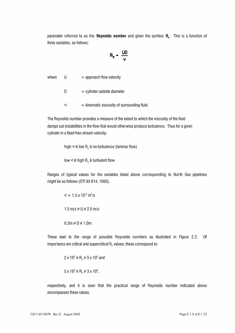
C811\01\007R Rev O August 2002 Page E.1.3 of E.1.72
parameter referred to as the Reynolds number and given the symbol, Re. This is a function of
three variables, as follows:
where U = approach flow velocity
D = cylinder outside diameter
< = kinematic viscosity of surrounding fluid.
The Reynolds number provides a measure of the extent to which the viscosity of the fluid
damps out instabilities in the flow that would otherwise produce turbulence. Thus for a given
cylinder in a fixed free-stream velocity:
high < 6 low Re 6 no turbulence (laminar flow)
low < 6 high Re 6 turbulent flow
Ranges of typical values for the variables listed above corresponding to North Sea pipelines
might be as follows (OTI 93 614, 1993).
< = 1.5 x 10⁻⁶ m2/s
1.5 m/s # U # 2.5 m/s
0.3m # D # 1.0m
These lead to the range of possible Reynolds numbers as illustrated in Figure 2.2. Of
importance are critical and supercritical Re values; these correspond to:
2 x 10⁵ # Re # 5 x 10⁵ and
5 x 10⁵ # Re # 3 x 10⁶,
respectively, and it is seen that the practical range of Reynolds number indicated above
encompasses these values.
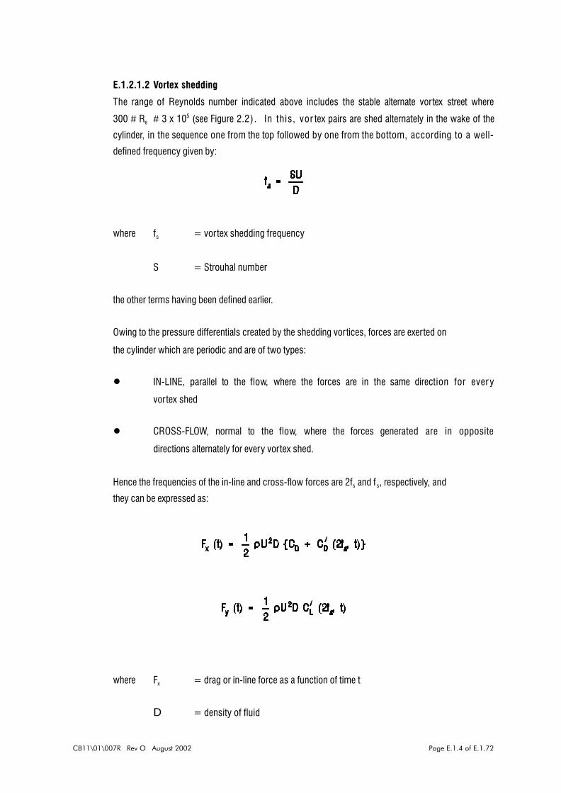
C811\01\007R Rev O August 2002 Page E.1.4 of E.1.72
E.1.2.1.2 Vortex shedding
The range of Reynolds number indicated above includes the stable alternate vortex street where
300 # Re # 3 x 10⁵ (see Figure 2.2). In this, vor tex pairs are shed alternately in the wake of the
cylinder, in the sequence one from the top followed by one from the bottom, according to a well-
defined frequency given by:
where fs = vortex shedding frequency
S = Strouhal number
the other terms having been defined earlier.
Owing to the pressure differentials created by the shedding vortices, forces are exerted on
the cylinder which are periodic and are of two types:
! IN-LINE, parallel to the flow, where the forces are in the same direction for ever y
vortex shed
! CROSS-FLOW, normal to the flow, where the forces generated are in opposite
directions alternately for every vortex shed.
Hence the frequencies of the in-line and cross-flow forces are 2fs and fs, respectively, and
they can be expressed as:
where Fx = drag or in-line force as a function of time t
D = density of fluid

C811\01\007R Rev O August 2002 Page E.1.5 of E.1.72
CD = 'steady' drag coefficient
CD' = fluctuating (time dependent) drag coefficient
Fy = lif t or cross-flow force
CL' = fluctuating (time dependent) lif t coefficient.
Clearly the shedding frequency is of prime importance and, with reference to the formula
given above for f s, central to its value is the non-dimensional parameter referred to as the
Strouhal number given the symbol S. Given the importance of this parameter the factors
affecting it are discussed in more detail in the next section.
E.1.2.2 Factors Affecting Strouhal Number of Fixed Rigid Cylinders in UniformSteady Flow
The key factors affecting Strouhal number, and consequently vor tex shedding frequency, have
been listed in OTI 93 614 (HSE, 1993), for example, as:
! Reynolds number
! Cylinder roughness
! Boundary proximity
! Velocity gradient across cylinder
! Turbulence intensity in approach flow
! Cylinder length:diameter ratio
In the case of velocity gradient, there is a trend for S to increase with increasing gradient, but
this is eliminated if the approach velocity of the fluid is taken as the value at the top of the
cylinder. The cylinder length:diameter ratio is generally considered not to be a significant
parameter in spanning situations owing to the fact that the cylinder is compliant. The remaining
factors warrant more detailed discussion, as given below.
E.1.2.2.1 Reynolds number
Information on the effects of this factor on Strouhal number for fixed rigid cylinders can be found
in Barltrop and Adams (1991), OTI 93 614 (HSE, 1993) and Sheppard and Omar (1992). A figure

C811\01\007R Rev O August 2002 Page E.1.6 of E.1.72
representing the dependence of S on Re is given in Figure E.1.3. This is fairly typical of
information given by all references in this respect; all tend to agree that there are regimes of
Strouhal number corresponding to ranges of Reynolds number. There is, however, a lack of
agreement as to the nomenclature used for the regimes and the values of Re representing the
demarcations between the regimes. This is not surprising given that these matters are a
question of interpretation of experimental data.
Also indicated on Figure E.1.3 are power spectral densities for cross-flow spectra versus
Strouhal number for a number of fixed values of Reynolds number. These are useful
because they indicate the strength of the vortex shedding (magnitudes of the ordinates) and
the concentration of values of Strouhal number (shape of curve as related to abscissae).
In terms of regimes of response the following are suggested in OTI 93 614 (HSE, 1993):
! SUBCRITICAL: 3 x 10² < Re < 2 x 10⁵, vortex shedding highly regular,
S approximately constant and equal to 0.2.
! CRITICAL: 2 x 10² < Re < 3 x 10⁵, weak vortex shedding, S approximately
equal to 0.46.
! SUPERCRITICAL: 5 x 10² < Re < 3.5 x 10 5, regular weak vortex shedding over a
broad band of frequencies, 0.4 < S < 0.46.
! TRANSCRITICAL: 3.5 x 10⁶ < Re, regular vortex shedding, S $ 0.2.
Sheppard and Omar (1992) argue that for all practical purposes vortices are shed at a single
frequency for Re < 7 x 10⁵ and for Re > 7 x 10⁶. For 7 x 10⁵ < Re < 7 x 10⁶ the spectrum of
cross-flow forces is broad-banded, reduced in magnitude and very sensitive to such things
as free stream turbulence.
E.1.2.2.2 Cylinder roughness
The preceding has considered cylinders that are hydraulically smooth. Cylinder roughness
leads to turbulence and this exerts a major influence on the process of laminar to turbulent
flow transition and hence the physical characteristics of the flow regime around the
perimeter of the cylinder. The parameter usually used to quantify roughness is the relative
roughness as given by ks/D, where k s is termed the equivalent sand roughness (and is
related to real sand grain diameters)
According to OTI 93 614 (HSE, 1993) the major effect of increasing roughness is to lower the
Re values demarcating the subcritical, critical, supercritical and transcritical regions of
C811\01\007R Rev O August 2002 Page E.1.7 of E.1.72
response described above. Within the regions themselves the following effects are
observed:
! SUBCRITICAL: vortex shedding regular, S approximately constant and equal to
0.2.
! CRITICAL: vortex shedding eliminated, region disappears for
ks/D ï> 1 x 10⁻², vortex shedding always present.
! SUPERCRITICAL: introduction of roughness re-establishes regular strong vortex
shedding, for 0.75 x 10⁻³ < ks/D < 30 x 10-3, S in the range 0.2 <
S < 0.46 and is inversely proportional to the relative roughness.
! TRANSCRITICAL: vortex shedding behaviour largely independent o f Re , S in the
range 0.21 < S < 0.23.
Summary diagrams, giving the variation of S with Re for different ks/D values and the boundaries
between the various flow regimes, are given in Figure 2.4 and are taken from OTI 93 614 (HSE,
1993). It is also wor th noting that according to this reference a typical ks value for a concrete
coated pipeline would be around 6.0mm giving a range of relative roughness between 2 x 10⁻²
and 6 x 10⁻³ for pipelines with diameters between 0.3 and 1.0m.
E.1.2.2.3 Boundary proximity
It is to be expected that the presence of a rigid plane boundar y parallel to the flow will affect the
Strouhal number. Moreover as the gap between the cylinder and the boundary is reduced the
frequency of vortex shedding (which is proportional to the effective approach velocity) and the
Strouhal number will increase. The gap ratio (ratio of gap size to cylinder diameter) is taken as
the key parameter and it has been found that the Strouhal number (for subcritical values of Re)
maximises for gap ratios of 0.5 and 0.75, with increases in the Strouhal number of the order of
5% and 10% of the free stream value.
E.1.2.2.4 Turbulence intensity in approach flow
The effects caused by turbulence in the approach flow may be classified as indirect and direct.
In the case of indirect effects, turbulence may cause changes in the flow velocity distribution
resulting in velocity gradients across the width of the cylinder; the effects of these have been
discussed above. Direct effects relate to the physical characteristics of the flow, and little is
known about this.
C811\01\007R Rev O August 2002 Page E.1.8 of E.1.72
E.1.2.3 Elastically Restrained Rigid Cylinders in Uniform Steady FlowThe preceding has considered rigid cylinders held fixed in uniform flow, a fur ther stage of
development towards similitude with a pipeline span is to allow the cylinder flexibility of motion
in the in-line and cross-flow directions. This provides the cylinder with the ability to move in
response to the hydrodynamic forces imposed upon it by the vortex shedding. Resonance of
the cylinder can interact with the vor tex shedding process, forcing the vor tex shedding into
synchronisation with the cylinder motion (at its natural frequency) thereby magnifying the
amplitude of vibration. This phenomenon is referred to as lock-in. The key point is that the
effect of cylinder motion is to enhance and actively assist in the vortex formation and shedding
process. It should be noted that the cylinder, owing to its rigidity, possesses only two degrees
of kinematic freedom corresponding with the in-line and cross-flow directions.
E.1.2.3.1 Modes of response
Given the behaviour of fixed cylinders, at least two modes of response would be anticipated for
cylinders having the ability to move, namely:
! IN-LINE, in which the frequency of vortices shed in the wake of the cylinder is
approximately equal to half the natural frequency of vibration of the cylinder
! CROSS-FLOW, in which the frequency of vor tices shed is approximately equal to the
natural frequency of vibration of the cylinder.
In the event these occur, but in addition a third IN-LINE response is possible which is associated
with the shedding of symmetric pairs of vortices, one from the top and one from the bottom of
the cylinder, simultaneously. This is a forced phenomenon, which may occur at lower flow
velocities, and is caused by low relative velocity between the moving cylinder and the flow.
E.1.2.3.2 Means of illustration of response
Generally, and particu larly with regard to the reporting of experimental work involving moveable
cylinders in uniform flow, response is illustrated graphically using dimensionless parameters.
In the case of moveable cylinders, care must be taken in distinguishing the frequency of vortices
shed in the wake of the cylinder from that of vor tices that would have been shed had the
cylinder been fixed. This is because the phenomenon of lock-in results in the fact that these
two frequencies are different under particular flow conditions.
The following frequency parameters are used:
fn = natural frequency of vibration of the moveable cylinder
fs = vortex shedding frequency for the fixed cylinder
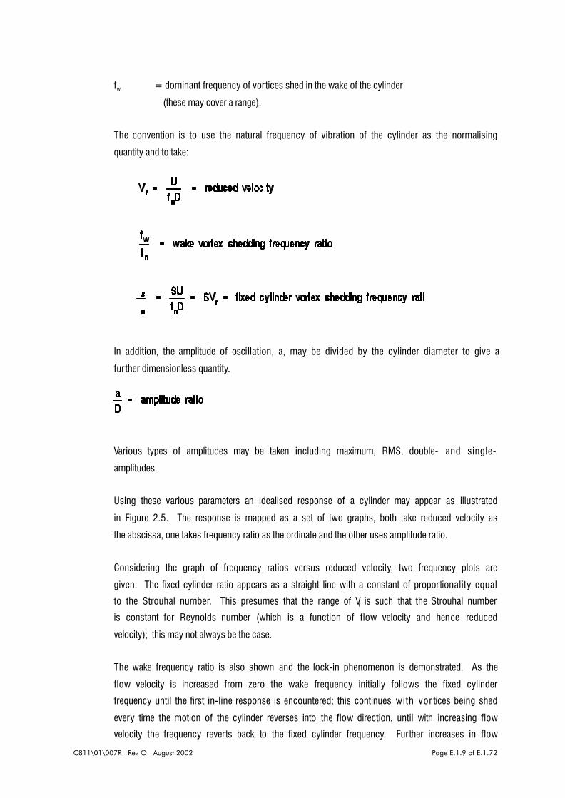
C811\01\007R Rev O August 2002 Page E.1.9 of E.1.72
fw = dominant frequency of vortices shed in the wake of the cylinder
(these may cover a range).
The convention is to use the natural frequency of vibration of the cylinder as the normalising
quantity and to take:
In addition, the amplitude of oscillation, a, may be divided by the cylinder diameter to give a
further dimensionless quantity.
Various types of amplitudes may be taken including maximum, RMS, double- and single-
amplitudes.
Using these various parameters an idealised response of a cylinder may appear as illustrated
in Figure 2.5. The response is mapped as a set of two graphs, both take reduced velocity as
the abscissa, one takes frequency ratio as the ordinate and the other uses amplitude ratio.
Considering the graph of frequency ratios versus reduced velocity, two frequency plots are
given. The fixed cylinder ratio appears as a straight line with a constant of proportionality equal
to the Strouhal number. This presumes that the range of Vr is such that the Strouhal number
is constant for Reynolds number (which is a function of flow velocity and hence reduced
velocity); this may not always be the case.
The wake frequency ratio is also shown and the lock-in phenomenon is demonstrated. As the
flow velocity is increased from zero the wake frequency initially follows the fixed cylinder
frequency until the first in-line response is encountered; this continues with vor tices being shed
every time the motion of the cylinder reverses into the flow direction, until with increasing flow
velocity the frequency reverts back to the fixed cylinder frequency. Further increases in flow

C811\01\007R Rev O August 2002 Page E.1.10 of E.1.72
veloci ty result in lock-in to the second in-line case where it is seen that the wake frequency
remains equal to half the natural frequency of the cylinder over a range of flow velocities. Within
this range the actual Strouhal number is reduced by wake circulation, which is built up by the
cylinder motion, allowing the wake frequency to be maintained at half the cylinder natural
frequency. Eventually a flow velocity is reached where sufficient circulation to achieve this
cannot be preserved and a jump back to the fixed cylinder frequency occurs. This situation is
maintained until the cross-flow lock-in occurs, for which the mechanisms are similar to those
just described, except that over the range of flow velocity corresponding to lock-in the wake
frequency is maintained at the cylinder natural frequency.
It is seen that, in general, at lock-in enforced synchronisation over-rides fixed cylinder theory.
This is also illustrated by the plot of amplitude ratio versus reduced velocity where it is seen that
lock-in is characterised by a series of peaks in the curve that maximise then die away at ranges
of flow velocity for which the wake frequency coincides with the fixed cylinder vortex shedding
frequency. Given that peaks occur, this indicates that the amplitudes of vibration of the cylinder
may be limited in both the in-line and cross-flow directions as a result, say, of mechanical
damping in the system. However, during the lock-in phases, the forces applied to the cylinder
may be greater than those exerted on fixed cylinders.
The description above represents a somewhat idealised situation in which the modes of
response are well-separated and distinguishable. In practice significant response may occur
well before cross-flow resonance takes place and in addition to this coupled vibration between
in-line and cross-flow motions may occur, giving, depending on oscillation frequencies, elliptical
or figure of eight vibration orbits (Lissajous figures).
E.1.2.4 Unsteady Flow: General ConsiderationsIn all the preceding, consideration has been confined to uniform steady flow, ie. the free stream
flow velocity does not change with time. In practice currents incident upon a suspended length
of pipeline will not, in general terms, be as simple as this. They will comprise flow velocities
derived from the following:
! tidal flows, usually based on a long period of variation and, therefore, treated as
quasi-static
! storm surge and other similar transient events
! wave-induced, involving a whole spectrum of periods.
In fatigue terms the most important of these will be the more frequently occurring events, ie. the
steady current arising from tidal flows, and the flow velocities stemming from waves. Since

C811\01\007R Rev O August 2002 Page E.1.11 of E.1.72
steady flow has been dealt with already it remains to address the background considerations
pertaining to wave-induced currents, and the combination of steady and wave-induced currents.
E.1.2.4.1 Wave-induced current
In the course of wave action water par ticle orbits are elliptical in one wave period. Precise orbit
shapes depend upon wave period and mean water depth. In deep water, particle orbits are
circular having diameters which decrease exponentially towards the seabed to the extent that
the water at depths in excess of about one half of a wavelength is hardly affected by waves.
In shallow water the orbits become elliptical with their long axis parallel to the mean water
surface; at the seabed the excursions made by the water particles in the vertical direction are
virtually zero.
This latter situation means that water par ticles move only horizontally backwards and forwards
according to the periodic characteristics of the wave. This type of flow is referred to as plane
oscillatory motion, having no velocity component in the vertical direction, and is frequently used
in experimental investigations to simulate wave effects.
Of paramount impor tance is the maximum distance moved by a water particle from the centre
of the cylinder during a complete wave cycle. This is also known as the excursion. Thus during
a complete wave cycle a water particle will star t from an excursion point with zero velocity travel
past the centre of the cylinder, reach the opposite excursion point (thereby completing a wave
half-cycle), before reversing direction and returning to its starting point and completing the wave
cycle. Hence during a wave half-cycle the water particle concerned travels in the same
direction, but with a sinusoidally varying velocity. The key points in this respect are whether
there is sufficient time or distance (in terms of two excursions per wave half-cycle) and flow
velocity during a wave half-cycle to allow vor tex shedding to occur and the number that will be
shed if conditions are conducive.
This can be assessed by means of a dimensionless parameter referred to as the Keulegan-
Carpenter number and given the symbol Kc.
This is a function of two variables, as follows:
where Uw = peak flow velocity past the cylinder during a wave cycle
T = wave period

C811\01\007R Rev O August 2002 Page E.1.12 of E.1.72
D = cylinder diameter.
It is, in effect, similar in form to the reduced velocity for steady flow with the difference being
it embodies wave frequency. Indications from experimentation (OTI 93 614: HSE, 1993) are as
follows:
! Kc < 5 vor tices are shed if at all in a symmetric pattern, cross-flow
forces are insignificant
! 5 < Kc < 15 single vor tex shed in each wave half-cycle, cross-flow frequency
equals twice wave frequency
! 15 < Kc < 25 two vortices shed per wave half-cycle, dominant frequency of
cross-flow force equals three times wave frequency
! Kc > 25 increases in the number of vor tices completely formed and shed
in each wave half-cycle until wake resembles steady flow
situation, and thus becomes independent of wave frequency.
For situations where Kc is greater than 25 spectral analysis of cross-flow forces shows that
there are peak contributions at integer multiples of the wave frequency. However, the vortex
shedding is closely synchronised and coupled with the wave frequency only for Kc < 25.
There is fur ther evidence to suggest that for "high" (>20) values of Kc a form of "quasi-static"
vor tex shedding occurs where the shedding frequency closely follows the instantaneous cyclical
variations in the oscillating flow velocity. Also the wave Strouhal number (for surface roughened
cylinders) shows little Reynolds number dependence, remaining essentially constant at about
0.2. In essence this means that the formula given in Section 2.2.1 for the computation of the
vortex shedding frequency could be used by substituting the instantaneous velocity for the
steady flow velocity.
E.1.2.4.2 Combined steady and wave-induced current
In this situation it is clear that the flow velocity may or may not reverse direction depending on
the relative values of the steady and peak oscil lator y components of the flow velocity. The
overall velocity conditions may be quite different in the two halves of a wave cycle and it is
convenient to compute the Keulegan-Carpenter numbers corresponding to each wave half-cycle
in the following manner:

C811\01\007R Rev O August 2002 Page E.1.13 of E.1.72
where Uc = the steady current velocity,
and the other terms have been defined previously.
Clearly if Uc > Uw no flow reversal takes place and whilst the vor tex generation process may
vary during the course of a wave cycle, the wake remains on one side of the cylinder. Quasi-
steady flow conditions may prevail providing that the two Keulegan-Carpenter numbers
pertaining to the wave half-cycles are sufficiently high.
There is likely to be, however, a reasonable consistency in vor tex generation during the entire
wave cycle.
On the other hand if Uc < Uw the potential exists for the flow velocity to reverse direction during
part of the wave cycle. This will inevitably disrupt any vortex generation built up over a
preceding period because the upstream and wake regions relative to the cylinder, and the
velocity regimes are forced to change. Again the Keulegan-Carpenter numbers in each wave
half-cycle could be computed but values of Uc and Uw may be such as to yield a negative Kc in
one case: this should be interpreted as pertaining to a reversed velocity relative to the other
wave half-cycle. If the Keulegan-Carpenter numbers pertaining to one or both wave half-cycles
are sufficiently high, quasi-steady conditions may prevail.
E.1.3 ANALYTICAL TECHNIQUES
E.1.3.1 PreambleIt evident from a preliminary appraisal of the literature that two types of analytical techniques
either are, or have the potential to be, used in assessment of fatigue in pipeline spans. These
may be classified as techniques related to:
! reduced velocity (see Section E.1.3.2)
! structural mechanics.
Reduced velocity techniques are empirical and exploit the fact (observed in Section E.1.3.2) that
it is very of ten the case in experiments that cylinders subject to fluid flow experience limited
C811\01\007R Rev O August 2002 Page E.1.14 of E.1.72
amplitudes of vibration. The techniques utilise databases (in the broadest sense) of
experimental results to assess in the case of pipelines, firstly, the expectation of significant
dynamic response and, secondly (if this is the case) the likely maximum amplitudes of
vibration. Two important points must be made regarding this:
! experimentation tends to be predominated by tests on rigid fixed or elastically-
mounted cylinders subjected to fairly simplified flow regimes, with comparatively little
information related to real pipeline spans
! the techniques give no direct information about stress ranges.
Structural mechanics techniques embody all the dynamic str uctural analysis that may be
available. Broadly speaking these may be classified into two types, namely: time-domain and
frequency-domain analyses. They are fundamentally different and this affects their
practicability in application to fatigue calculations.
In essence time-domain analyses take a time-var ying loading applied to a structural model and
compute the response history of the model. The response history may be thought of as a graph
of stress, deflection etc., versus time. The method is very powerful, can involve structural and
material nonlinearities and so forth, and is useful in investigating the instantaneous response
of the structural model. It is not, however, a very practical method in fatigue calculations as it
does not allow the computation of stress ranges and their frequencies of occurrence directly.
Frequency-domain analyses, on the other hand, are much more suitable for fatigue
computations. The time-varying loading is broken down into its frequency components, each
component applied separately and a steady-state response calculated at that frequency. The
responses can then be superposed to give the resultant effect, or used individually in fatigue
damage calculations because stress ranges can be an automatic product of the analysis. By
its nature frequency- domain analysis is a linear dynamic technique, but this does not represent
a serious drawback in practical terms.
Structural mechanics techniques may also embody all the bespoke methods developed and
programmed on an individual basis by various companies; for example, Snamprogetti (1994).
E.1.3.2 Reduced Velocity TechniquesTechniques of this type are principally empirical and use incident flow velocity of the moving
stream of water, natural frequencies of vibration of the pipeline span, pipeline outside diameter,
pipeline effective mass per unit length, logarithmic decrement of structural damping and
seawater density in a pair of dimensionless parameters, namely: reduced velocity and a stability
parameter. These coefficients are then related to databases of experimental results, usually

C811\01\007R Rev O August 2002 Page E.1.15 of E.1.72
in graphical form, to assess:
! the expectation of significant in-line and cross-flow dynamic response
! the likely maximum amplitudes of vibration pertaining to in-line and cross-flow
vibration.
Approaches of this sort should be regarded as semi-qualitative, although attempts have been
made to use them in a more quantitative context to calculate fatigue life.
E.1.3.2.1 DNV (1981)
The guidance given in DNV (1981) is the oldest extant and is contained in Appendix A of the
document; it relates to vortex shedding due to current only. Two sets of two graphs are
provided per taining to in-line and cross-flow motions. In each set the first graph is used to
estimate the flow velocity at which motion is initiated for a particular natural frequency of
vibration of the pipeline, and the second graph is used to estimate the amplitude of vibration as
a proportion of the pipeline diameter.
The procedure is illustrated schematically in Figure 2.6. The key parameters with regard to the
procedure are as follows:
where Vr = reduced velocity (dimensionless)
Uc = incident current velocity normal to the axis of the pipeline
D = pipeline outside diameter
fi = pipeline natural frequency
where ks = stability parameter (dimensionless)
me = effective mass per unit length of pipeline, including structural,

C811\01\007R Rev O August 2002 Page E.1.16 of E.1.72
41
L
O
4
L
O
2
maxdx (x)y
dx (x)y y
=γ
∫∫
contents and added mass
* = logarithmic decrement of structural damping
D = mass of surrounding seawater
where Re = Reynolds number (dimensionless)
< = kinematic viscosity of surrounding seawater
where y = mode shape corresponding with the natural frequency concerned
ymax = maximum value of the mode shape
x = distance along a span of length L.
As can be seen from the flow chart, the processes pertaining to in-line and cross-flow
motions can be treated separately and their respective logics are derived from the underlying
graphs given in Figure E.1.7. After computation of the ks and Vr parameters, in-line motion is
considered first and reference is made to A.4 in Figure E.1.7; no significant motion occurs if
ks $ 1.8.
If, however, 1.2 # ks < 1.8 it is apparent from A.3 that motion occurs if Vr $ 2.2, whereupon the
maximum amplitude as a proportion of diameter can be read off A.4; no motion occurs if Vr <
2.2. Alternatively, if ks < 1.2 then A.3 must be checked to determine if the combination of Vr
and ks is such as to cause motion. If this is the case, then A.4 is used to determine amplitude;
if not then no significant motion needs to be taken into account.
When cross-flow motion is considered, then additional computation of Reynolds number is
necessary. No significant motion occurs if Vr < 3.7. If this is not the case, A.5 is used to
C811\01\007R Rev O August 2002 Page E.1.17 of E.1.72
determine if motion occurs, based on Re and Vr , with A.6 used to estimate the maximum cross-
flow amplitude if this is the case.
It is worth pointing out that for a given geometrical configuration of pipeline span (ie. fixed span
length) subject to a fixed current velocity, if no in-line or cross-flow motion occurs for the lowest
natural frequency of vibration then higher frequencies do not need to be investigated. However,
if motion is indicated for the lowest natural frequency, then the higher frequencies need to be
assessed until one is reached for which no motion results.
E.1.3.2.2 Barltrop and Adams (1991)
Vortex shedding is covered in Barltrop and Adams (1991), and although broadly directed towards
the dynamics of fixed marine structures it provides a comprehensive reference. The procedure
distilled from this reference is summarised in Figure E.1.8 and is broadly similar to and uses the
same assessment parameters as DNV (1981).
The procedure is governed by an overall loop in which all natural frequencies of vibration are
checked until one is reached for which no in-line or cross-flow response is indicated. For an
individual natural frequency the reduced velocity is checked against criteria to assess whether
vibration is likely to occur; if this is the case, then the amplitude of vibration as a proportion of
the pipeline diameter is read off a graph (see Figures E.1.9 and E.1.10). In-line and cross-flow
motion are both treated similarly.
Key differences exist between this method and the one suggested by DNV (1981), these relate
to:
! the assessment of the onset of motion
! the treatment of wave loading.
In terms of the onset of motion, Barltrop and Adams give fixed values to the ranges of reduced
velocity within which the oscillation modes occur. DNV on the other hand indicate that the
ranges are functions of the stability parameter ks and Reynolds number Re in the cases of in-line
and cross-flow vibrations, respectively.
Barltrop and Adams emphasise that considerable uncertainty exists when assessment is
required for wave or simultaneous wave and current forces. The central question surrounding
wave motion is whether, under velocity variation or reversal every half wave cycle, conditions
prevail to allow the build-up of vortex shedding to the same extent that might occur under steady
flow conditions.

C811\01\007R Rev O August 2002 Page E.1.18 of E.1.72
In terms of wave-only, Barltrop and Adams argue that the Keulegan-Carpenter number (see
Subsection E.2.2.4.1) is the key parameter determining whether the flow excursion is sufficient
for separation to occur and for vortices to fully form before flow reversal. For Keulegan-
Carpenter numbers in the range 0 < Kc < 5, vortices are shed (if at all) in a symmetric pattern
and cross-flow forces are insignificant.
To account for transient behaviour it is suggested that use is made of a factor denoted as Q
which deals with intermittent lock-in through the wave cycle. This is indicated on the flow chart
in Figure E.1.8 and is introduced as a division in the stability parameter ks. The computation of
Q is based on the assumption that the cyclic wave loading leads to intermittent lock-in over the
times when the velocity is in the range for excitat ion of a par ticular mode of vibration. The
response reaches an equilibrium in which the decay between periods of lock-in just balances
the increase during lock-in; on this basis Q is taken as:
where * = logarithmic decrement of structural damping
F = number of forcing cycles in a half wave cycle
M = number of decay cycles in a half wave cycle
where Tw = wave period
Tn = natural period of vibration of the pipeline.
Generally speaking in situations of intermittent lock-in the factor Q assumes a value less than
unity. This results in an increase in the stability parameter with a consequent reduction in the
amplitude vibrations computed from Figures E.1.9 and E.1.10.
E.1.3.2.3 OTI 93 614 (HSE, 1993)
This document takes a similar approach to that given in DNV (1981), but has a number of
fundamental differences. The methodology is based principally upon a number of rigorously
C811\01\007R Rev O August 2002 Page E.1.19 of E.1.72
performed full-scale experiments on smooth and roughened pipeline spans reported in OTI 92
555 (HSE, 1993) and performed by Hydraulic Research Limited in the Severn Estuary.
OTI 93 614 (HSE, 1993) argues that the reduced velocity approach of, for example, DNV (1981)
for the assessment of a span condition is not acceptable, since the characteristics of real span
behaviour are not adequately represented. The essence of the argument lies in the fact that the
simplistic view of response, that oscillations of the pipeline can be distinguished into distinct,
well-separated regimes of behaviour according to the magnitude of reduced velocity, is not
borne out by the full-scale experimental results.
In the case of smooth pipelines, hysteresis effects were found to occur in the wake frequency
response. In these, dynamic jumps took place between responses associated with in-line and
cross-flow vortex shedding frequencies with both increasing and decreasing reduced velocity.
Observations showed, however, that the spans responded at an approximately constant
frequency (nominally the still water natural frequency) throughout the changing regimes of
vortex shedding. It was also shown that whilst the initial response region was marked by in-line
vibrations, this was accompanied by smaller amplitude, but significant, cross-flow components.
Moreover, the tests revealed a significant increase in in-line response amplitude over commonly
suggested limiting values. This was ascribed to the fact that critical flow conditions gave rise
to much lower CD values than would normally be expected, the consequences of which being
that the in-line damping components due to hydrodynamic drag were reduced, thereby
increasing the corresponding vibration amplitude.
Initial findings from the experiments on stationary rough pipeline spans gave reason to expect
that the dynamic behaviour of a span at low gap ratios (ratio of gap between the underside of
the pipeline and the seabed, and the pipeline diameter G/D) differed from the behaviour for larger
gap ratios due to differences in the characteristics of the vortex-induced excitation mechanisms.
This expectation was borne out by the experiments in which spans were free to vibrate. In the
case of high gap ratios, progressive (rather than dynamic) wake frequency variations with
reduced velocity were observed between responses associated with in-line and cross-flow
vortex shedding frequencies. The span response was much more complex than in the case of
smooth pipelines: initially the span responds to increasing reduced velocity such that motions
in both the in-line and cross-flow directions are at the span still water natural frequency; for
fur ther increases in reduced velocity the in-line span response exhibits a dynamic jump in order
to remain synchronised with the wake frequency, whilst the cross-flow response maintains
synchronisation with twice the wake frequency. This sequence of events is essentially retraced
upon reduction of reduced velocity.
For small gap ratios in conjunction with rough pipelines some similarities to the responses of
smooth pipelines were exhibited but differences were observed. Upon increasing the reduced
C811\01\007R Rev O August 2002 Page E.1.20 of E.1.72
velocity an abrupt jump to a higher frequency is displayed by the wake response; following this
jump the span responds in both the in-line and cross-flow directions at roughly the still water
natural frequency.
In terms of practical response characteristics, the report recommended the following:
! the relationships for in-line motion in, for example, DNV (1981) should remain
applicable
! the cross-flow onset thresholds in DNV (1981) are judged to be non-conservative for
full-scale pipelines spans and, owing to the possibility of hysteresis effects and the
coupled interaction between the motions in the in-line and cross-flow directions
leading to an early threshold of large amplitude response, limitations should be based
solely on a reduced velocity criterion as related to gap ratio
! the incident velocity to be used for assessment should be based on the conservative
assumption of adding the steady current velocity to the maximum wave induced
velocity.
Based upon this, the potential for a pipeline span to undergo vortex-induced vibration should be
assessed using the reduced velocity parameter Vr against two threshold limits V r1 and V r2, as
follows:
Vr < Vr1 No significant vortex-induced vibration takes place
Vr1 # Vr < Vr2 Vortex-induced vibration of relatively low amplitude may take place
Vr2 # Vr Large amplitude and potentially catastrophic vor tex-induced vibration may
take place.
Vr1 is derived from A.3 of Figure E.1.7 and Vr2 is given by:
Vr2 = 2.4 if G/D # 2.0
Vr2 = 3.0 if G/D > 2.0
In cases where Vr1 # Vr < Vr2 the amplitude of response may be estimated from A.4 in Figure
2.7, and it is to be emphasised that there is no provision for amplitude calculation in the
situation when Vr2 # Vr.
The procedure thus follows the flowchart depicted in Figure E.2.11; this is similar to that in

C811\01\007R Rev O August 2002 Page E.1.21 of E.1.72
Figure 2.6 except that complete distinction is not made between in-line and cross-flow motions.
E.1.3.2.4 APAL (1993)
This particular reference suggests a fatigue methodology based around the use of the graphs
provided in DNV (1981) or the data on response amplitudes given in OTI 92 555 (HSE, 1993).
No provision is made for dealing with waves and current velocity only is considered.
The fatigue calculation consists of a basic loop which is repeated for all of a finite number of
current velocities as defined in a probability distribution function, ie. from current velocity scatter
data. Thus each current velocity taken has a probability of occurrence associated with it.
The basic loop involves carr ying out the DNV (1981) assessment procedure as described earlier
in terms of critical reduced velocities, and using either the DNV (1981) graphs, or the data set
in OTI 92 555 (HSE, 1993) to estimate the corresponding amplitudes of vibration in the in-line
and cross-flow directions. These are then combined to estimate the peak stress range and from
this an endurance limit from a suitable S-N curve. The computation is performed using the
lowest natural frequency of vibration of the pipeline span, firstly to compute the reduced velocity
at the head of the process, and finally to estimate the number of cycles actually undergone as
the product of the natural frequency and the probability of occurrence of the current velocity
under consideration. The ratio of the actual number of cycles to the endurance limit gives the
contribution made to the total fatigue damage by the particular current velocity considered.
The total fatigue damage will be the sum of all the individual contribution made by the current
velocities as defined in the probability distribution function. The damage will be in effect a rate
per length of time used in the derivation of the current velocity probability distribution function.
It is worthwhile noting that no indication is given in this document as to whether, within an
individual current velocity calculation, attention should be given to higher frequencies of vibration
of the pipeline span as indicated in the preceding subsections. Finally, the above methodology,
or an extension thereof, appears to form the basis of the assessment procedures outlined by
Kaye, Galbraith, Ingram and Davies (1993).
E.1.3.3 Structural Mechanics Techniques
E.1.3.3.1 EXXON method
This particular paper, by Pantazopoulos et al (1993) (all staff members at Exxon Production
Research Company, Houston), is significant principally for its usage of a vor tex induced loading
formulation that involves combined steady and wave-induced current. This particular aspect is
dealt with in detail in Section E.2.4.3 of this report.

C811\01\007R Rev O August 2002 Page E.1.22 of E.1.72
In addition to this, however, the paper advocates the use of a frequency-domain technique for
the solution of beam-column equations of motion used to model the response of the pipeline
span. These are two in number, corresponding to the in-line and cross-flow directions, and the
respective responses are coupled by vir tue of relative velocity effects between the moving
pipeline and the flow.
In essence the loading, as a function of time, is decomposed into its Fourier components, ie.
loading amplitudes at a series of frequencies of oscillation. The solutions, in terms of deflected
shapes, for each loading frequency are taken to be the superpositions of the eigenfunctions of
the beam-column multiplied by unknown deflection response amplitudes. The deflection
amplitudes are then determined using the equations of motion. This yields the response of the
pipeline to a loading amplitude of a fixed frequency in terms of steady state amplitude of
deflection, which can readily be converted to stress ranges for subsequent analysis for fatigue
damage or life. This process can be repeated for as many frequency components of the loading
as are deemed necessary for an accurate representation of behaviour.
It should be noted that this analytical technique is, in fact, a fairly standard type of approach
that may be determined from many textbooks on str uctural dynamics or mechanical vibrations.
What makes this particular paper stand out, however, is the use of this method in combination
with a novel loading representation as described later.
E.1.3.3.2 ABAQUS
ABAQUS is a very powerful, general purpose finite element analysis package. It is capable of
linear and nonlinear calculations involving geometric (large deflections) and material (plasticity)
effects. BOMEL has used it successfully in pipeline applications, both in terms of static
strength (BOMEL 1996a and 1996c) and in the computation of natural frequencies of vibration
(1996d).
It should be emphasised that ABAQUS is an analytical tool, and so has no facility for applying
criteria in a direct manner to limit the configuration of the system being analysed. In the case
of static strength assessments of pipeline spans the procedure adopted by BOMEL was to
increase the span length of the pipeline being considered, repeatedly analyse, and monitor key
variables (stress, strain etc) against criteria. A similar procedure has been adopted by BOMEL
for the computation of natural frequencies. This approach is successful in both these situations
providing that the number of analyses to be performed is not too large.
ABAQUS has no facility for the computation of fatigue damage, but its strength lies in its wide
range of capabilities in dynamic analysis. Broadly speaking dynamic analyses may be divided
into two types: linear and nonlinear, in much the same way as static analyses. Facilities exist
in ABAQUS for conducting frequency-domain or time-domain analyses.
C811\01\007R Rev O August 2002 Page E.1.23 of E.1.72
Linear analyses are described as linear per turbation procedures; generally this means that they
are small deflection, elastic material responses about some base state. The base state may
have been arrived at by means of a nonlinear procedure, however. In the case of the analyses
undertaken by BOMEL, natural frequencies of vibration were computed via a linear procedure
af ter having applied a nonlinear static analysis to simulate the response to the applied load. In
this way the effects of membrane tension on natural frequency were evaluated.
Within linear dynamic analyses four options are provided, namely: response spectrum analysis,
time history analysis, steady-state response analysis and random response analysis.
Response spectrum analysis provides an estimate of the peak response of a structure to
steady-state dynamic motion of its fixed points: ie. base motion. All points constrained by
boundary conditions are assumed to move in phase in any one of three orthogonal directions
(two, in planar models) according to user-specified input spectra. These spectra are defined
as functions of frequency for different values of damping. The peak responses are first
computed independently for each direction of excitation for each natural mode of vibration of the
system, which are then combined to create an estimate of the actual peak response of any
variable chosen for output, as a function of frequency and damping.
Time history analysis gives the response of a model as a function of time, based on a specified
time-dependent loading. The response is obtained from a procedure in which the model
amplitudes are integrated through time and synthesised. So long as the system under analysis
is correctly represented by the vibration modes being used (which are generally only a small
subset of the total modes of the finite element model), and the forcing functions vary piecewise-
linearly through time (achievable by means of a small enough timestep), the method can be
very accurate.
Steady-state response analysis provides the response of the system when it is excited by
harmonic loading at a given frequency. Usually such analysis is done as a frequency sweep,
by applying the loading at a series of different frequencies and recording the response. The input
for the procedure allows for such sweeping, also enabling sampling points on the frequency
scale to be spaced closer together at the natural frequencies of the system, thus allowing
detailed definition of the response close to resonance.
Random response analysis predicts the response of a system which is subjected to a
nondeterministic continuous excitation that is expressed in a statistical manner using a power
spectral density function. In the most general case this type of excitation is defined as a
frequency dependent power spectral density matrix, giving the correlation between the loadings
at the various degrees of freedom to which the excitation is applied. It is assumed by ABAQUS
that the frequency dependence and the spatial dependence of the loading can be separated.

C811\01\007R Rev O August 2002 Page E.1.24 of E.1.72
The random response of the model is expressed as power spectral density values of nodal and
element variables, as well as their root mean square values.
When nonlinear dynamic response is being studied, in which large geometrical deflections and
material plasticity must be accounted for in the analysis, direct integration of the system must
be used. All of the equations of motion of the system must be integrated through time, and
because of this, direct integration methods are generally significantly more expensive than the
modal methods that are usually chosen for linear studies (see above). Within the general
category of nonlinear dynamic analysis ABAQUS provides three methods, referred to as: direct
method, subspace projection method and explicit method.
The "standard" direct method is an implicit one, meaning that the nonlinear dynamic equilibrium
equations must be solved at each increment of time. This is done iteratively, using either
Newton's method or the quasi-Newton method. This equation solving process is expensive, but
because nonlinearities are usually more simply accounted for in dynamic situations (because
the inertia terms provide mathematical stability to the system) the method is successful in all
but a few cases of extreme nonlinearity. The principal advantage of this method lies in the fact
that variable-length time increments may be used during the course of an analysis, enabling in
some cases of sudden events, a long time record to be analysed.
In the case of the subspace projection method the eigenmodes of the linearised system are
used as a small set of global basis vectors. For some cases this method can be very effective,
and is of ten significantly less expensive than the direct integration of all the equations of motion
of the model. Within ABAQUS the method is implemented using a central difference operator
to integrate the equations of motion projected onto the eigenmodes of the linear system. A fixed
time increment is used throughout an analysis which is the smaller of a user-specified value
or one derived from the highest frequency of the eigenmodes that are used as the basis of the
solution. The effectiveness of the method depends on the value of the eigenvectors of the linear
system as a set of global interpolation functions for the problem. This relies on judgement on
the part of the user analogous to deciding the sufficiency of a particular mesh of finite elements.
The method is, however, valuable for mildly nonlinear systems.
The explicit method uses a central difference scheme but is subject to a maximum time
increment that can be taken without the method generating large, rapidly growing errors. This
is closely related to the time required for a stress wave to cross the smallest element dimension
in the model; thus the time increment may be very short if the finite element mesh contains
small elements, or if the stress wave propagation velocity in the material is high (for steel this
is 5000 m/s). The method is only computationally attractive for problems where the total
dynamic response time that must be modelled is only a few orders of magnitude longer than
this maximum time-step limit. There are also limitations in the implementation of the method

C811\01\007R Rev O August 2002 Page E.1.25 of E.1.72
with respect to the types of elements that may be used.
Broadly speaking the use of a tool like ABAQUS requires a definition of the loading. This could
be done by means of, for example, the Exxon loading model (see 2.4.3, below) or exploiting the
potential to couple the program to computational fluid dynamics (CFD) software.
E.1.4 LITERATURE REVIEW
E.1.4.1 PreambleAs stated earlier, the purpose of this subsection of the report is to perform a comprehensive
review of literature relevant to the dynamic response of pipeline spans, with a view to identifying
key information relevant to analysis methods, and assessment methodologies in general. The
approach taken has been to appraise information that usefully contributes both in terms of direct
application, (ie. specific formulations that may be used), and in a phenomenological sense, ie.
that provide behavioural understanding as a precursor to model development.
In assessing the information it is useful to have an overall appreciation of the important issues
that bear on the problem, and the way that they interact. This appreciation may be gained from
Figure E.1.12, which represents some of the major issues that require consideration in the
dynamic response of pipeline spans. Owing to the enormous complexity that the problem
presents, the great majority of the work that has been carried out by researchers has been
experimental, with a comparatively small amount that could be described as theoretical. For this
reason it is the experimental work that has dictated the choice of upper-level issue categories
indicated on the figure, namely:
! flow conditions
! cylinder type
! degrees of kinematic freedom
! seabed effects.
Other, more arcane effects stemming from detailed fluid dynamics considerations, for example:
Reynolds number, sur face roughness, turbulence and so forth, have been dealt with in
Subsections E.1.2 and E.1.3.
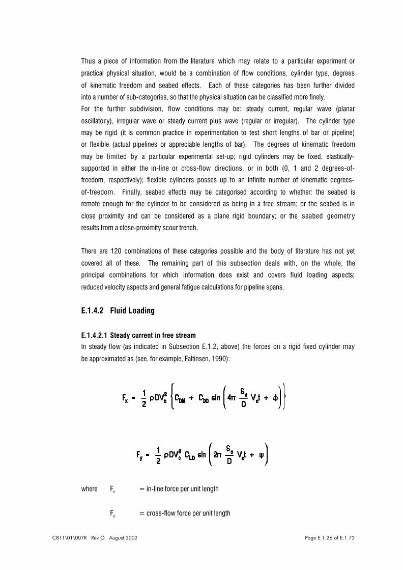
C811\01\007R Rev O August 2002 Page E.1.26 of E.1.72
Thus a piece of information from the literature which may relate to a par ticular experiment or
practical physical situation, would be a combination of flow conditions, cylinder type, degrees
of kinematic freedom and seabed effects. Each of these categories has been further divided
into a number of sub-categories, so that the physical situation can be classified more finely.
For the fur ther subdivision, flow conditions may be: steady current, regular wave (planar
oscillatory), irregular wave or steady current plus wave (regular or irregular). The cylinder type
may be rigid (it is common practice in experimentation to test short lengths of bar or pipeline)
or flexible (actual pipelines or appreciable lengths of bar). The degrees of kinematic freedom
may be limited by a par ticular experimental set-up; rigid cylinders may be fixed, elastically-
supported in either the in-line or cross-flow directions, or in both (0, 1 and 2 degrees-of-
freedom, respectively); flexible cylinders posses up to an infinite number of kinematic degrees-
of-freedom. Finally, seabed effects may be categorised according to whether: the seabed is
remote enough for the cylinder to be considered as being in a free stream; or the seabed is in
close proximity and can be considered as a plane rigid boundary; or the seabed geometry
results from a close-proximity scour trench.
There are 120 combinations of these categories possible and the body of literature has not yet
covered all of these. The remaining part of this subsection deals with, on the whole, the
principal combinations for which information does exist and covers fluid loading aspects;
reduced velocity aspects and general fatigue calculations for pipeline spans.
E.1.4.2 Fluid Loading
E.1.4.2.1 Steady current in free stream
In steady flow (as indicated in Subsection E.1.2, above) the forces on a rigid fixed cylinder may
be approximated as (see, for example, Faltinsen, 1990):
where Fx = in-line force per unit length
Fy = cross-flow force per unit length

C811\01\007R Rev O August 2002 Page E.1.27 of E.1.72
D = density of seawater
D = outside diameter of pipeline
Vc = steady current velocity
CDM = steady (mean) drag coefficient
CDO = oscillatory drag coefficient
Sc = Strouhal number for steady current
N,R = phase angles
CLO = oscillatory lif t coefficient
E.1.4.2.2 Planar oscillatory flow
Bearman et al (1984) and Verley (1982) and others have found that for a rigid cylinder in a
planar oscillatory flow given by:
Vx = Vw cos Twt
the cross-flow force can be reasonably well described by extending the ideas developed in
steady flow to:
where Vx = instantaneous flow velocity
Vw = peak wave velocity
Tw = wave circular frequency
t = time
Fy = cross-flow force
D = density of seawater
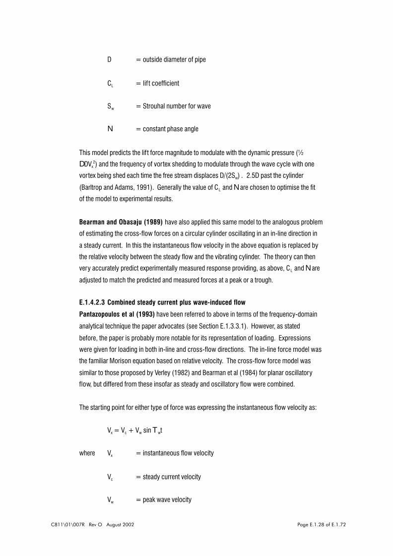
C811\01\007R Rev O August 2002 Page E.1.28 of E.1.72
D = outside diameter of pipe
CL = lif t coefficient
Sw = Strouhal number for wave
N = constant phase angle
This model predicts the lif t force magnitude to modulate with the dynamic pressure (½
DDVx2) and the frequency of vortex shedding to modulate through the wave cycle with one
vortex being shed each time the free stream displaces D/(2Sw) . 2.5D past the cylinder
(Barltrop and Adams, 1991). Generally the value of CL and N are chosen to optimise the fit
of the model to experimental results.
Bearman and Obasaju (1989) have also applied this same model to the analogous problem
of estimating the cross-flow forces on a circular cylinder oscillating in an in-line direction in
a steady current. In this the instantaneous flow velocity in the above equation is replaced by
the relative velocity between the steady flow and the vibrating cylinder. The theory can then
very accurately predict experimentally measured response providing, as above, CL and N are
adjusted to match the predicted and measured forces at a peak or a trough.
E.1.4.2.3 Combined steady current plus wave-induced flow
Pantazopoulos et al (1993) have been referred to above in terms of the frequency-domain
analytical technique the paper advocates (see Section E.1.3.3.1). However, as stated
before, the paper is probably more notable for its representation of loading. Expressions
were given for loading in both in-line and cross-flow directions. The in-line force model was
the familiar Morison equation based on relative velocity. The cross-flow force model was
similar to those proposed by Verley (1982) and Bearman et al (1984) for planar oscillatory
flow, but differed from these insofar as steady and oscillatory flow were combined.
The starting point for either type of force was expressing the instantaneous flow velocity as:
Vx = Vc + Vw sin Twt
where Vx = instantaneous flow velocity
Vc = steady current velocity
Vw = peak wave velocity
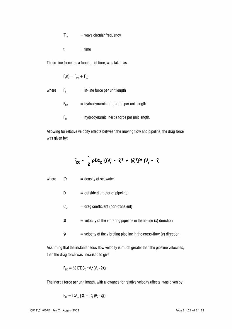
C811\01\007R Rev O August 2002 Page E.1.29 of E.1.72
Tw = wave circular frequency
t = time
The in-line force, as a function of time, was taken as:
Fx(t) = FDX + FIX
where Fx = in-line force per unit length
FDX = hydrodynamic drag force per unit length
FIX = hydrodynamic inertia force per unit length.
Allowing for relative velocity effects between the moving flow and pipeline, the drag force
was given by:
where D = density of seawater
D = outside diameter of pipeline
CD = drag coefficient (non-transient)
x0 = velocity of the vibrating pipeline in the in-line (x) direction
0y = velocity of the vibrating pipeline in the cross-flow (y) direction
Assuming that the instantaneous flow velocity is much greater than the pipeline velocities,
then the drag force was linearised to give:
FDX = ½ DDCD *Vx*(Vx - 2x0)
The inertia force per unit length, with allowance for relative velocity effects, was given by:
FIX = DAp {V0 x + CA (V0 x - (x)}

C811\01\007R Rev O August 2002 Page E.1.30 of E.1.72
where Ap = net cross-section area of the pipe
V0 x = instantaneous flow acceleration
(x = acceleration of vibrating pipe
CA = added mass coefficient (non-transient).
It is seen that the two components of the force equation contain coupling terms involving the
pipe motion (x0 and (x). The paper implies that these terms can be subsumed into the
equations of motion of the pipe as hydrodynamic damping and added mass effects. This
leaves the transient force equation as follows:
FX = ½ DDCD *Vx*/Vx + DAp(1+CA) V0 x
This is, in fact, the standard Morison equation using only the instantaneous flow velocity and
acceleration.
Similar arguments were applied to the cross-flow force, the equation for which appears as:
Fy = ½ DDCL (t) *Vx*(Vx - 2x0)
There are two key features of this equation that require further discussion: firstly, the
presence of the in-line pipe velocity in the definition of the cross-flow force; and, secondly,
the time-dependent lif t coefficient CL(t).
The presence of the in-line pipe velocity in the equation for the cross-flow force builds into
the analysis two complicating factors. Firstly, that motions of the pipeline in the in-line and
cross-flow directions are coupled; ie. in-line velocities affect cross-flow force and,
consequently, cross-flow motions. Secondly, the in-line velocity term is spatially as well as
temporally dependent; this would mean that unlike the in-line force given above, which is a
function of time alone and can therefore be regarded as a time dependent uniformly
distributed load, the cross-flow force per unit length varies not only with time but also along
the length of the pipeline. However, providing that the equations of motion of the pipe are
uncoupled, in principle, the in-line equations could be solved for x0 which could be inserted
into the Fy expression prior to solution of the cross-flow equation of motion.
The time-dependent lif t coefficient was given by:
CL(t) = CLM + CLO sin Tst
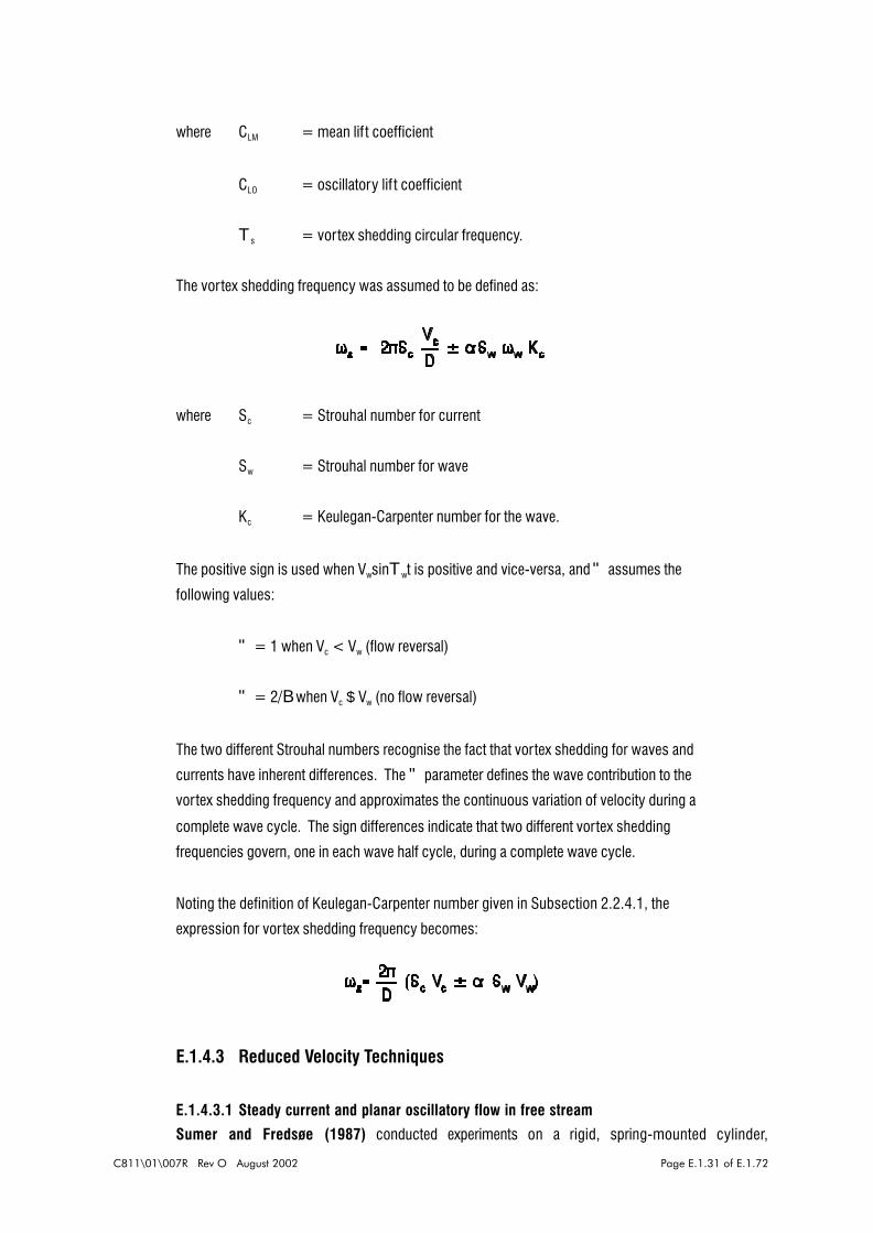
C811\01\007R Rev O August 2002 Page E.1.31 of E.1.72
where CLM = mean lif t coefficient
CLO = oscillatory lif t coefficient
Ts = vortex shedding circular frequency.
The vortex shedding frequency was assumed to be defined as:
where Sc = Strouhal number for current
Sw = Strouhal number for wave
Kc = Keulegan-Carpenter number for the wave.
The positive sign is used when VwsinTwt is positive and vice-versa, and " assumes the
following values:
" = 1 when Vc < Vw (flow reversal)
" = 2/B when Vc $ Vw (no flow reversal)
The two different Strouhal numbers recognise the fact that vortex shedding for waves and
currents have inherent differences. The " parameter defines the wave contribution to the
vortex shedding frequency and approximates the continuous variation of velocity during a
complete wave cycle. The sign differences indicate that two different vortex shedding
frequencies govern, one in each wave half cycle, during a complete wave cycle.
Noting the definition of Keulegan-Carpenter number given in Subsection 2.2.4.1, the
expression for vortex shedding frequency becomes:
E.1.4.3 Reduced Velocity Techniques
E.1.4.3.1 Steady current and planar oscillatory flow in free stream
Sumer and Fredsøe (1987) conducted experiments on a rigid, spring-mounted cylinder,
C811\01\007R Rev O August 2002 Page E.1.32 of E.1.72
principally in oscillating flow, but also with a limited number in steady flow. The spring suppor t
arrangements were such that the cylinder possessed a degree of kinematic freedom only in the
cross-flow direction. The effects on frequency response and vibration amplitude of Keulegan-
Carpenter number, Kc (peak flow velocity as a proportion of cylinder diameter times wave
frequency) and reduced velocity, Vr (peak flow velocity as a proportion of cylinder diameter
times cylinder natural frequency) were investigated. In addition to this, the roles played by
support spring stiffness and cylinder specific gravity were also examined briefly.
Results, in the form of graphs of various response frequency ratios, vibration amplitude ratios
and RMS cylinder displacement ratios, versus reduced velocity at fixed values of Kc were
presented. However, it should be noted that by fixing Kc in this way and varying Vr meant for
each Vr taken, a different wave frequency had to be imposed to maintain constant Kc . Thus, in
the graphs presented, the Vr axis represented not only var ying peak flow velocity but
concomitant wave frequency variation.
For Kc equal to 10 it was found that the frequency response of the cylinder modulated with the
wave frequency by exhibiting two vibrations per wave cycle across a range of reduced velocities
between two and ten. The response amplitude and RMS displacement each attained a single
sharp peak.
For an intermediate range of Kc numbers the frequency response of the cylinder depended on
the reduced velocity. At low Vr the number of response vibrations per wave cycle tended to be
around five times the Kc number (ie. the Strouhal frequency) and as the Vr number increased,
the number of response vibrations stepped down until two was reached, whereupon this value
was maintained for fur ther increases in reduced velocity. Within the ranges of reduced velocity
for which constant ratios of response frequency to wave frequency were found, individual peaks
of response amplitude and RMS displacement occurred. This gave a multi-peaked appearance
to the graphs of response amplitude versus reduced velocity over a range of reduced velocity,
which varied with Kc number. This was followed by a very much less sharp increase in
response amplitude with reduced velocity increased outside of this range. The height of the
peaks seemed to be allied closely to the oppor tunity for the response frequency to resonate with
the natural frequency.
For high Kc numbers these trends were repeated, but individual peaks in the response amplitude
curves become less distinctive, looking more like smooth curves. The propensity for the
response frequency to modulate at twice the wave frequency was always evident at high
reduced velocities, however, along with the maximum amplitudes of vibration tending to coincide
with resonance. The trend for high Kc numbers (eg. Kc = 100) was for the frequency response
to be very similar to that for steady current, ie. initial response at the Strouhal frequency
followed by lock-on to the natural frequency for an intermediate range of reduced velocity. The
C811\01\007R Rev O August 2002 Page E.1.33 of E.1.72
amplitude response was characterised by a sharp rise to a peak approximately at lock-on, but
the decay from the peak for increasing reduced velocity was much less steep in the case of
high K c number when compared with the steady flow case.
Interesting results were also obtained for Kc = 5. The response frequency was found to be
always equal to the wave frequency, indicating that the vibrations were caused by lif t force
variations. Moreover, self-excited vibrations with large amplitudes tended to occur at much
higher values of reduced velocity than was the case for the higher Kc numbers. These vibrations
could be initiated at reduced velocities similar in value to those corresponding to the high Kc
cases if a sufficiently large external disturbance was applied to the cylinder.
Regarding the effects of spring stiffness it was found that the two set-ups where the stiffness
of one was three times the other differed ver y little in terms of frequency response and
maximum amplitude of vibration. It appeared that lock-in occurred at systematically lower
reduced velocities in the case of the system with the stiffer spring than the softer spring; this
was attributed to the lighter damping in the stiff spring case.
It was also noted that the results obtained in the study reported in this paper were very similar
to corresponding ones in which a plane boundary was in proximity at a gap ratio of unity. The
authors concluded from this that no substantial change occurs in the response characteristics
of the cylinder when the gap ratio is increased from unity to infinity.
E.1.4.3.2 Steady current and plane boundary
Tsahalis and Jones (1981) have performed experiments on a flexible pipe in proximity to a
plane wall under steady flow conditions and investigated the effects of gap ratio on response
frequency and amplitude of vibration. The gap ratios studied were 50 (to represent free-stream
conditions), 6, 4, 3, 2 and 1. The end support conditions were simply-suppor ted with respect
to rotation, and full axial restraint, thus allowing some degree of membrane tension to develop
in cases of large vibration amplitudes.
In the case of the gap ratio of 50 the pipeline exhibited a frequency jump phenomenon. As the
flow velocity was increased, first perceptible vibrations occurred with the response frequency
close to the Strouhal frequency; with fur ther increases in flow velocity both the amplitude of
vibration and the response frequency increased (but the latter remained smaller than the
corresponding Strouhal frequency). This situation continued until at a particular reduced velocity
the amplitude of vibration peaked, and a fur ther increase in flow velocity resulted in a sudden
reduction in vibration amplitude, accompanied by a sudden increase in response frequency.
Further increase in flow velocity resulted in relatively constant amplitudes and frequency
responses. The authors suggest that this jump phenomenon is attributable to the nonlinearities
introduced into the bending rigidity of the pipe by the membrane tension, rendering the system

C811\01\007R Rev O August 2002 Page E.1.34 of E.1.72
similar in behaviour to a stiffening Duffing oscillator. This particular point highlighted the
potential problems of hydro-elastic dissimilarity in applying results from rigid, spring-mounted
cylinders to flexible pipelines.
The authors also highlight the dependence of response in terms of frequency and amplitude of
vibration on specific gravity of the pipe. As the specific gravity is lowered, critical reduced
velocity (the conditions of flow under which maximum vibration amplitude occurs) tends to
increase. Lower specific gravity would occur for a pipe in water as opposed to the same pipe
in air. The authors argue for a less limited definition of lock-in; rather than being defined as
response and vortex shedding frequencies coalescing into a single value close to the natural
frequency, the definition should be that the vibrating body "takes control" of the vortex shedding
in apparent violation of the Strouhal relationship.
A number of observations on the response of the pipe in the presence of a plane boundar y as
compared to that of the isolated (no boundary proximity) pipe, were made as follows:
! the increase of response frequency with flow velocity is less steep
! first perceptible vibrations take place at a higher reduced velocity
! the increase of vibration amplitude with flow velocity is less steep
! the maximum amplitude is attained at a higher reduced velocity
! the maximum amplitude is reduced
! once the maximum amplitude is attained it remains constant for higher flow velocities.
A direct consequence of this last point is that curves of vibration amplitude versus reduced
velocity tended to appear S-shaped rather than bell-shaped as for the isolated pipe.
All of these trends were exhibited by gap ratios decreasing from 6 to 2, as compared with 50,
but for a value of 1 they were reversed with the exception of the reduction of the maximum
amplitude. This appeared to be very nearly halved compared with the isolated case.
Fredsøe et al (1985) have conducted experiments on rigid, spring-supported cylinders exposed
to a steady current and possessing one degree of kinematic freedom by vir tue of a system of
spring supports in the cross-flow direct ion. Two spring stiffnesses were used: designated as
"soft" and "hard", and three sets of experiments per formed comprising the two spring types and
a cylinder specific gravity of one, and the soft spring combined with a cylinder specific gravity

C811\01\007R Rev O August 2002 Page E.1.35 of E.1.72
of 1.89. Gap ratios in the range zero to 1.7 were investigated.
Overall, the paper suggests that the vibrations are partly induced by vortex shedding and par tly
self-excitation (particularly in the case of very small gap ratios). In the latter case the vibrations
are caused by rapidly changing displacements which, because of the inability of the
downstream wake to adjust rapidly enough to accommodate the necessar y changes in fluid
discharge through the gap, lead to upward pressures on the cylinder when it is moving away
from the boundary. These types of vibration, however, may not occur spontaneously over a
range of flow velocities; in the experiments, perturbations in the form of an applied and then
released displacement, were necessary to instigate them.
Principal observations made from the experiments were as follows:
! the response frequencies were generally higher than the corresponding Strouhal
frequency except for reduced velocities less than 3 and greater than 8
! the response frequency increased with decreasing gap ratio
! there were no significant differences between results for the soft and hard spring
cases, except that there was a small tendency to larger frequencies in the stiff spring
case
! the cylinder specific gravity has some influence on the response frequency: at large
reduced velocities, the frequency decreases with increasing specific gravity; the
effect is more pronounced for small gap ratios
! the maximum amplitude of vibration occurred at larger values of reduced velocity as
the gap ratio was reduced
! the maximum amplitude of vibration increased as the gap ratio was reduced
! as the gap ratio was reduced from 1.7 down to 0.14 the curve of amplitude of vibration
versus reduced velocity tended to change from S-shaped to bell-shaped (similar to
what might be expected for an isolated pipe).
Large amplitude vibrations were only stimulated in the case of small gap ratios by artificially
introduced perturbations, as mentioned earlier. In general the size of perturbation (in the form
of initial displacement to diameter ratio) necessary to obtain vibrations depended upon gap ratio
and reduced velocity; for a given gap ratio the perturbation reduced linearly with increasing
reduced velocity, with a slope that reduced with reducing gap ratio. These relationships were
C811\01\007R Rev O August 2002 Page E.1.36 of E.1.72
such that threshold reduced velocities were determined at which no perturbations were required
to induce the self-excited vibrations. The threshold reduced velocities increased as the gap ratio
decreased and, for a fixed gap ratio were greater for the soft configuration than for the stiff one.
The differing vibration mechanisms in the case of a rigid cylinder in steady flow and in close
proximity to a plane boundary have also been investigated experimentally by Tørum and Anand
(1985). The cylinder in their case was fixed in the in-line direction and the main purpose of the
work reported in the paper was to investigate the effect of turbulence intensity on the mean drag
force and vibration amplitudes. Two sets of experiments were reported, referred to as Case 1
and Case 2, involving gap ratios of 0.5, 0.75, 1.0 and 3.0 for a turbulence intensity of 3%, and
a fixed gap ratio of 0.5 with turbulence intensities of 3.4, 5.5 and 9.5%. Turbulence intensity in
this case was defined as the ratio of the RMS velocity to the mean velocity. The experimental
set-up had an arrangement involving a dummy pipe (which moved above the free stream, in air,
in sympathy with the submerged cylinder) and a sand box which acted as an "impact preventer"
that restricted the gap to greater than about 10% of the cylinder diameter, thereby limiting the
motion of the cylinder.
For the Case 1 results, it was shown that the maximum value of mean drag coefficient was not
much affected by gap ratio; the magnitude of reduced velocity at which the maximum occurred
seemed to sh i f t to a higher value as the gap ratio reduced. Whilst reduction in gap ratio
appeared to reduce maximum amplitude of vibration, the responses for gap ratios of 0.75 and
0.5 were found to be amplified in the upward direction and asymmetric; the authors attributed
this to the possible existence of steady lif t due to flow constriction in the gap plus possible
vor tex shedding (see the account of Fredsøe et al (1985), earlier). In addition to this the
occurrence of the maximum amplitude of vibration shif ts to a higher reduced velocity as the gap
ratio decreases from 1.0 to 0.5.
For the Case 2 results, it was found that:
! the maximum amplitudes of vibration did not seem to be much affected by turbulence
intensity
! the occurrence of the maximum amplitude of vibration and subsequent amplitudes of
vibration at other levels shif ted to a lower reduced velocity at the turbulence intensity
of 9.5 compared with the lower values
! bottom proximity affects the lock-in range of the vibrating cylinder such that the vortex
shedding frequency did not lock-on to the natural frequency, but continued to increase
and control the cylinder motion; vibrations took place at the vortex shedding
frequency up to the maximum amplitude of vibration and differed only af ter the
C811\01\007R Rev O August 2002 Page E.1.37 of E.1.72
cessation of large amplitude vibrations.
E.1.4.3.3 Planar oscillatory flow and plane boundary
Sumer et al (1986) carried out experiments on a rigid, spring-mounted cylinder that was
restricted to cross-flow vibrations only. The flow conditions were principally wave-induced
currents, with Keulegan-Carpenter numbers in the range 10 to 100, but steady current results
were presented to allow comparison. A plane wall was also present in the experiments, with
gap ratios taken of 1.0, 0.4 and 0.15. The flow conditions were achieved by means of carriage
action in a water-filled flume. In the support arrangements for the cross-flow direction, two
types of springs were used: referred to as "sof t" and "stiff". Some additional experiments were
executed on the soft spring set-up but with a different cylinder mass, this allowed the effects
of changing specific gravity to be investigated. Except in the cases of steady current, the
reduced velocity was defined in terms of the maximum velocity (amplitude) of the wave motion,
the cylinder diameter and its natural frequency; the Keulegan-Carpenter number was defined
similarly but using the wave frequency. In the experiments, the reduced velocity was changed
by altering the peak velocity; in order to keep the Kc number constant for variable reduced
velocity it was necessar y, therefore, to change the wave frequency for each value of reduced
velocity.
In the case of a gap ratio of unity the following observations were made:
! For Kc = 10, the response frequency was twice the wave frequency (ie. the cylinder
underwent two oscillations per wave cycle) for reduced velocities in the range zero
to 10, following the Strouhal frequency. The amplitude versus reduced velocity curve
exhibited a sharp spike, maximising at around response and natural frequency
equality.
! For Kc = 20 and 40, the response frequencies were initially four and seven times the
corresponding wave frequencies, ie. corresponding fairly well with the Strouhal
frequency; however, with increasing reduced velocity the response frequencies
"jumped down" exhibiting ratios of 3 and 5 respectively; during these jumps, the
response frequencies reduced to being approximately equal to the cylinder natural
frequency. The amplitude versus reduced velocity curves exhibited two sharp spikes,
and the large amplitude regime extended over larger ranges of reduced velocity than
was the case at the lower value of Kc.
! For Kc > 60 (specifically = 100) the response frequency was initially 20 times the
wave frequency and corresponded with the Strouhal frequency; with increasing
reduced velocity, rather than the stepwise change in response frequency exhibited by
the lower Keulegan-Carpenter numbers, there was a gradual reduction in response

C811\01\007R Rev O August 2002 Page E.1.38 of E.1.72
frequency to 10 times the wave frequency. The response frequency during this
gradual change, was maintained roughly at the cylinder natural frequency. The
amplitude versus reduced velocity curve rose very rapidly af ter onset of vibrations,
before maximising when the response frequency equalled the cylinder natural
frequency; thereaf ter, the amplitude remained at the maximum value over the full
range of reduced velocity tested.
! For the steady current case the response frequencies followed the Strouhal frequency
before a lock-on condition was attained for a short range of reduced velocity;
thereaf ter, response frequency corresponded to values less than the Strouhal
frequency. The amplitude versus reduced velocity curve rose very steeply in the
range of reduced velocity leading up to lock-in, peaked during lock-in, before reducing
more gradually for further increases in reduced velocity
! the response frequencies were found to correspond very closely with the vortex-
shedding frequencies of fixed rigid cylinders in a free stream (ie. a cylinder held
stationary with no boundary in proximity)
! in comparing the sof t and stiff spring results it was found that there was little
difference between the response frequencies for the two cases; however, the vibration
amplitudes for the stiff spring cases tended to be generally larger and this was
ascribed to the lighter damping in that case
! the maximum amplitude for Kc = 10 was very close to that pertaining to the current
case and, generally, the effect of increasing Kc was to reduce the maximum amplitude
(by a factor of two for a change in Kc from 10 to 100)
! the initiation of vibration of the cylinder under wave-induced current generally occurred
at smaller reduced velocities than for steady current; this was attributed to the fact
that the reversal of wake may create flow velocities larger than the free stream
velocity.
In the case of gap ratios of 0.15 and 0.4, the following observations were made:
! for small values of reduced velocity, and for all of the Keulegan-Carpenter numbers
tested, the mean gap ratio was maintained at the equilibrium value in still water, ie.
there was no overall lif t of the cylinder
! as the reduced velocity was increased, however, the mean gap ratio increased,
indicating that (on average) the cylinder was repelled away from the boundary; also,

C811\01\007R Rev O August 2002 Page E.1.39 of E.1.72
the smaller the Kc number, the larger the mean gap ratio; thus, the overall li f t force on
the cylinder increased with increasing reduced velocity, but decreased with increasing
Keulegan-Carpenter number.
The following conclusions were drawn from the experiments involving the gap ratios of 0.15 and
0.4 concerning the frequency response and vibration amplitude of the cylinder:
! the response frequencies generally did not follow the vortex shedding frequencies
! the vibration amplitudes increased significantly as the gap ratio decreased (the
converse of this occurred for the steady current case, the maximum amplitudes were
very similar in value for gap ratios of 0.15 and 0.4)
! the curves of amplitude of vibration versus reduced velocity in the cases of the gap
ratios less than one were "S"-shaped rather than "peaked" as was the case for a gap
ratio of unity
! the vibration amplitudes were significantly reduced at times when the wave velocity
passed through its zero crossing points
! the mechanism of vibration differed depending on gap ratio; for the gap ratio of 0.15
the cylinder experiences a lif t force mechanism that stems from wall proximity effects
! incipient vibration appeared to occur at values of reduced velocity that were smaller
in the case of waves than in the case of currents for small values of Keulegan-
Carpenter numbers only (10, 20); this earlier initiation was attributed to the larger lif t
forces present for the smaller Kc numbers.
As mentioned above, a number of tests were carried out to investigate the effects increased
cylinder specific gravity (increased mass) had on the response characteristics. It has to be
borne in mind that an increase in mass will also increase the reduced damping or stability
parameter. The specific gravity was, in fact, changed from 1.0 to 1.72 and experiments
undertaken for steady current and wave-induced flow with a Kc number of 40. The following
observations were made:
! In the case of steady current, it was found that the increase in specific gravity:
- reduced the maximum amplitude of vibration significantly, and increased the
reduced velocity at which large amplitude vibrations were induced in the
case of a gap ratio of unity

C811\01\007R Rev O August 2002 Page E.1.40 of E.1.72
- had negligible effects on the vibration amplitude versus reduced velocity
curve in the case of a gap ratio of 0.4.
- changed the amplitude versus reduced velocity curve from S-shaped to
continuously rising with increasing reduced velocity in the case of a gap
ratio of 0.15 (this meant that the magnitudes of the vibration amplitudes
were not limited)
! In the case of wave-induced flow with a Keulegan-Carpenter number of 40, it was
found that the increase in specific gravity
- reduced the maximum amplitude of vibration most significantly for a gap
ratio of unity; smaller reductions were evident at the smaller gap ratios
- the onset value of reduced velocity was increased most significantly for a
gap ratio of unity; the increases became progressively smaller as the gap
ratio decreased.
Although no direct investigation of vortex shedding was made, the indications from the work
were that vibration of the cylinder was by vor tex shedding in the cases of a gap ratio of unity.
For the gap ratio of 0.15, wall proximity/lif t force effects were the main mechanism of vibration
of the cylinder. For the intermediate gap ratio of 0.4, a combination of these two influences was
responsible for the vibration.
E.1.4.3.4 Steady current, planar oscillatory flow and plane boundary
Tsahalis (1984) investigated the vortex-induced vibrations of a flexible cylinder near a plane
boundary exposed to steady current and wave flow. The cylinder had a length:diameter ratio
of 113:1; it was simply-supported with respect to bending moment in both the in-line and
cross-flow directions, but fixed in the axial direction. Despite this the pipe natural frequencies
were the same in the in-line and cross-flow directions, indicating negligible membrane tension
due to sag. The response of the model to vor tex-induced vibrations was determined for a wide
range of values of gap ratio and Keulegan-Carpenter number. In the paper, however, results only
for gap ratios of infinity and unity in combination wi th Kc numbers of 0 (steady current) and 20
were presented. In all tests the wave frequency was kept constant and the Kc variation was
achieved by varying the wave height.
In the case of steady flow and an infinite gap ratio it was found that the first perceptible cross-
flow vibrations took place at a reduced velocity of 3 with a response frequency close to the
Strouhal frequency, and a maximum amplitude occurred at a reduced velocity of about 7 with
a frequency of about 0.92 of the natural frequency. In-line response was the same in character,
but with the exceptions that the frequency was twice that of the cross-flow vibration and the

C811\01\007R Rev O August 2002 Page E.1.41 of E.1.72
amplitude was one-quarter of the cross-flow amplitude. These results were much as expected,
and indicated that, in displacement terms, the pipe underwent a figure-of-eight type motion.
For the situation of a gap ratio of unity, and under steady flow conditions, the response in the
cross-flow direction was similar to that for the corresponding case of a flexibly-mounted rigid
cylinder (Tsahalis and Jones, 1981). The proximity of the plane boundary had the following
effects on the cross-flow response compared with the isolated pipe:
! the maximum single amplitude was reduced by a factor of two and persisted over a
wider range of reduced velocity
! the first perceptible vibrations took place at a higher reduced velocity.
In the case of the in-line direction the response was similarly affected, however, the response
frequencies were found to be equal to those in the cross-flow direction. This suggests that,
while the vibrations are induced by vortex shedding, the wake and interaction between the wake
and the vibrating pipe are influenced by the presence of the plane boundary and it appeared that
the pipe underwent oval-shaped (rather than figure-of-eight) motion.
In the case of combined steady and wave-induced flow on the pipe with an infinite gap ratio it
was found that the major effect of superimposed flow was to give rise to vor tex-induced
vibration over the whole range of reduced velocity. Specifically in the cross-flow direction it was
found that in comparison with the steady flow case:
! the single amplitude was larger for reduced velocity less than 6
! the maximum single amplitude was reduced in value, but still occurred at a reduced
velocity of 7
! the single amplitude was smaller for reduced velocities greater than 7
! the dominant response frequencies were the same as in the steady flow case, except
for reduced velocity greater than nine, where they become larger.
In the in-line direction, it was found that:
! the single amplitude was larger for all reduced velocities
! the maximum single amplitude was increased by 50% and it persisted over a wider
range of reduced velocity
C811\01\007R Rev O August 2002 Page E.1.42 of E.1.72
! the dominant response frequencies change dramatically and follow closely the
dominant response frequencies in the cross-flow direction, except for reduced velocity
greater than 8 where they become larger.
It was also found that in addition to the dominant frequency of vibration in the in-line and cross-
flow directions, additional neighbouring frequencies (with energy contents of at least 10% of the
dominant) were present, indicating that the pipe did not undergo pure harmonic vibrations.
For the final situation of the pipe exposed to combined steady and wave-induced flow and a gap
ratio of unity it was found that the flow regime, in combination with the boundary proximity, had
a tremendous effect of the vortex induced vibration of the pipe. The flow regime was such that
for reduced velocities in excess of 2.3 the flow did not reverse; ie. the current velocity always
exceeded the amplitude of the wave velocity.
In comparison with the steady flow free-stream conditions (no boundary proximity) it was found
that in the cross-flow direction:
! the maximum of the single amplitude was reduced by a factor of about three
! the maximum persisted over almost the whole range of reduced velocity tested (this
had the effect of "flattening" the amplitude versus reduced velocity graph, making it
less "peaky")
! the dominant response frequencies were larger, but their trend remained unchanged.
In the in-line direction, it was found that:
! the maximum of the single amplitude was reduced by a factor of around two
! the maximum persisted over almost the whole range of reduced velocity tested
! the dominant response frequencies followed the trend of their counterparts in the
cross-flow direction.
The frequency content of the responses in both the in-line and cross-flow directions
indicated that the pipe did not undergo pure harmonic vibrations.
Tsahalis (1985) also reported an extension to the series of tests summarised above, in which
steady currents were superimposed with wave-induced currents corresponding to Keulegan-
Carpenter numbers of 0, 5, 10, 15, 20, 25 and 30, along with proximities to a boundary with gap
C811\01\007R Rev O August 2002 Page E.1.43 of E.1.72
ratios of 1, 2, 4, 6 and 4. The test conditions were as described above.
In the case of steady current and regular waves where the gap ratio was held constant and
Keulegan-Carpenter number was varied, it was found that:
! in the cross-flow direction
- the maximum amplitude of vibration generally decreased with increasing Kc
- the first perceptible vibrations took place at smaller reduced velocities as
Kc increased
- vibration frequencies remained basically unchanged
! in the in-line direction
- the maximum amplitude of vibration generally increased with increasing
Kc
- the first perceptible vibrations took place at smaller reduced velocities for
increasing Kc
- frequencies of vibration remained basically unchanged.
For the situation of steady current and regular waves in which the Keulegan-Carpenter
number was held constant and the gap ratio was varied, it was found that for both cross-
flow and in-line directions
! the maximum amplitude of vibration decreased slightly with decreasing gap ratios in
the range 2 to 4; however, it decreased dramatically for a fur ther reduction in gap ratio
to unity.
! The frequencies of vibration remained basically unchanged.
Jacobsen et al (1984) carried out tests on an elastically-supported cylinder in proximity to a
plane rigid boundary in flows stemming from steady current, waves and waves superimposed
on steady current. Some results from an irregular wave train are also reported. The cylinder
appeared to be allowed degrees of freedom in the in-line and cross-flow direction, although in
the paper, only the results of the analysis of the displacements (in terms of maxima and RMS
values) in the cross-flow direction are included. Gap ratios of zero (cylinder just touching the
plane boundary in its equilibrium state), 1.0 and 0.5 were tested. In presenting results, the
wave conditions were characterised by the Keulegan-Carpenter number and the reduced velocity

C811\01\007R Rev O August 2002 Page E.1.44 of E.1.72
based on the maximum oscillatory velocity. The combined wave and current experiments were
performed at steady flow velocities of 0.2 m/s and 0.6 m/s, the reduced velocities for these
were expressed in terms of the wave parameters. For the waves, Keulegan-Carpenter numbers
of 30, 60, 90 and 120 were investigated.
It was found that in comparing the results for steady current with those for waves:
! for a gap ratio of unity, and in steady current, peak maximum oscillations occurred
between reduced velocities of 5 and 6 and af ter passing through a second lower
plateau, movements almost ceased for Vr above about 9; in the case of the wave
motion, the vibration amplitudes were significantly less than the steady current case
in the resonance range, but were larger at the low and high range of reduced
velocities; maximum and maximum RMS amplitudes appeared to reduce with
increasing Kc numbers
! for a gap ratio of 0.5 unsymmetrical responses occurred, owing to the close proximity
of the boundary; instead of the typical "bell"-shaped maximum amplitude versus
reduced velocity curve obtained for the steady current, the curve for wave flows was
more S-shaped with a peak similar in value to that of the current which was
independent of Keulegan-Carpenter number; similar traits were displayed by the
corresponding RMS amplitude curves
! for a gap ratio of zero the forcing mechanism changed and was judged to be not
related to the regular shedding of vor tices; it was found that the response amplitudes
almost increased continuously with increasing reduced velocity regardless of
Keulegan-Carpenter number; moreover, the amplitudes increase for decreasing Kc
numbers for Vr below 5, meaning that the excitation force is larger and stems from a
lif t away from the boundary.
For steady current superimposed on wave compared with steady current, it was found that:
! for a gap ratio of unity, significant changes in curves of RMS amplitude versus
reduced velocity occurred for both current velocity cases; larger amplitudes of
vibration were found for the current velocity of 0.2 m/s for almost all reduced
velocities; for the 0.6 m/s curren t velocity radical changes were introduced into the
response curves, the maximum values of RMS amplitude disappeared giving more
constant values over the range of reduced velocities investigated
! for a gap ratio of 0.5, the response curves for a current velocity of 0.2 m/s were found
to be very similar to the steady current ones, regardless of the Keulegan-Carpenter
C811\01\007R Rev O August 2002 Page E.1.45 of E.1.72
number; the application of the 0.6 m/s current had a similar effect to the one found
for a gap ratio of unity.
Some of the most revealing results, in phenomenological terms, however, stem from the
displacement time series given in this paper. In the case of regular waves, it was shown that
vibration amplitudes vary within each half-wave period and that the variation depends on
reduced velocity: vibrations almost decay to zero for small Vr, whereas for large V r vibrations
were sustained. Similar patterns were displayed by results from flow conditions of regular wave
combined with steady current, and irregular waves. Thus "pulses" of high frequency vibration
resulted, that modulated to half periods of velocity variation during which the reduced velocity
was of sufficient value to cause resonance. In the case of irregular waves particularly this
meant that it was feasible for long periods to elapse without any vibrations, but vibrations could
build up and decay during the passage of a large wave.
The distributions of response double amplitudes also showed ver y interesting features. For the
regular wave example given (which corresponded to a Keulegan-Carpenter number of 90) over
the range of reduced velocity taken (3.8 to 6.5) there was little difference between the value of
the peak amplitudes; the distribution changed quite radically however as reduced velocity was
altered from 3.8 to 6.5, from having the major par t of the amplitudes concentrated at small
values to being concentrated at larger values.
Response to irregular waves is, by definition, a complex phenomenon. The authors suggest in
this paper an ingenious way of dealing with irregular waves by first dividing the time series up
into a sequence of single oscillations (by means of a zero up-crossing analysis) each described
by a period and maximum velocity. These, in turn define a Keulegan-Carpenter number and
reduced velocity for that oscillation. The corresponding vibrations are then computed from the
regular wave test results assuming that each irregular oscillation contributes to the total
vibrations as one regular wave with identical parameters. An example amplitude distribution
computed in this way was compared with a measured result, and the correlation was found to
be ver y good, but it tended to underpredict the number of small amplitudes and overpredict the
number of large amplitudes. This was because the use of the regular wave did not include the
build-up and decay of amplitudes, but used the maximum; this tended to overemphasise the
larger amplitudes at the expenses of the smaller ones. Nevertheless this method showed great
promise in terms of adaptation to fatigue analysis.
Bryndum et al (1989) carried out a large number of tests in both a flume and a towing tank.
Two types of model were tested: a short segment of pipe (essentially a rigid cylinder) that was
spring-mounted in such a way to allow displacements in the in-line and cross-flow directions;
a long flexible pipe suspended between low-friction hinges which gave simple-support for out-
of-straight bending. A flat plate was put in proximity to the models to represent the seabed.
In both model types the following flow types were used:

C811\01\007R Rev O August 2002 Page E.1.46 of E.1.72
1. Steady current
2. Regular waves
3. Combined steady current and regular waves
4. Irregular waves
5. Combined steady current and irregular waves
and the effects of reduced velocity, Keulegan-Carpenter number and current ratio (ratio of
current and maximum wave velocity in the case of combined flow) were investigated.
In the specific case of the rigid pipe tests, a total number of 2550 individual experiments were
performed covering the variation of a wide range of parameters: gap ratio, roughness ratio,
stability parameter, turbulence intensity, presence of scour or relative scour hole depth. In
addition, tests with no (fixed) or one degree-of-freedom, or in transient conditions, or with
different specific masses were carried out.
In the specific case of the flexible pipe tests, a total number of 240 individual experiments were
carried out covering the effects of: incident angle of f low, pipe length to diameter ratio, effective
axial stiffness at the supports, pipe tension and gap ratio.
For the rigid pipe tests under steady current it was found that:
! the gap ratio imposed geometrical limitations on pipe displacements; for small gaps
(ratio < 0.4) impact energy absorption occurred and regular vortex shedding did not
take place, with pipe motions initiated by fluctuating hydrodynamic lif t; for large gaps
(ratio > 0.8) vortex shedding occurred with the response resembling that of a cylinder
in a free stream
! the effects of increased stability parameter (damping) were to reduce displacements
at resonance in the cases of large gap ratio.
For the rigid pipe tests under regular wave conditions it was found that:
! in a reference test with a Keulegan-Carpenter number of 10 and a gap ratio of 0.8, the
converse of what normally happens in steady flow occurred in that the in-line vibration
amplitudes were potentially much larger than the cross-flow ones; moreover, the in-
line amplitude versus reduced velocity curve increased monotonically with increasing

C811\01\007R Rev O August 2002 Page E.1.47 of E.1.72
reduced velocity and did not exhibit a maximum
! the response was highly dependent on the Keulegan-Carpenter number; for a small
Kc of 5 resonance with the wave frequency was possible at suitable reduced
velocities, thus giving the in-line amplitude versus reduced velocity curve a local peak;
this effect disappeared with increased Kc number where the response curve reverted
to a monotonic form, but the rate of increase with reduced velocity diminished with
increasing Keulegan-Carpenter number
! the cross-flow amplitudes were generally much lower than the in-line ones; the cross-
flow amplitude versus reduced velocity curves occasionally displayed local peaks
which are associated with shif ts in the number of cylinder oscillations per wave period
! the effect on the in-line vibrations of reducing the gap ratio was not very significant;
in the cross-flow direction, however, amplitudes of vibration increased with reducing
gap ratio owing to the lif t force effects referred to earlier
! the effects of increased damping were negligible, owing to the relative magnitudes of
the damping and resonance forces
! the introduction of combined steady current had little effect on the cross-flow
response over a range of current ratios between zero and 2; steady current appeared
to reduce the vibration amplitudes compared to the pure wave case with reductions
becoming greater as the current ratio increased.
For steady flow tests on the flexible pipe there were found to be some differences between the
responses of the flexible pipe and the rigid cylinder. Significant vibrations for the flexible pipe
did not occur until larger reduced velocities than those necessary for the rigid cylinder;
moreover, relatively high in-line responses were observed in the case of the pipe, that were
absent for the cylinder. The authors ascribe these differences to the fact that, for the long
flexible pipe, the fundamental frequencies in the in-line and cross-flow directions were different.
In those cases of steady flow it was found that the effect of pipe tension was quite profound.
Increased pipe tension tended to increase the amplitudes of vibration very significantly in both
the cross-flow and in-line directions.
For the flexible pipe subjected to regular wave flow it was found that the measured response
was independent of the wave incident angle within the range zero to 45 degrees.
C811\01\007R Rev O August 2002 Page E.1.48 of E.1.72
E.1.4.3.5 Steady current and scour trenches
Sumer, Mao and Fredsøe (1988) conducted an experimental investigation of the effects of the
proximity of a scour trench on the vibration characteristics of a rigid cylinder in steady flow. The
cylinder was spring-supported in the cross-flow direction and held fixed in the in-line direction.
The scour holes used in the experiments were produced with the cylinder held fixed against
motion and sitting on an erodible bed comprising a sediment with d50 = 0.36mm and %(d85/d15)
= 1.4 (d is the particle diameter) and allowing a steady flow to pass for 30 minutes. In
conducting a vibration test the cylinder was freed in the cross-flow direction and the test then
performed in a typical sequence; the scour profile remained vir tually unchanged during this.
Three gap ratios (relative to the line of the undisturbed bed) were tested: 0.9, 0 and -0.3. The
paper is not clear over the depth of the scour trench, but indications were that it was of the
order of 0.6 times the cylinder diameter. Data are given in the paper in terms of frequency and
double amplitude.
It was found that:
! the amplitude and frequency responses did not resemble those of a cylinder placed
near a plane boundary; instead of S-shaped amplitude response curves (plane
boundary), the curve for gap ratios of zero and -0.3 were bell-shaped; response
frequencies were lower than in the case of plane boundary experiments
! the response behaviour was found to be quite similar to that obser ved for boundary-
free cylinders where vortex shedding is the only agent responsible for the vibrations;
flow visualisation revealed that vor tex shedding was present for every gap ratio tested
! the range of reduced velocity within which appreciable vibration amplitudes occurred
changed significantly with gap ratio, even though the maximum amplitude experienced
remained unchanged
! incipient vibrations started relatively early for larger gaps
! the value of reduced velocity at which the maximum vibrations occurred increased as
the gap ratio decreased
! the responses of cylinders with gap ratios of 0.9 and infinity were vir tually identical.
E.1.4.3.6 Planar oscillatory flow and scour trenches
In a series of papers Sumer et al (1988, 1989) have studied experimentally the vibrational
response of rigid, elastically-supported cylinders to wave-induced fluid motion and in proximity
to an idealised scour trench. Both regular (sinusoidal) and irregular waves were modelled at
C811\01\007R Rev O August 2002 Page E.1.49 of E.1.72
Keulegan-Carpenter numbers of 10 and 40, along with gap to diameter ratios ranging from -0.8
to 2 (where a negative number indicates immersion of the cylinder within the scour trench).
Reduced velocities were taken in the range 3-8, with the definition of Vr related to the amplitude
of velocity in the regular wave case, and the significant velocity amplitude in the case of
irregular waves.
They noted that for cross-flow vibrations in regular waves, and for Kc = 10, the frequency of
vibration was always maintained at twice the wave frequency across the gap ratio and reduced
velocity ranges tested. Moreover, the number of in-line vibrations per wave cycle was one more
than the number of cross-flow vibrations, ie. three.
It was found that amplitudes of vibration in the cross-flow direction increase as Vr increased,
attaining their peak values when the frequency of vibration and the natural frequency
approximately coincide in value. At high negative gap ratios (-0.5, -0.8) amplitudes of vibration
tended to become limited by impact of the cylinder with the sidewalls of the scour trench. Two
kinds of in-line motion of the cylinder were evident: those modulated with the wave frequency,
and superimposed higher frequency motions modulated with the vortex shedding (when it
occurred). Peaks of vibration amplitude in the in-line direction tended to be when the frequency
of vibration was approximately half the natural frequency.
An alternative pattern of response was exhibited by the cylinder for flow regimes corresponding
to Kc = 40 in regular waves. The cross-flow response depended upon the gap ratio: for gap
ratio positive the cross-flow frequency of vibration was 10-11 times the wave frequency at small
values of reduced velocity, with this factor reducing as Vr increased (the vibrations were due
to vortex shedding); for gap ratios between zero and -0.5, the vortex shedding was suppressed
owing to trench wall proximity and flow blockage, and the cylinder experienced a cross-flow
force oscillating at twice the wave frequency (cf. Kc = 10), thus the frequency of vibration is
twice the wave frequency; with gap ratios between -0.5 and -0.8 the vortex shedding
reappeared, and the frequency of vibration followed the same kind of variation as was the case
for a positive gap ratio, although peak amplitudes of vibration were somewhat smaller. Overall
in-line vibration amplitudes tended to be distinctly smaller for Kc = 40 than for Kc = 10.
In general terms it was found that for regular waves, and comparing the results for scour trench
with those for flat seabed proximity:
! when the gap ratio was two-diameters there was little difference between the two
sets of results
! when the cylinder is placed in a scour trench the amplitudes and frequencies of
vibration (for a given reduced velocity) are greatly reduced compared with those
C811\01\007R Rev O August 2002 Page E.1.50 of E.1.72
corresponding to a flat bed.
For irregular waves, and Kc = 10, the cross-flow vibrations depended on the gap ratio. For a
positive gap ratio the vibrations were driven by vortex shedding; lock-in occurred and the cylinder
simply started to vibrate at its natural frequency when the vortex shedding frequency coincided
with this. For negative gap ratios the vortex shedding was suppressed and the cylinder was
subjected to a cross-flow force oscillating at twice the wave frequency. The maximum
amplitudes of cross-flow vibrations were, in general, greater than the corresponding values for
regular waves. The in-line vibration responses were vir tually indistinguishable from those
obtained from the regular waves and, in overall terms, the above response was the same for
conditions where Kc = 40.
The authors of these two papers draw the following conclusions:
1. The position of the cylinder relative to the trench is an important determining factor for
the vibratory response of the cylinder.
2. For a cylinder exposed to irregular waves, the pattern of frequency response appears
to be the same as in regular waves when the gap ratio is negative. The cross-flow
vibration amplitudes are generally larger for irregular waves. The same is also true for
the in-line movements of the cylinder.
3. The response of a cylinder placed in a trench is markedly different from that near a
flat boundary. The amplitudes of vibration are greatly reduced when the cylinder is
placed in a trench. The cross-flow frequencies are also reduced.
E.1.4.4 General Fatigue Calculations for Pipeline SpansTsahalis and Jones (1982) have made fatigue life calculations for pipeline spans exposed to
steady flow and undergoing vor tex-induced vibrations. The effect of the proximity of the bed
was taken into account by utilising the results of model tests. They used a very simple
structural model involving a simply-supported beam to estimate strain ranges corresponding to
a single mode of vibration. A formula for fatigue life in years was developed that is a function
of a number of normalised parameters, including span length over outside diameter, steel pipe
diameter over outside diameter, vortex shedding frequency over span natural frequency, and
vibration amplitude over outside diameter. Fatigue lives were calculated over a twelve-hour tidal
cycle using what amounted to a reduced velocity technique (see Section 2.4.3 above). In this,
graphical results from experiments on a flexible pipe were used to estimate vortex shedding
frequency and amplitude ratios for different proximities between pipeline and seabed, and
different span lengths. It was shown that fatigue life was extremely sensitive to span length
(increases in span length reduced fatigue life or conversely increased fatigue damage). Most
C811\01\007R Rev O August 2002 Page E.1.51 of E.1.72
interestingly, curves of fatigue life versus span length exhibited minimum fatigue lives (around
0.2 to 0.3 years) for finite ratios of gap beneath span to pipeline outside diameter.
Rather curiously, the calculations of Orgill et all (1990) indicated the opposite to the above,
namely that fatigue damage reduced (and hence fatigue life increased) with increasing span
length. They used an equivalent lumped parameter system obtained by considering only the
mode of vibration corresponding to the lowest frequency of vibration in the cross-flow direction
along with an equation of motion involving a time-dependent force modulated at the vortex
shedding frequency. Idealised fatigue damage was taken as a stress range raised to a power.
Expressions were developed to relate the response of a prototype span to that of a simpler
experimental model (rigid elastically-suppor ted cylinders, for example) by means of the ratio of
various key non-dimensionalised parameters.
For the purposes of parametric studies, however, model parameters were set to unity and mode
shapes corresponding to assumed conditions of simple support and clamped ends were taken.
Parametric evaluations were made of the effects of mode shape, span length, axial load and
damping on fatigue damage, all of which (unsurprisingly) were shown to be important in fatigue
calculations. As mentioned earlier, the results indicated (rather perversely) reductions in fatigue
damage with increasing span length (this would only be the case if membrane tension were
allowed to participate at longer span lengths thereby leading to possible reductions in stress
ranges, an effect not present in their model). The effects of fixed value axial load were
investigated, and it was found that increasing tension resulted in very little change to fatigue
damage (probably for reasons outlined above); curiously, for the simply supported spans,
compressive axial forces caused reductions in fatigue damage. As might be expected, damping
tended to reduce fatigue damage.
Tsahalis (1983) extended the ideas developed in Tsahalis and Jones (1982) into the concept
of "generalised" fatigue damage. This is based on the fact that, excluding geometric parameters
such as outside diameter, pipe diameter, span length and natural frequency of vibration, fatigue
damage is a function of the ratios of response frequency to natural frequency and vibration
amplitude to pipe diameter. By dividing out the geometric parameters and a time period over
which a particular flow velocity is sustained, a generalised damage parameter results which is
a function of response frequency ratio and amplitude ratio. From experimental data these ratios
are available (in principle, if not in fact) as functions of reduced velocity and, say, gap ratio
between pipe and seabed. Such data then allows the generation of a generic graph of
generalised fatigue damage versus reduced velocity for different values of gap ratio from which
damage can be determined for a given flow condition. Multiplication of this by the normalisation
factors and the period over which the flow condition occurs gives the fatigue damage.
Repetition of this for all flow regimes and periods of interest, summing the damages and taking
the inverse yields the fatigue life.
C811\01\007R Rev O August 2002 Page E.1.52 of E.1.72
E.1.4.5 Summary of Literature in Relation to Assessment IssuesAt this stage it is worth summarising the literature covered in Subsection E.12.4, par ticularly that
contained in E.2.4.3 and concerned with, in effect, reduced velocity techniques. There is a
tremendous amount of detail in the reviews presented, and a technical summary would be part
of the process of forming a database that can be quantitatively interrogated. The building of this
database is judged to be outwith the scope of the present work and is proposed as a
recommended piece of work in Section E.4. For the present purposes, therefore, the summary
is confined to the relationship between the literature reviewed and the important issues in
dynamic response of pipeline spans raised in Subsection E.1.4.1 and illustrated in Figure E.1.12.
The summary addresses whether the literature covers the ground in terms of the issues
identified earlier and, therefore, contributes to an assessment of the feasibility of any database
derived from the literature. The summary is presented in Figure E.1.13; this comprises a matrix
made up from combinations of flow conditions, cylinder type and seabed effects; degrees of
kinematic freedom are indicated as superscripts on the entries in the matrix.
It can be seen that the majority of information is related to rigid cylinder experimentation, with
the minority covering flexible cylinders or quasi-pipelines. In the case of rigid cylinders, most
seabed effects are well covered, but it would appear that there is insufficient information on
scour trenches in amalgamation with combined steady current and wave flow conditions. For
flexible cylinders in combination with a plane boundary, it is seen that all flow conditions are
reasonably well-covered, but there is an absence of information connected with free stream
conditions and scour trenches. The lack of free stream flow conditions information is not seen
as a serious shortfall because many of the references involving the influence of a plane
boundary generally include, in effect, free stream conditions at sufficiently large gap ratios.
All-in-all there is probably sufficient literature of enough quality to cover the main aspects of
many practical problems of pipeline span assessment by reduced velocity techniques. This
would be able to provide a body of information to form a database that would represent a
significant advance over the limited information currently held in codes of practice and design
guidelines (eg DNV, 1981).

C811\01\007R Rev O August 2002 Page E.1.53 of E.1.72
E.1.5 FATIGUE LIFE AND DAMAGE CALCULATION
E.1.5.1 Limits Set by Codes and GuidelinesThree codes were considered in this respect; these are as follows:
! BS 8010 : Part 3 : 1993
Code of Practice for Pipelines Subsea: design, construction and installation
! Det Norske Veritas (DNV) : 1981 (reprint with corrections 1982)
Rules for Submarine Pipeline Systems
! Institute of Petroleum, 4 edition, 1982
Pipeline Safety Code (IP6)
These documents contain various degrees of guidance, although none were deemed to be
comprehensive.
E.1.5.1.1 BS 8010
BS 8010 is very specific regarding strain-based design. Clause 4.2.7.1: use of allowable
strain in design, states that:
"...This approach is only permissible where geometric considerations limit the maximum strain
to which the pipeline can be subjected and where the controlled strain is not of a cyclic or
repeated nature".
This would appear very definitively to rule out the application of strain-based approaches to
fatigue calculations.
For actual fatigue calculations, Clause 4.2.8 applies; two sub-clauses follow, dealing with
fatigue loads and fatigue life.
Clause 4.2.8.1 covers fatigue loads stating that all fluctuating loads should be considered in
establishing the effect of fatigue on the pipeline, except those that produce stresses below
the threshold for fatigue damage. Many S-N curves for welded tubulars, however, do not
incorporate a threshold. Typical sources of fluctuating loads are suggested to include:
! wave forces
! vibrations caused by vortex shedding, product flow, or other phenomena
! operation cycles

C811\01\007R Rev O August 2002 Page E.1.54 of E.1.72
! alternating movement of platforms and other structures
Clause 4.2.8.2 covers fatigue life. A general statement is given first that consideration
should be given to the fatigue life of pipelines to ensure that minor defects do not grow to a
critical size under the influence of cyclic loading. The code gives multiplying factors
corresponding to fixed ranges of stress variations which are applied to the number of daily
stress cycles occurring for the principal stresses within the ranges. The total sum of
factored and unfactored cycles should not exceed 15000. This simplistic approach is
suggested as an alternative to more comprehensive fatigue analyses based on fracture
mechanics or S-N curve approaches.
Spanning pipelines are dealt with under Clause 4.6, with vortex shedding and fatigue covered
by 4.6.4. The clause states specifically that:
"Pipeline ... oscillations induced by internal or external fluid flow should be considered".
The pipeline design should either prevent pipeline oscillations, or show that if they occur
they are acceptable with respect to the following:
! service considerations
! strength
! fatigue
! coating integrity.
As most of the loads contributing to fatigue are of a random nature, statistical considerations
will normally be required for determination of the long-term distribution of fatigue loading
effects. The code allows the use of deterministic or spectral analysis methods, subject to
acceptance.
The code is specific regarding the effects of dynamic response and that these effects are
properly accounted for, particularly in the determination of stress ranges for pipelines excited
in the resonance range. In such cases the amount of damping assumed in the analysis is to
be conservatively estimated.
S-N curves in the code are also referred to as "characteristic resistances" normally based on
a 95% confidence limit. Accumulated damage may be computed using Miner's rule and
limited to a usage factor, the value of which depends upon the access for inspection: values
of 0.1 and 0.3 are specified for no access and access, respectively.
C811\01\007R Rev O August 2002 Page E.1.55 of E.1.72
E.1.5.1.2 DNV
Pipeline spanning is covered under Clause 4.2, which deals with pipeline/riser during
operation. Fatigue is dealt with specifically under Clause 4.2.4. The first sub-clause of this
states that:
"All stress fluctuations of magnitude and number large enough to have a significant fatigue
effect on the pipeline are to be investigated".
The typical causes of stress fluctuations suggested in DNV are precisely the same as in BS
8010. The code states that the aim of fatigue design is to ensure adequate safety against
fatigue failures within the planned life of the pipeline. It suggests that fatigue analysis
methods may be based on either fracture mechanics approaches or fatigue test (S-N curve)
data.
Methods based on fatigue tests generally consist of three main steps:
! determination of the long term distribution of stress range
! selection of appropriate S-N curves
! determination of accumulated damage.
E.1.5.1.3 IP6
Clause 4.2.5.3 of this document states that pipelines are not usually subject to a large
number of significant stress changes and, therefore, fatigue failures are extremely rare; the
effects of repeated stress changes of an appreciable magnitude should be the subject of a
special examination. The code further states, but offers no specific guidance on how to
undertake the necessary analysis, that the effect of vortex shedding on spans may need
special examination with regard to fatigue.
E.1.5.2 S-N CurvesA great variety of these exist, for example, those referred to as API-X and API-X' (API RP2A
LRFD, 1993), F2 (UK, Department of Energy, 1989), AWS-X (AWS D1.1, 1983) and those
suggested for boiler and pressure vessel design (ASME, 1986).
For high stress low cycle fatigue, the design S-N curves may be extrapolated back linearly to
a stress range equal to twice the material yield strength. In the event that a welded joint is in
a region of simple membrane stress, the linear extrapolation is up to twice the tensile stress
limitations.
It must be emphasised that the ASME curves are for un-notched components; whereas cur ve
F2, AWS-X, API-X and API-X' are all for welded joints. Of these, AWS-X, API-X and API-X' are in
C811\01\007R Rev O August 2002 Page E.1.56 of E.1.72
general applicable to tubular welded joints, and F2 can be used for pipelines with circumferential
welds.
E.1.5.3 Damage/Fatigue Life CalculationThe Palmgren-Miner fatigue model appears to be well-suited for fatigue calculations. According
to this linear, cumulative damage rule failure will occur when the damage Dt reaches unity. The
damage is calculated from:
where Dt = cumulative damage
n = number of cycles occurring in a time T at a stress range of )Fi
N = number of cycles to failure at a stress range )Fi (as determined from
an
S-N curve)
The fatigue life of the pipeline will be the time period over which the damage is calculated,
divided by the cumulative damage, as follows:
where L = fatigue life
T = time period of cycled stress application.
E.1.6 SUMMARY AND CLOSING REMARKS
E.1.6.1 Background Considerations! Generally speaking, approaches to fatigue assessment may be based on two
techniques, namely: reduced velocity and structural mechanics. The former is more
well-developed than the latter.
! Reduced velocity techniques are mainly empirical and make use of experimental
databases, principally on short lengths of cylinders (although some pipeline results

C811\01\007R Rev O August 2002 Page E.1.57 of E.1.72
exist) in idealised flow conditions, to assess onset, and likely amplitude and
frequency of vibration.
! Implementation of these techniques is either to the extent of limiting the situation so
that vibration will not occur, for example, DNV (1981), Barltrop and Adams (1991) and
OTI 93 614 (HSE, 1993); or, beyond this, using the data as further input to structural
models to compute fatigue damage from stress ranges, for example APAL (1993).
! The data on which the DNV (1981) method is based are ageing, and stem from
cylinders in a free stream with various other effects not accounted for. Barltrop and
Adams (1991) endeavour to allow for combined wave and current. OTI 93 614 (HSE,
1993) is similar to DNV (1981) but is generally accepted to be more cautious in what
is deemed acceptable.
! Two key questions emerge from the implementation of reduced velocity techniques:
- firstly, the validity of extrapolating the data from simplified experimental
situations to the more complex environmental conditions of real pipeline
spans
- secondly, the validity of using such extrapolated data for more detailed
calculations involving stress ranges and fatigue.
! Structural mechanics techniques are inherently more sophisticated and complex than
reduced velocity techniques insofar as they take hydrodynamic loading and attempt
to predict dynamic response. All-in-all, owing to the statistical nature of the loading,
structural mechanics techniques based around frequency-domain analysis are likely
to be most tractable for fatigue problems.
! The EXXON method (Pantazopoulos, 1993) offers potential, principally in terms of a
loading description; the analysis method is a standard modal technique.
! ABAQUS offers great potential as an analytical tool, with a wide range of sophisticated
capabilities suitable for the problem. It does not provide pre-processing for developing
the loading, nor post-processing for fatigue damage calculation.
E.1.6.2 Literature Review! To comment that the response of cylinders/pipelines under various flow regimes and
in proximity to boundaries is complex is an understatement. Key influencing factors
appear to be the introduction of wave effects, gap ratio, and the shape of boundary
in proximity with the pipeline (plane boundary or scour trench).

C811\01\007R Rev O August 2002 Page E.1.58 of E.1.72
! Differences in response under similar flow conditions may occur depending on the
model: rigid cylinder with one or two degrees of freedom, or flexible cylinder (actual
pipeline). In the case of the latter, for instance, it may be possible for non-linearities
(membrane stretching, for example) to enter the reckoning, introducing dynamic
jumps into the response. The difference highlights the point made earlier regarding
the extrapolation of data from simplified experiments to more complex real-life
situations.
! Regardless of flow conditions and boundary type, there appears to be a threshold
value of gap ratio above which response of a cylinder appears to be little different
from its response in a free-stream. This threshold gap ratio appears to be around
unity.
! The effects of gap ratio appear to be profound for values smaller than the threshold,
particularly in the case of a plane boundary. It is often stated that vor tex shedding
does not occur, but this does not mean that potential oscillations do not have to be
considered. For very smaller gap ratios a lift force type of stimulus might be possible.
! The presence of oscillating flows offers a cylinder the potential for vibrations that are
modulated with the wave frequency, with the number of vibrations executed per wave
cycle dependent on the Keulegan-Carpenter number. High frequency pulses that rise
and decay within combined wave and current cycles are possible.
! The responses of cylinders in proximity with scour trenches are quite different from
those pertaining to a plane boundary under the same flow conditions; this is
significant because a scour trench is more likely to corresond to a real situation.
! There is probably sufficient literature of enough quality to cover the main aspects of
many practical problems of pipeline span assessment by reduced velocity
techniques. This would provide a body of information to form a database that would
represent a significant advance over the limited information currently held in codes of
practice and design guidelines.
! Indications are that fatigue life is extremely sensitive to span length and gap ratio.
Smaller gap ratios tend to increase fatigue life for a fixed span length; fatigue life is
reduced by increasing span length. In combination the two effects tend to produce
a curve of fatigue life versus span length that displays a minimum.
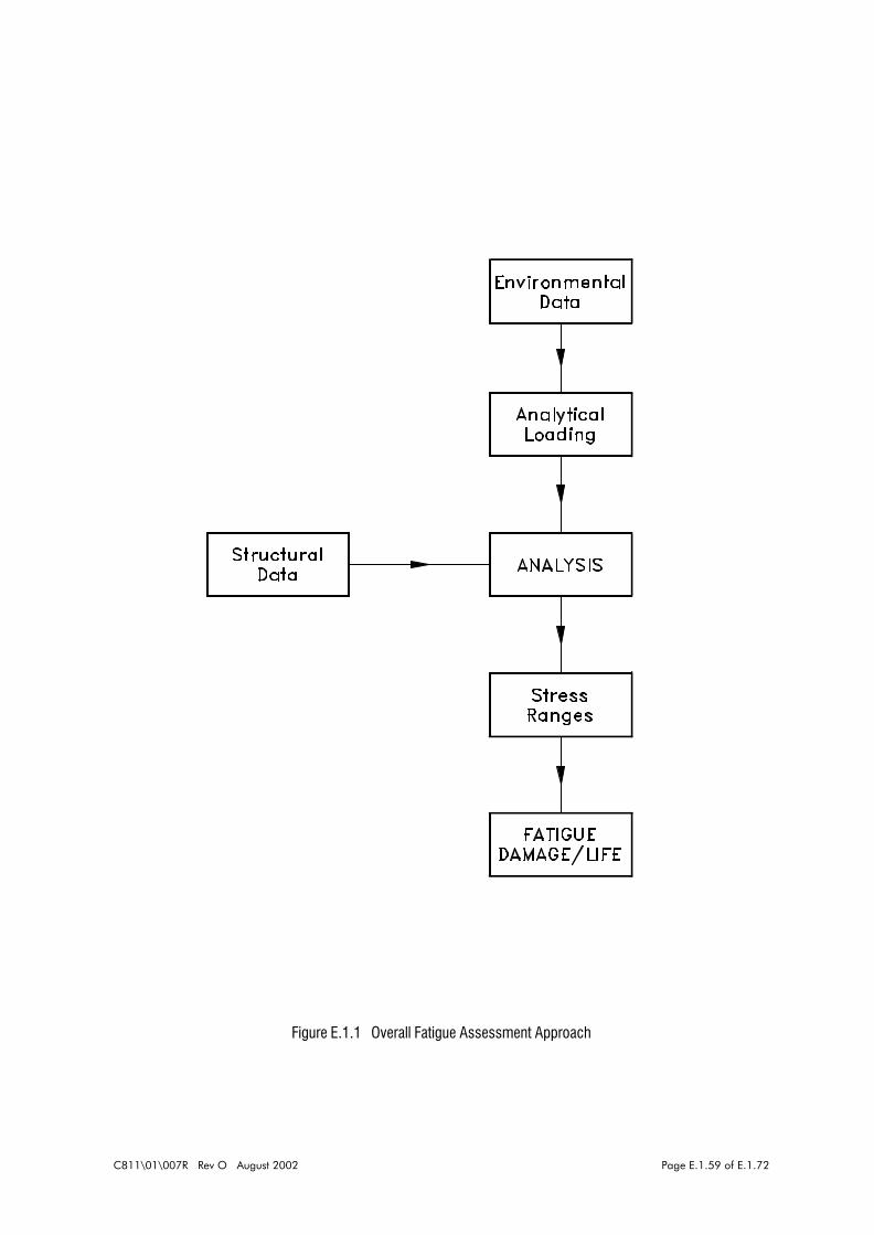
C811\01\007R Rev O August 2002 Page E.1.59 of E.1.72
Figure E.1.1 Overall Fatigue Assessment Approach
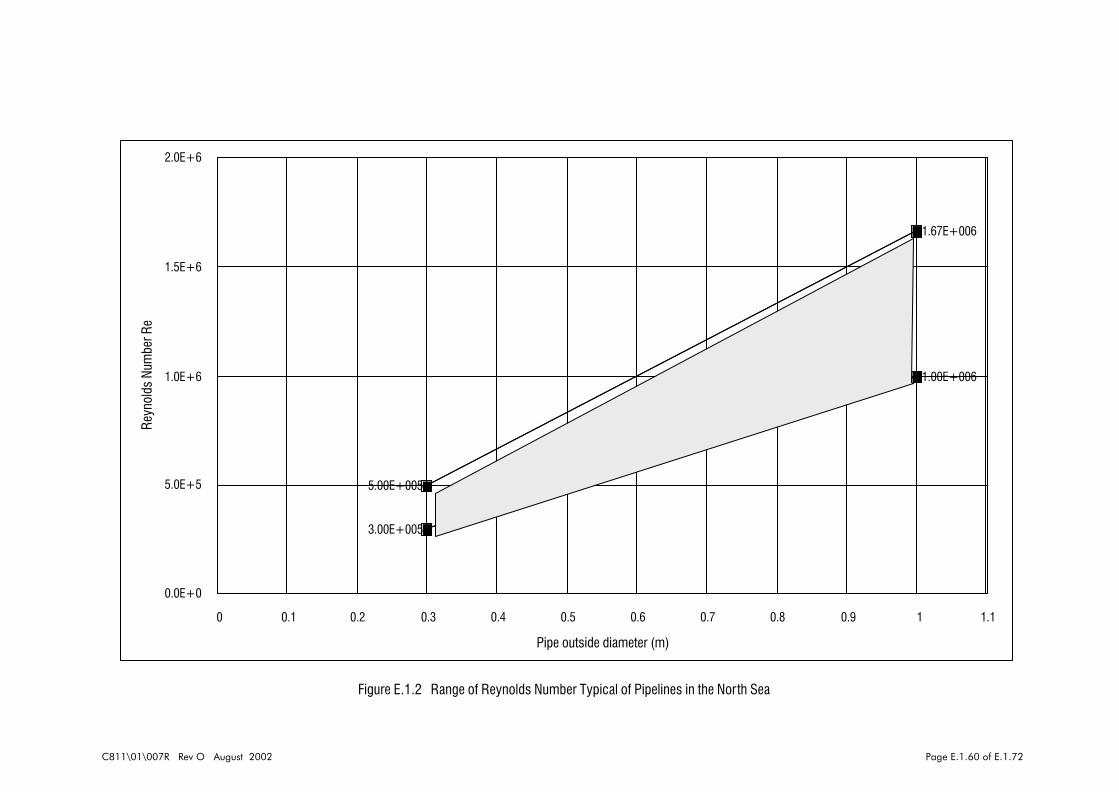
C811\01\007R Rev O August 2002 Page E.1.60 of E.1.72
3.00E+005
5.00E+005
1.00E+006
1.67E+006
0 0.1 0.2 0.3 0.4 0.5 0.6 0.7 0.8 0.9 1 1.1
Pipe outside diameter (m)
0.0E+0
5.0E+5
1.0E+6
1.5E+6
2.0E+6Re
ynol
ds N
umbe
r Re
Figure E.1.2 Range of Reynolds Number Typical of Pipelines in the North Sea

C811\01\007R Rev O August 2002 Page E.1.61 of E.1.72
Figure E.1.3 Strouhal Number as a Function of Reynolds Number for Fixed Rigid Smooth Cylinders in Uniform Flow (Sheppard and Omar, 1992)
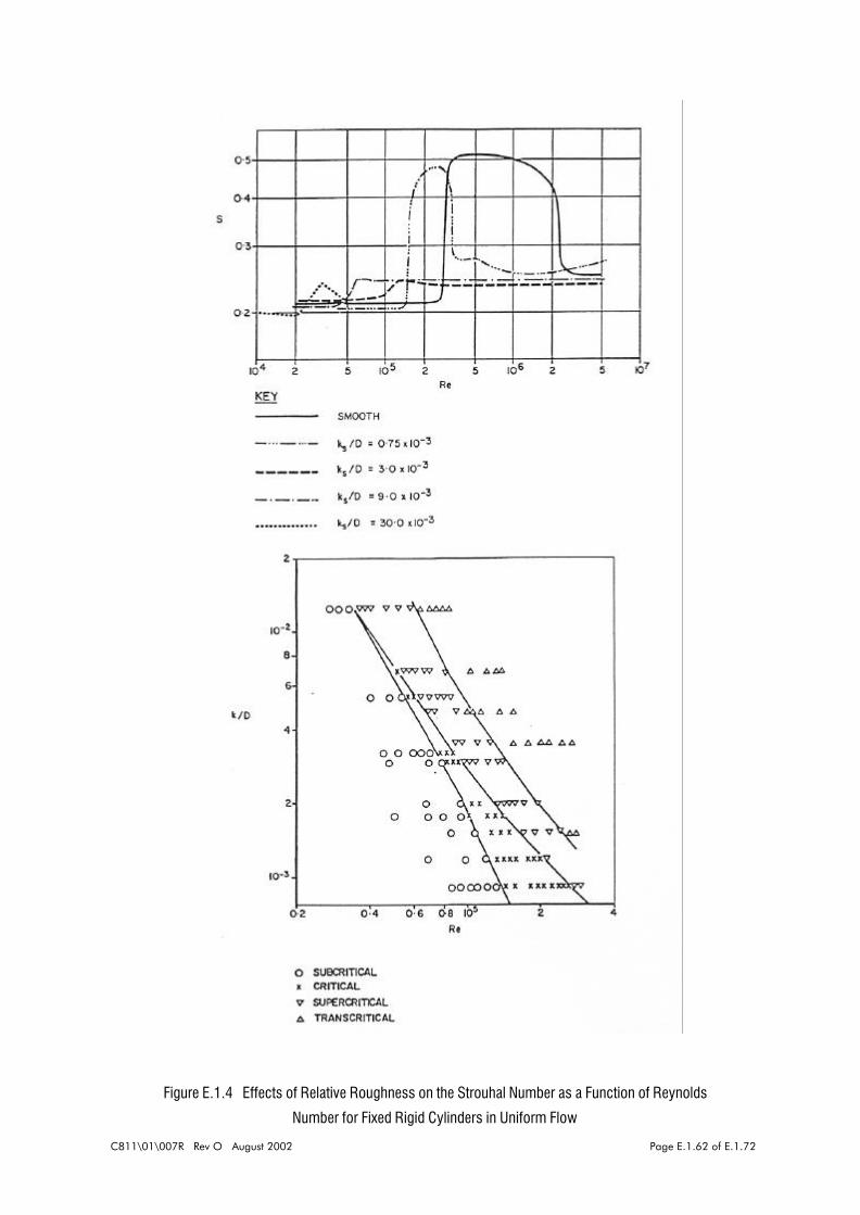
C811\01\007R Rev O August 2002 Page E.1.62 of E.1.72
Figure E.1.4 Effects of Relative Roughness on the Strouhal Number as a Function of Reynolds
Number for Fixed Rigid Cylinders in Uniform Flow

C811\01\007R Rev O August 2002 Page E.1.63 of E.1.72
Figure E.1.5 Idealised Response of a Moveable Cylinder in Uniform Flow

C811\01\007R Rev O August 2002 Page E.1.64 of E.1.72
Figure E.1.6 Flow Chart for Vortex Shedding Checks According to DNV (1981)

C811\01\007R Rev O August 2002 Page E.1.65 of E.1.72
Figure E.1.7 Underlying Graphs for In-Line and Cross-Flow Excitation of Pipelines taken from DNV
(1981)

C811\01\007R Rev O August 2002 Page E.1.66 of E.1.72
Figure E.1.8 Flow Chart for Vortex Shedding Checks According to Barltrop and Adams (1991)

C811\01\007R Rev O August 2002 Page E.1.67 of E.1.72
Figure E.1.9 In-Line Vortex Shedding Graphs from Barltrop and Adams (1991):
Upper: Criteria, Lower: Amplitude of Response

C811\01\007R Rev O August 2002 Page E.1.68 of E.1.72
Figure E.1.10 Cross-Flow Vortex Shedding Graphs from Barltrop and Adams (1991).
Upper: Criteria, Lower: Amplitude of Response
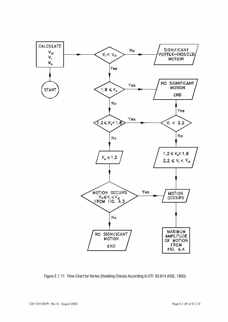
C811\01\007R Rev O August 2002 Page E.1.69 of E.1.72
Figure E.1.11 Flow Chart for Vortex Shedding Checks According to OTI 93 614 (HSE, 1993)
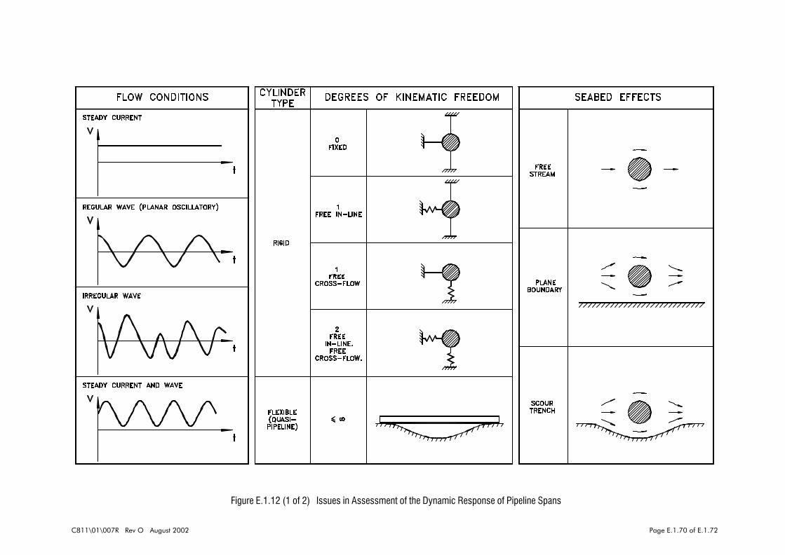
C811\01\007R Rev O August 2002 Page E.1.70 of E.1.72
Figure E.1.12 (1 of 2) Issues in Assessment of the Dynamic Response of Pipeline Spans

C811\01\007R Rev O August 2002 Page E.1.71 of E.1.72
Figure E.1.12 (2 of 2) Issues in Assessment of the Dynamic Response of Pipeline Spans
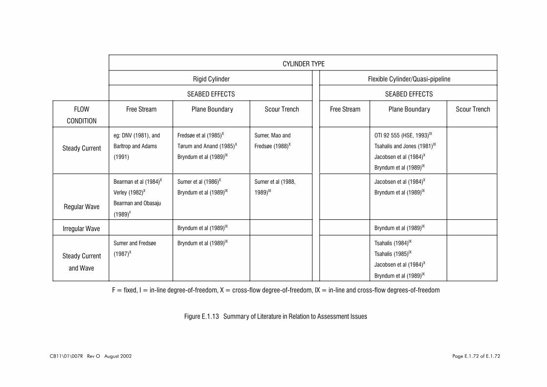
C811\01\007R Rev O August 2002 Page E.1.72 of E.1.72
CYLINDER TYPE
Rigid Cylinder Flexible Cylinder/Quasi-pipeline
SEABED EFFECTS SEABED EFFECTS
FLOW
CONDITION
Free Stream Plane Boundary Scour Trench Free Stream Plane Boundary Scour Trench
Steady Current
eg: DNV (1981), and
Barltrop and Adams
(1991)
Fredsøe et al (1985)X
Tørum and Anand (1985)X
Bryndum et al (1989)IX
Sumer, Mao and
Fredsøe (1988)X
OTI 92 555 (HSE, 1993)IX
Tsahalis and Jones (1981)IX
Jacobsen et al (1984)X
Bryndum et al (1989)IX
Regular Wave
Bearman et al (1984)X
Verley (1982)X
Bearman and Obasaju
(1989)F
Sumer et al (1986)X
Bryndum et al (1989)IX
Sumer et al (1988,
1989)IX
Jacobsen et al (1984)X
Bryndum et al (1989)IX
Irregular Wave Bryndum et al (1989)IX Bryndum et al (1989)IX
Steady Current
and Wave
Sumer and Fredsøe
(1987)X
Bryndum et al (1989)IX Tsahalis (1984)IX
Tsahalis (1985)IX
Jacobsen et al (1984)X
Bryndum et al (1989)IX
F = fixed, I = in-line degree-of-freedom, X = cross-flow degree-of-freedom, IX = in-line and cross-flow degrees-of-freedom
Figure E.1.13 Summary of Literature in Relation to Assessment Issues

C811\01\007R Rev O August 2002 Page E.2.1 of E.2.14
E.2 INITIAL PROPOSAL FOR DYNAMIC METHODOLOGY
E.2.1 PREAMBLE
The purpose of this section of the report is to set out an initial proposal for a dynamic
assessment strategy of pipeline spans, based partly on the review of information contained
within the preceding sections. The scope of the methodology has been widened to cover not
only fatigue but dynamic overstress assessment.
Subsection E.2.2 sets out the generic overall dynamic assessment strategy; this embodies,
within a tiered approach, the interaction between data, load combinations, criteria, analytical
methods and span acceptance. The dynamic overstress and fatigue aspects run in parallel
through the strategy. Attention is paid primarily in this report to the fatigue aspects.
The various components that make up the strategy are dealt with both generically, and in terms
of specifically recommended technologies, in Subsections E.2.3 to E.2.5. Some important
observations regarding the relationship between the proposed and existing methodologies are
made in Subsection E.2.6. Closing remarks are given in Subsection E.2.7. Some areas are dealt
with in reasonable detail, and some in overview terms because the precise make-up will be a
matter of very detailed development, which is outwith the scope of the present work.
E.2.2 OVERALL DYNAMIC ASSESSMENT STRATEGY
E.2.2.1 Overall StrategyThe overall dynamic assessment strategy is summarised in Figure E.2.1, by means of a flow
chart. It adopts a three-tiered philosophy, consistent with the static strength assessment
strategy recommended by BOMEL. As can be seen, the dynamic overstress and fatigue
aspects form two parallel strands within the strategy which dovetail with the static strength
assessment strategy at the points indicated.
The strategy is, in effect, a screening process involving three tiers of assessment which, in
order of application, involve successively less conservatism and more sophisticated analytical
and modelling techniques. In this way pipeline spans that pass conservative tests, that are
designed to be easily and rapidly applied, to bulk-processing of large numbers of spans, are
screened out at an early stage, leaving fewer spans to be analysed using the more complex
techniques of the higher tiers. Thus the basic structure of each tier is similar insofar as it
involves the interaction between data, loading, criteria and an analytical method before a

C811\01\007R Rev O August 2002 Page E.2.2 of E.2.14
decision is made whether to accept a span. A span must be deemed acceptable with respect
to both dynamic overstress and fatigue computations before it is passed to the static strength
assessment strategy. If it is not acceptable in dynamic terms it is passed to the next higher
tier for processing. If a span is determined to be not acceptable at the Tier 3 level, then it must
be rectified.
Differences do exist between the tiers, and these are discussed in more detail in the subsection
referred to in the preamble. In the meantime it is worth noting a few general points regarding
the tiers.
The particular structure of Tiers 1 and 2 is similar. Data form input to the loading, the criteria
and the analytical method. The load combinations are input into the criteria and analysis
elements, and the criteria input into the analytical method. The output from the analytical
method is an allowable span length, which is compared with the observed span length (as
measured in the field survey) to determine the acceptability of the latter.
Three key differences exist between Tier 3, and Tiers 1 and 2. The first is that the observed
span length has been removed from the decision regarding span acceptability, and instead
forms part of the input to the Tier 3 analytical methods. Secondly, instead of the criteria forming
input to the analytical method, they form part of the decision-making process as to whether the
span is acceptable. Thirdly, the output from the Tier 3 analytical methods relate directly to the
criteria employed. Thus observed span lengths are analysed with the results judged against
criteria to determine acceptability.
The key features of this strategy are the fact that it is generic and modular. At this level it is
not tied to particular technologies; advances in terms of criteria, analytical developments, and
improvements in knowledge concerning data and loading can be readily incorporated.
E.2.2.2 Deterministic, Statistical and Reliability-Based StrategiesThe overall dynamic assessment strategy proposed offers sufficient scope and flexibility so as
to allow implementation within a conventional deterministic framework, or a reliability-based
context. In simple terms this is usually regarded as the difference between entering single
values and distributions into governing mathematical models. Notwithstanding this, sight must
not be lost of the fact that all methodologies are statistically based: deterministic values are
generally derived from percentiles of the parameter statistical distributions. These would stem
from a finite, sample population and would be subject to some variation that would generate the
reliability aspects of the problem (see Figure E.2.2).
C811\01\007R Rev O August 2002 Page E.2.3 of E.2.14
Fatigue is a somewhat different problem insofar as it is necessary to consider the damage
resulting from the full range of the distribution of the initiating parameters. The statistics need
to be considered in more depth in what corresponds to a deterministic approach; reliability only
enters the picture if the variability of the statistics, considered as a whole, is also taken into
account.
E.2.3 DATA, LOADING CASES AND LOAD COMBINATIONS
E.2.3.1 DataWith reference to Figure E.2.3 data are divided into three classes: pipeline, environmental and
operational. A more detailed breakdown of the parameters within each class is given in Table
E.2.1. The pipeline data include geometrical and material properties, both mechanical and those
connected with weight. The operational data encompass installation (residual lay tension) and
input related to the pipe contents: its density and pressure. The environmental data include the
parameters that relate principally to the fluid loading on the pipeline (for example, water depth
and various fluid par ticle motion statistics). It might also contain parameters defining the
mechanical interaction between the pipe and the seabed (for example, the soil modulus at the
span shoulders).
The list is not definitive; it depends on which approaches are taken in the analytical methods
within particular tiers. In such circumstances it may be necessary, for example, to add
longitudinal and transverse friction coefficients between the pipe and the seabed soil to the
parameters listed.
E.2.3.2 Loading ClassesThese are also covered in Figure E.2.3. Detailed loadings are those which are either taken
directly from the relevant class of input data, for example: internal pressure, which as shown
comes from the operational data, or are derived using base-level calculations using input from
one or more of the data classes. An example of the latter is external (hydrostatic) pressure,
which is calculated from water depth and local seawater density as contained in the
environmental data class. In terms of detailed thermo-mechanical loads there are seven types
that require considerations:
! submerged weight per unit length
! external temperature
! external pressure
! current and wave-induced uniformly distributed load
! contents weight uniformly distributed load

C811\01\007R Rev O August 2002 Page E.2.4 of E.2.14
! internal temperature
! internal pressure
The data sources for each of these individual loads are indicated by connecting arrows to the
various data classes.
Loading classes incorporating groups of the detailed loadings are also suggested in Figure E.2.3.
Four classes are given, namely:
! self-weight: dead
! environmental: dead
! environmental: live
! operating
The classes are largely self-explanator y and have been designed to differentiate between
loadings that are by and large invariant, or subject to only minor variations (dead), and those
that are more likely to vary with time (live).
The operating class is also live, and it is suggested that more than one type of operating
condition may be need to be addressed. The list given covers normal and maximum allowable
operating conditions, shut down and hydrotest. Between these, differences will exist in internal
temperatures and pressures, and in some cases contents density and hence contents weight
UDL. In some operating conditions some detailed loadings will be absent completely.
E.23.3.3 Load CombinationsClassifying loadings in the way described above allows load combinations to be considered, as
indicated in the figure. Generically speaking, a load combination is made up from a number of
loading classes, and will always comprise both dead loading classes, an operating class, and
the environmental: live loading class. Without the latter there would, of course, be no dynamic
effects to be considered.
E.2.4 ANALYTICAL METHODS
E.2.4.1 Tier 1This being the lowest tier in the overall assessment strategy, it is essential that the analytical
methods employed are:
! conservative

C811\01\007R Rev O August 2002 Page E.2.5 of E.2.14
! relatively (compared to the high tiers) uncomplicated
! easily and rapidly applied.
These requirements are necessary to allow the bulk-processing of large numbers of spans and
the screening out as acceptable of a large majority at an early stage.
For these reasons it is recommended that for the Tier 1 fatigue method (see Figure E.2.1) a
reduced velocity technique is used. In broad terms the approach taken should be similar to that
already employed, whereby a comparison is made between an allowable reduced velocity,
obtained from the span properties and an experimental database, and imposed reduced
velocities stemming from the water particle kinematics. Owing to the inherent uncer tainties in
the whole process the comparison should be statistically based involving the probability of
exceedance of the allowable reduced velocity by the imposed conditions. The reliability aspects
can be introduced by assigning the appropriate variability to the allowable reduced velocity.
E.2.4.2 Tier 2At this tier level the technology to be used should be more complex and less conservative than
that recommended for Tier 1, but should still be readily applicable and involve a dedicated
spreadsheet or high-level computer language programmes. Owing to the statistical nature of
the fatigue process it is recommended that analysis methods should be based around
frequency-domain, rather than time-domain analyses, as these are particularly suited to the
purpose.
Loading should be derived using the model suggested by Pantazopoulos et al (1993), and the
structural model should be based upon theirs but with developments necessary to convert it to
function in the frequency-domain. Careful calibration studies of the overall analytical method
should be made against experimental data with a view to possible simplification to equivalent
single and two degree-of-freedom systems.
E.2.4.3 Tier 3The highest level of analytical sophistication should be applied at this tier in anticipation that the
fewest number of spans will require assessment. On this basis it is recommended that finite
element methods are applied at this stage. ABAQUS (see Subsection E.1.3.3.2) should be
used, and advantage taken of the use of an equilibrium base state of the pipeline arrived at by
means of a nonlinear static analysis. This allows advantage to be taken of higher-order effects,
such as membrane stretching, on the stiffness properties of the pipeline.
Random response analysis should be used, taking as input power spectral density functions
derived from loading defined using the EXXON loading model (Pantazopoulos et al, 1993). The

C811\01\007R Rev O August 2002 Page E.2.6 of E.2.14
principal output from such analyses would be stress-range power spectral densities that would
require post-processing analysis (that is not performed by ABAQUS) to compute fatigue
damage. Modules would need to be developed to undertake these calculations, as well as
modules to pre-process the loading into a form suitable for ABAQUS input.
E.2.5 DETAILED LOADING
E.2.5.1 Data
E.2.5.1.1 Current data
Current data are usually available in the form of scatter diagrams containing current velocity
(measured at some height above the seabed), direction and number of occurrences at each
combination of direction and velocity, as measured at a particular sampling rate over a fixed
period of time. The word diagram is something of a misnomer because the data may be in
tabular form with, for example, the columns corresponding with cardinal compass directions and
the rows with bin ranges of current velocity.
In certain circumstances a degree of processing may have been applied to the data. For
example, individual directional data may have been taken and Weibull distributions fitted. The
two Weibull parameters may then be tabulated against direction.
E.2.5.1.2 Wave data
The random nature of the water sur face means that it can only be quantified statistically (see
Subsection E.2.2.2). The statistics do not change very much over a period of about 3 hours and
a particular seastate may be described by the:
! significant wave height (Hs), and
! the mean zero crossing period (T z).
The significant wave height is the average height of waves that observers will typically repor t
(Barltrop and Adams, 1991). However, it is biased towards the higher waves and is found to
correspond to the average height of the highest one-third of the waves in the seastate.
The mean zero crossing period is obtained from the mean time between up-crossings of the
mean water level. It is dependent on the frequency at which the water surface elevation is
sampled. Various useful relationship regarding the make-up of the wave heights within a
seastate can be derived under the assumption of a Rayleigh distribution.
The significant wave height and mean zero crossing period are typically measured every one
C811\01\007R Rev O August 2002 Page E.2.7 of E.2.14
or three hours. Results are presented in an array, as a seastate scatter diagram; these relate
Hs and Tz to frequency of occurrence at each combination of these two parameters. This may
correspond to a total fixed period of time over which measurements were taken (1 year, 3 years,
etc), and directional variation may also be introduced.
The key points to appreciate with regard to fatigue/dynamic response of pipelines are, therefore:
! over an extended period of time an appreciable number of distinctive seastates may
occur
! an individual seastate is itself statistically based and may be regarded as built-up
from combinations of wave heights and periods.
E.2.5.2 Data ProcessingThe preceding refers to, in a sense, raw current and wave data. This will require pre-processing
into forms suitable as input in the form of "loads" to the various dynamic analysis methods. The
term load is meant here in its most general sense, because some of the dynamic analysis
methods suggested for use above involve reduced velocity techniques; load in that sense
therefore means water particle velocity. Not only this, but the precise requirements as to pre-
processing depend on the details of the analytical methods employed.
A fur ther, and vitally important, question also arises as to the combination of wave and current
to be taken. So far the statistics of current and wave have been discussed individually; the
question as to how joint statistics are to be determined needs to be addressed.
E.2.5.2.1 Current
The principal first step in dealing with the current scatter data is relating the velocities as
recorded at the measurement depth to the velocities at the top of pipe level. According to OTI
93 614 (HSE, 1993) this may be done using either an empirical power law approximation (the
errors produced by which can be of low significance when compared with the uncertainties
inherent in the velocity data), or a logarithmic velocity profile (which is based on a more realistic
physical reasoning, involving turbulent boundary layer theor y and seabed roughness, but
requires a reasonable estimate of the latter from available seabed data).
In addition to this allowance must be made for the yaw angle of the pipeline span under
consideration. This could be achieved by resolving the current velocities to directions normal
and tangential to the span and only considering those normal components. This would need
to be followed by the derivation of a new scatter diagram that eliminates current directional
aspects. What results, therefore, is a one-dimensional array that gives for particular current

C811\01\007R Rev O August 2002 Page E.2.8 of E.2.14
velocities the number of occurrences per year (and, implicitly, the corresponding probabilities).
E.2.5.2.2 Wave
Current data are very easily translated to water particle velocities at the top-of-pipe level. The
situation for wave data is not so straightforward; it would require a number of intervening steps
and calculation loops to perform the required translation from seastate to water particle
velocities and periods at the top-of-pipe level.
As mentioned above the description of a par ticular seastate is itself a statistical representation
of a distribution of component sinusoidal wavelets. The first step in the pre-processing of a
particular seastate is to decompose it to its component wavelets and generate an individual
wave height-period joint probability diagram. This can be achieved using the Longuet-Higgins
formula (see Barltrop and Adams, 1991), which can be applied to calculate the probabilities and,
from the wave periods, the number of waves per year for each seastate occurring in a year.
From this the total number of waves of various heights and periods can be determined by
summing each set of seastate results weighted by each seastate's probabil i ty. The final result
of this step is a single array, each element of which gives the total number of wavelets having
particular combinations of wave height and period occurring during one year.
The second step would be, for each wave height and period in the array, to compute the
corresponding peak water particle velocity at the top of the pipe. Strictly speaking, for each pair
of wave height and period, reference to the water depth should be made and the appropriate
wave theory selected for the computation of the peak horizontal par ticle velocity at the top of
pipe (Barltrop and Adams, 1991). APA (1996) limit the calculation of wave kinematics to Airy
(linear) and Stokes 5th-order wave theories only.
The results of these computations are, therefore, two arrays giving for combinations of wave
height and period in one year:
! the number of waves that occur per year (the probability distribution of combinations
of wave height and period)
! the corresponding peak horizontal velocities.
The combination of these two arrays gives the number of sinusoidal waves per year having a
given peak horizontal velocity at the top of pipe level and period and, implicitly, their
corresponding probability of occurrence as events.
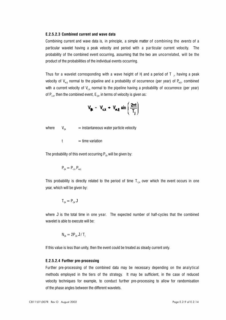
C811\01\007R Rev O August 2002 Page E.2.9 of E.2.14
E.2.5.2.3 Combined current and wave data
Combining current and wave data is, in principle, a simple matter of combining the events of a
particular wavelet having a peak velocity and period with a par ticular current velocity. The
probability of the combined event occurring, assuming that the two are uncorrelated, will be the
product of the probabilities of the individual events occurring.
Thus for a wavelet corresponding with a wave height of Hi and a period of T j, having a peak
velocity of Vw,ij normal to the pipeline and a probability of occurrence (per year) of Pw,ij, combined
with a current velocity of Vc,k normal to the pipeline having a probability of occurrence (per year)
of Pc,k, then the combined event, E ijk, in terms of velocity is given as:
where Vijk = instantaneous water particle velocity
t = time variation
The probability of this event occurring Pijk will be given by:
Pijk = Pc,k Pw,ij
This probability is directly related to the period of time T i j k over which the event occurs in one
year, which will be given by:
Tijk = Pijk J
where J is the total time in one year. The expected number of half-cycles that the combined
wavelet is able to execute will be:
Nijk = 2Pijk J / T j
If this value is less than unity, then the event could be treated as steady current only.
E.2.5.2.4 Further pre-processing
Further pre-processing of the combined data may be necessary depending on the analytical
methods employed in the tiers of the strategy. It may be sufficient, in the case of reduced
velocity techniques for example, to conduct further pre-processing to allow for randomisation
of the phase angles between the different wavelets.

C811\01\007R Rev O August 2002 Page E.2.10 of E.2.14
In the case of structurally-based analytical methods it may be necessary to transform the
velocities into forces, by means for example of the expressions suggested by Pantazopoulos
et al (1993). These in turn may need to be converted to spectra or power density spectra in
order to be in a form suitable for the analytical method concerned.

C811\01\007R Rev O August 2002 Page E.2.11 of E.2.14
Pipeline data
Pipe outside diameter D
Pipe nominal wall thickness t
Corrosion coat thickness te
Weight coat thickness tc
Steel density Ds
Corrosion coat density De
Weight coat density Dc
Steel elastic modulus E
Steel Poisson's ratio <
SMYS steel Fy
Steel thermal expansion coefficient "
Axial restraint factor 8
Operational data
Residual lay tension N
Internal pressure pi
Contents density Di
Contents temperature 2i
Environmental data
Minimum water depth at LAT h
Local sea water density Dw
Local sea water temperature 2a
Hydrodynamic drag coefficient Cd
Hydrodynamic added mass coefficient Cm
Soil modulus at span shoulders Ks
Current statistics
Wave statistics
Table E.1.1 Data Classes for Dynamic Strategy

C811\01\007R Rev O August 2002 Page E.2.12 of E.2.14
TIER 1DYNAMIC METHOD
ACCEPT SPAN ?YES
NO
STATIC STRENGTHASSESSMENT
ALLOWABLESPAN LENGTH
OBSERVED SPANLENGTH
DATA
LOADCOMBINATIONS
CRITERIA
TIER 2DYNAMIC METHOD
ACCEPT SPAN ?YES
NO
LOADCOMBINATIONS
CRITERIA
DATA
ALLOWABLESPAN LENGTH
TIER 3DYNAMIC METHOD
COMPUTED PEAKDYNAMIC STRESS
ACCEPT SPAN ?YES
NO
OBSERVED SPANLENGTH
DATA
CRITERIA:ALLOWABLE
DYNAMICSTRESS,
FATIGUE LIFE
RECTIFY SPAN
LOADCOMBINATIONS
TIER 2FATIGUE METHOD
ALLOWABLESPAN LENGTH
ACCEPT SPAN ?YES
NO
STATIC STRENGTHASSESSMENT
TIER 3FATIGUE METHOD
ACCEPT SPAN ?YES
NO
ACCEPT SPAN ?
NO
RECTIFY SPAN
YESSTATIC STRENGTH
ASSESSMENT
COMPUTEDFATIGUE LIFE
TIER 1FATIGUE METHOD
OBSERVED SPANLENGTH
ALLOWABLESPAN LENGTH
Figure E.2.1 Overall Dynamic Assessment Strategy
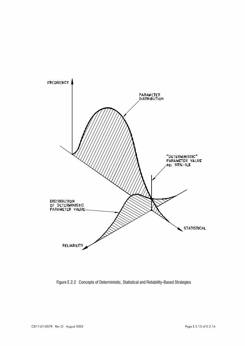
C811\01\007R Rev O August 2002 Page E.2.13 of E.2.14
Figure E.2.2 Concepts of Deterministic, Statistical and Reliability-Based Strategies
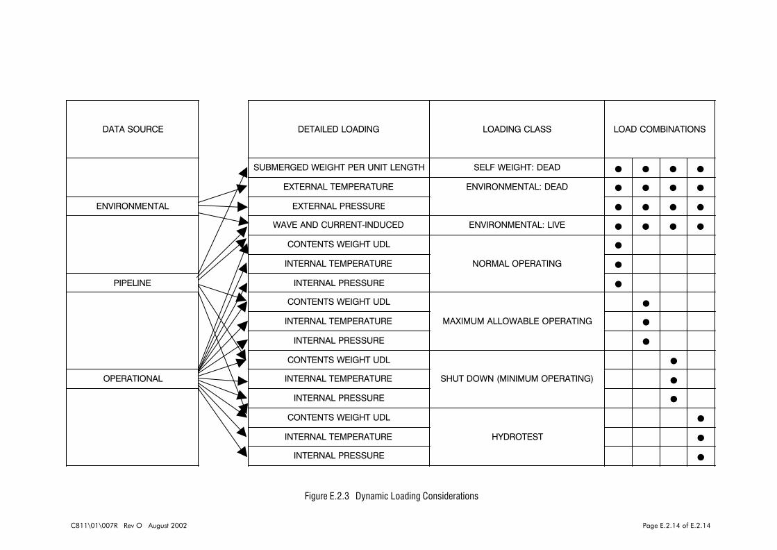
C811\01\007R Rev O August 2002 Page E.2.14 of E.2.14
DATA SOURCE DETAILED LOADING LOADING CLASS LOAD COMBINATIONS
SUBMERGED WEIGHT PER UNIT LENGTH SELF WEIGHT: DEAD · · · ·EXTERNAL TEMPERATURE ENVIRONMENTAL: DEAD · · · ·ENVIRONMENTAL EXTERNAL PRESSURE · · · ·WAVE AND CURRENT-INDUCED ENVIRONMENTAL: LIVE · · · ·CONTENTS WEIGHT UDL ·INTERNAL TEMPERATURE NORMAL OPERATING ·PIPELINE INTERNAL PRESSURE ·CONTENTS WEIGHT UDL ·INTERNAL TEMPERATURE MAXIMUM ALLOWABLE OPERATING ·INTERNAL PRESSURE ·CONTENTS WEIGHT UDL ·OPERATIONAL INTERNAL TEMPERATURE SHUT DOWN (MINIMUM OPERATING) ·INTERNAL PRESSURE ·CONTENTS WEIGHT UDL ·INTERNAL TEMPERATURE HYDROTEST ·INTERNAL PRESSURE ·Figure E.2.3 Dynamic Loading Considerations

C811\01\007R Rev O August 2002 Page E.3.1 of E.3.2
E.3. CONCLUSIONS
E.3.1 Pipeline dynamic response is a complex phenomenon involving fluid dynamics and structural
mechanics in close and complicated interaction. The state of knowledge is far from certain and
reliance has been placed in the past (and for the foreseeable future) on the results of
experimentation.
E.3.2 To date analytical techniques have centred around empirical reduced velocity techniques
founded on the experimental bases referred to above. Whilst this approach is probably
acceptable for threshold vibrations, the data has also been extrapolated for use in more complex
situations to compute fatigue life and damage. The validity of this has not been established.
E.3.3 Fatigue assessment strategies currently employed place complete reliance on a single
analytical technique and in that sense are restrictive because they do not allow for the flexibility
offered by introducing a range of different analytical approaches; in one particular case, use is
made of data from codes of practice that may be judged as outdated.
E.3.4 Much of the data in codes of practice is now out of date. However, there is probably sufficient
literature of quality to cover the main aspects of many practical problems of pipeline span
assessment by reduced velocity techniques.
E.3.5 Codes of practice do not currently allow strain-based types of approaches in fatigue
assessment.
E.3.6 From the limited number of reliable analyses reported in the open literature fatigue life of pipeline
spans is extremely sensitive to span length; life decreases as span length increases
E.3.7 Fatigue is inherently statistical in nature and this, coupled to the complexity and uncertainty of
the physical situation, means that probabilistic approaches recommend themselves.
E.3.8 The rational manipulation of environmental data, seastates and current scatter diagrams, and
their appropriate combination and transformation to seabed kinematics and loads, is central to
the rigour of any analytical tool.
E.3.9 The development of structural mechanics techniques is much less well-advanced. This is
principally because of the difficulties that exist in defining the loading. The EXXON method may
help to remedy this.

C811\01\007R Rev O August 2002 Page E.3.2 of E.3.2
E.3.10 Owing to the statistical nature of fatigue any structural mechanics techniques should be based
around spectral or power spectral density approaches, ie. frequency-domain analysis.
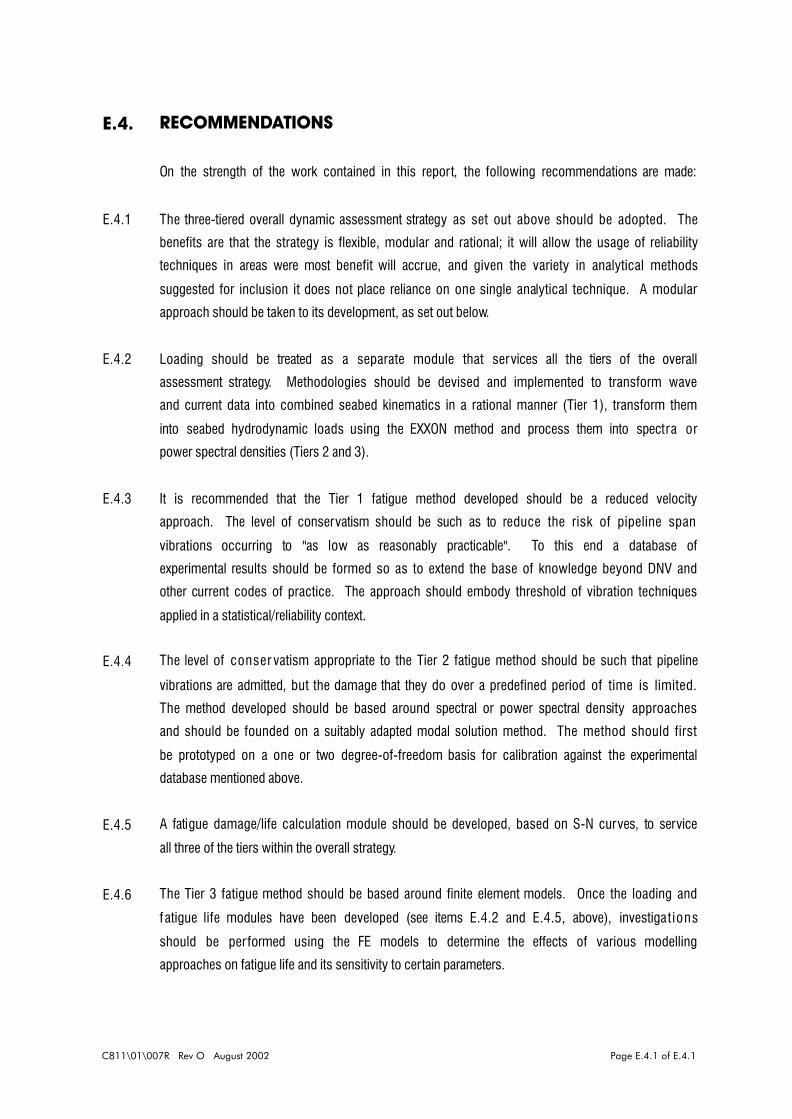
C811\01\007R Rev O August 2002 Page E.4.1 of E.4.1
E.4. RECOMMENDATIONS
On the strength of the work contained in this report, the following recommendations are made:
E.4.1 The three-tiered overall dynamic assessment strategy as set out above should be adopted. The
benefits are that the strategy is flexible, modular and rational; it will allow the usage of reliability
techniques in areas were most benefit will accrue, and given the variety in analytical methods
suggested for inclusion it does not place reliance on one single analytical technique. A modular
approach should be taken to its development, as set out below.
E.4.2 Loading should be treated as a separate module that services all the tiers of the overall
assessment strategy. Methodologies should be devised and implemented to transform wave
and current data into combined seabed kinematics in a rational manner (Tier 1), transform them
into seabed hydrodynamic loads using the EXXON method and process them into spectra or
power spectral densities (Tiers 2 and 3).
E.4.3 It is recommended that the Tier 1 fatigue method developed should be a reduced velocity
approach. The level of conservatism should be such as to reduce the risk of pipeline span
vibrations occurring to "as low as reasonably practicable". To this end a database of
experimental results should be formed so as to extend the base of knowledge beyond DNV and
other current codes of practice. The approach should embody threshold of vibration techniques
applied in a statistical/reliability context.
E.4.4 The level of conser vatism appropriate to the Tier 2 fatigue method should be such that pipeline
vibrations are admitted, but the damage that they do over a predefined period of time is limited.
The method developed should be based around spectral or power spectral density approaches
and should be founded on a suitably adapted modal solution method. The method should first
be prototyped on a one or two degree-of-freedom basis for calibration against the experimental
database mentioned above.
E.4.5 A fatigue damage/life calculation module should be developed, based on S-N curves, to service
all three of the tiers within the overall strategy.
E.4.6 The Tier 3 fatigue method should be based around finite element models. Once the loading and
fatigue life modules have been developed (see items E.4.2 and E.4.5, above), investigat ions
should be performed using the FE models to determine the effects of various modelling
approaches on fatigue life and its sensitivity to certain parameters.
C811\01\007R Rev O August 2002 Page E.5.1 of E.5.4
E.5. REFERENCES
1. ABB Global Engineering (1994). 'Amoco (UK) Exploration Company. Pipeline
engineering support services. Span assessment procedure for Amoco pipelines',
ABBGEL Document No 1723/RPT/0.31 Rev A2, January 1994.
2. American Petroleum Institute (API) (1993). 'Planning, designing and constructing fixed
offshore platforms - Load and Resistance Factor Design', API RP2A LRFD, First
Edition, 1993.
3. American Welding Society (1983). 'Structural welding code', AWS D1.1, 1983.
4. Andrew Palmer and Associates (APAL) (1993). Private communication.
5. Andrew Palmer and Associates (1996). 'Amoco (UK) Exploration Co, CATS gas
trunkline: deterministic span fatigue analysis'. Document No. 606.11.1/TR/300/01/00,
1996.
6. ASME (1986). 'Boiler and pressure vessel: Code Section III', 1986.
7. Barltrop N D P and Adams A J (1991). 'Dynamics of fixed marine structures',
Butterworth Heineman, Oxford, 3rd Edition, 1991.
8. Bearman P W, Graham J M R, and Obasaju E D (1984). 'A model equation for the
transverse forces on cylinders in oscillatory flow', Applied Ocean Research, Volume
6, No 3, 1984.
9. Bearman P W and Obasaju E D (1989). 'Transverse forces on a circular cylinder
oscillating in-line with a steady current', Proceedings Offshore Mechanics and Arctic
Engineering Conference, 1989.
10. British Standards Institution (1993). 'BS 8010 : Part 3 : 1993 Code of practice for
pipelines subsea: design, construction and installation, 1993.
11. Bryndum M B, Bonde C, Smitt L W, Tura F and Montesi M (1989). 'Long free spans
exposed to current and waves: model tests', OTC Paper 6153, Proceedings 21st
Annual Offshore Technology Conference, 1989.

C811\01\007R Rev O August 2002 Page E.5.2 of E.5.4
12. Department of Energy (1989). 'Offshore installations: Guidance on design,
construction and certification', 4th edition, 1989.
13. Det Norske Veritas (DNV) (1981). 'Rules for submarine pipeline systems', 1981.
14. Faltinsen O M (1990). 'Sea loads on ships and offshore structures', Cambridge
University Press, 1990.
15. Fredsøe J, Sumer B M, Andersen J and Hansen E A (1985). 'Transverse vibrations of
cylinder very close to a plane wall', Proceedings 4th Offshore Mechanics and Arctic
Engineering Symposium, 1985.
16. Health and Safety Executive (1993). 'Evaluation of vortex shedding frequency and
dynamic span response, development of guidelines for assessment of submarine
pipeline spans, Background Document One', OTI 93 614, London: HMSO, 1993
17. Health and Safety Executive (1993). 'Vibration of pipeline spans, Development of
guidelines for assessment of submarine pipeline spans, Background document three',
OTI 92 555, London: HMSO, 1993.
18. Institute of Petroleum (1982). 'Pipeline safety code (IP6)', 4th edition, 1982.
19. Jacobsen V, Bryndum M B, Nielsen R and Fines S (1984). 'Vibrations of offshore
pipelines exposed to current and wave action', Proceedings 3rd Offshore Mechanics
and Arctic Engineering Symposium, 1984.
20. Kaye D, Galbraith D, Ingram J and Davies R (1993). 'Pipeline freespan evaluation: a
new methodology', Offshore European Conference, Aberdeen, 1993.
21. Orgill G, Lambrakos K F, Chao J C and Hyden A M (1990). 'Effects of structural
boundary conditions on fatigue life of pipeline spans undergoing vor tex-induced
vibrations', Proceedings 9th Offshore Mechanics and Arctic Engineering Symposium,
1990.
22. Pantazopoulos M S, Cross l ey C W, Orgill G and Lambrakos K F (1993). 'Fourier
methodology for pipeline span vor tex-induced vibration analysis in combined flow',
Proceedings Offshore Mechanics and Arctic Engineering Conference, 1993.

C811\01\007R Rev O August 2002 Page E.5.3 of E.5.4
23. Sheppard D M and Omar A F (1992). 'Vortex-induced loading on offshore str uctures:
a selective review of experimental work', OTC Paper 6817, Proceedings 24th Annual
Offshore Technology Conference, 1992.
24. Snamprogetti Limited (1994). 'Report to Amoco on: Study to investigate free spanning
of Southern North Sea pipelines'.
25. Sumer B M, Fredsøe J and Jacobsen V (1986). 'Transverse vibrations of a pipeline
exposed to waves', Proceedings 5th Offshore Mechanics and Arctic Engineering
Symposium, 1986.
26. Sumer B M and Fredsøe J (1987). 'Transverse vibrations of an elastically mounted
cylinder exposed to an oscillating flow', Proceedings 6th Offshore Mechanics and
Arctic Engineering Symposium, Vol II, 1987.
27. Sumer B M, Mao Y and Fredsøe J (1988). 'Interaction between vibrating pipe and
erodible bed'. Journal of Waterway, Port, Coastal and Ocean Engineering, Proceedings
ASCE, Vol 114, No 1, 1988.
28. Sumer B M and Fredsøe J (1988). Vibrations of pipelines in scour trenches',
Proceedings BOSS, Vol 2, 1988.
29. Sumer B M, Fredsøe J, Gravesen H and Bruschi R (1989). 'Response of marine
pipelines in scour trenches', Journal of Waterway, Port, Coastal and Ocean
Engineering, Proceeding ASCE, Vol 115, No 4, 1989.
30. Tørum A and Anand N M (1985). 'Free span vibrations of submarine pipelines in
steady flows - effect of free-stream turbulence on mean drag coefficients', Journal of
Energy Resources Technology, Transactions ASME, Vol 107, 1985.
31. Tsahalis D T and Jones W T (1981). 'Vortex-induced vibrations of a flexible cylinder
near a plane boundary in steady flow', OTC Paper 3991, Proceedings 24th Annual
Offshore Technology Conference, 1981.
32. Tsahalis D T and Jones W T (1982). 'The effect of sea-bottom proximity on the
fatigue life of suspended spans of offshore pipelines undergoing vortex-induced
vibrations', OTC Paper 4231, Proceedings 25th Annual Offshore Technology
Conference, 1982.
C811\01\007R Rev O August 2002 Page E.5.4 of E.5.4
33. Tsahalis D T (1983). 'The effect of sea bottom proximity of the vortex-induced
vibrations and fatigue life of offshore pipelines', Journal of Energy Resources
Technology, Transactions ASME, Vol 105, 1983.
34. Tsahalis D T (1984). 'Vortex-induced vibrations of a flexible cylinder near a plane
boundary exposed to steady and wave-induced currents', Journal of Energy Resources
Technology, Transactions ASME, Vol 106, 1984.
35. Tsahalis D T (1985). 'Vortex-induced vibrations due to steady and wave-induced
currents of a flexible cylinder near a plane boundary', Proceedings 4th Offshore
Mechanics and Arctic Engineering Symposium, 1985.
36. Verley R L P (1982). 'A simple model of vortex-induced forces in waves and
oscillating currents', Applied Ocean Research, Vol 4, No 2, 1982.

C811\01\007R Rev O August 2002 Page F.0.1 of F.0.3
APPENDIX F
CRITERIA DETERMINING THE STATIC
STRENGTH OF PIPELINE SPANS

C811\01\007R Rev O August 2002 Page F.0.2 of F.0.3
TABLE OF CONTENTS
Page No
F.1 CRITERIA DETERMINING THE STATIC STRENGTH OF PIPELINE SPANS
F.1.1 PREAMBLE
F.1.2 STRESS AND STRAIN CRITERIA SET BY CODES
F.1.2.1 Stress Criteria
F.1.2.2 Strain Criteria
F.1.3 OFFSHORE TECHNOLOGY REPORT OTN 94 186 (1994)
F.1.3.1 Review of Codes and Guidelines
F.1.3.2 Reviews of Technical Information related to Pipeline Ovalisation
and Strength
F.1.3.3 Effects of High Strain Bending on Material Properties
F.1.3.4 Initial Proposal for Strain-Based Assessment Framework
F.1.4 JIP ON THE ESTABLISHMENT OF STRAIN-BASED CRITERIA AND
ANALYSIS FOR THE ASSESSMENT OF SUBSEA PIPELINES
F.1.4.1 Objective of the Project and Scope of Work
F.1.4.2 Review of Principal Sections of Final Report
F.1.5 COMPARISON OF STRAIN LIMITS
F.1.5.1 Pipeline Considered
F.1.5.2 Preliminary Results and Basis of Comparison
F.1.5.3 Results from Comparison
F.1.6 CLOSING REMARKS
F.1.7 REFERENCES
F.1
F.1
F.1
F.2
F.2
F.4
F.4
F.7
F.10
F.11
F.12
F.12
F.13
F.18
F.18
F.18
F.22
F.23
F.23

C811\01\007R Rev O August 2002 Page F.0.3 of F.0.3
LIST OF TABLES
Table F.1.1 Coverage detail of strain-based assessment in codes reviewed in OTN 94 186
(1994)
Table F.1.2 Coverage detail of strain-based assessment in AME (1996) [As Table 3.1, but
updated to include RP 1111]
Table F.1.3 Pipeline data
Table F.1.4 Pipeline results (full axial fixity assumed)
Table F.1.5 Pipeline Results: strain limits from AME formulae (AME, 1996) and BS8010/DNV
formulae in terms of bending strain and equivalent plastic strain increment

C811\01\007R Rev O August 2002 Page F.1 of F.29
F.1. CRITERIA DETERMINING THE STATIC STRENGTH OF PIPELINE
SPANS
F.1.1 PREAMBLE
The purpose of this appendix is to address the criteria available to determine the limiting span
length of pipelines with respect to static strength. Attention has concentrated on strain limits,
as this approach appears to offer more scope for the safe relaxation of criteria than the more
conventional stress-based methods.
Section F.1.2 presents an overview of two codes that would be the most important in terms of
North Sea practice. These have been taken because they represent the best level of detail
offered by all of the pipeline codes taken together. This fact is confirmed by Section F.1.3,
which gives a summary of a review under taken for the UK Health and Safety Executive on
structural and material implications of bending pipelines to large strains. This involved a review
of design codes/guidelines, as well as relevant technical information. Section F.1.4 reviews the
Final Report of a large Joint Industry Project conducted by a third party contractor of which
Amoco was one of the sponsors. The objective of the project was to establish a capability and
provide information for the analysis and assessment of pipelines based on strain criteria. The
scope of work covered pipe and material testing and finite element work. A comparison
between the strain limits proposed by the JIP document, and those from codes and guidelines,
is made for an example pipeline segment from Amoco's operations in Section F.1.5. Closing
remarks are to be found in Section F.1.6.
F.1.2 STRESS AND STRAIN CRITERIA SET BY CODES
The two codes considered in this respect are typical of those available, they are:
! BS 8010 : Part 3 : 1993
Code of Practice for Pipelines Subsea: design, construction and installation.
! Det Norske Veritas (DNV) : 1981 (Reprint with corrections 1982)
Rules for Submarine Pipeline Systems
Within these document the design conditions that are relevant to the spanning situation are
referred to as:
C811\01\007R Rev O August 2002 Page F.2 of F.29
! Functional and environmental loads
including: self-weight, thermal effects, pressure effects, transient operations effects,
environmental pressure, residual installation loads; current, wave and wind loadings
(BS 8010)
! Pipeline system during operation
[presumably acted upon by the same set of effects and loadings as listed above
for BS 8010] (DNV).
Both codes allow the use of stress and strain criteria applied to their respective design
conditions as summarised below.
F.1.2.1 Stress CriteriaThe same stress criterion is used by both codes; the maximum equivalent stress in the pipeline
(computed from the von Mises expression) should be less than a design or usage factor times
the specified minimum yield stress (SMYS) of the pipe steel. This is expressed mathematically
as:
/[Fx2 + F2
2 - FxF2] # 8Fy
where Fx = longitudinal stress
F2 = hoop stress
8 = design/usage factor = 0.96
Fy = specified minimum yield stress
F.1.2.2 Strain CriteriaBS 8010 allows alternative design for strain for conditions other than construction loads and
hydrostatic testing and states that:
"The limit on equivalent stress recommended above may be replaced by a limit on allowable
strain, provided that the following conditions are met".
It sets out four conditions that must be adhered to, plus a warning in respect of upheaval
buckling, as follows:
a. Under maximum operating temperature and pressure, the plastic component of the
equivalent strain does not exceed 0.1%. The reference state for zero strain is the
as-built condition (af ter pressure testing).

C811\01\007R Rev O August 2002 Page F.3 of F.29
b. Any plastic deformation occurs only when the pipeline is first raised to its
maximum operating pressure and temperature, but not during subsequent cycles of
depressurisation, reduction in temperature to the minimum operating temperature,
or return to the maximum operating pressure and temperatures.
c. The ratio of outside diameter to thickness of the pipe does not exceed 60.
d. Welds have adequate ductility to accept plastic deformation.
Finally, the influence of the plastic deformation on the pipeline's resistance to upheaval buckling
should be checked if this phenomenon is likely to occur.
DNV also allows the use of strain criteria in respect of design for the operation condition and
states that:
"...In cases where possible strain (displacement) does not exceed the permissible strain ...
stresses need not be used as a criterion against excessive yielding...".
The permissible strain is not quantitatively prescribed, but its magnitude must:
a. Take account of the material ductility
b. Take account of previously experienced plastic strain (during installation, for
example)
c. Result in acceptable fracture toughness af ter deformation under this condition
d. Not lead to violation of out-of-roundness limitations.
These requirements apply to conditions of permanent strain (arising from, for example,
permanent curvature) and to pipelines in (almost) continuous contact with the seabed, and to
pipelines not in continuous contact provided that yielding would lead to contact that arrested
strains before they exceed the permissible values.
To summarise: strain limits are set explicitly by BS 8010, but DNV only gives criteria on which
to base limiting strain centred around material requirements, ovalisation and local buckling.

C811\01\007R Rev O August 2002 Page F.4 of F.29
F.1.3 OFFSHORE TECHNOLOGY REPORT OTN 94 186 (1994)
This document constituted a comprehensive review of the design codes/guidance and available
technical literature relevant to the structural and material implications of bending pipelines to
large strains. It covered the following areas:
! Review of codes and guidelines
! Reviews of technical information related to
- Ovalisation in response to bending
- Pipeline strength under individual and/or combined loading actions
! Tests elucidating the effects of high strain bending on material properties
! Initial proposal for strain-based assessment framework.
In addition to these, Appendices covered representation of material stress-strain behaviour,
plasticity equations and methods for ovalisation computation.
The subsections that follow summarise the principal areas listed above.
F.1.3.1 Review of Codes and GuidelinesThe review of codes and guidelines covered the following six documents:
1. Submarine Pipeline Guidance Notes. Issued by the Pipeline Inspectorate, Petroleum
Engineering Division, Department of Energy, October 1984 (DEnGN).
2. Model Code of Safe Practice in the Petroleum Industry: Part 6 Pipeline Safety Code.
Institute of Petroleum, 4th Edition, December 1982. Plus Supplement, August 1986
(IP6).
3. Gas Transmission and Distribution Piping Systems. ASME code for Pressure Piping,
B31 ANSI/ASME B31.8 - 1989. Plus addenda, B31.8a - 1990, B31.8b - 1990 and
B31.8c - 1992 (B31.8).
4. Liquid Petroleum Transpor tation Piping Systems. ASME Code for Pressure Piping,
B31. ANSI/ASME B31.4 - 1979 (B31.4).

C811\01\007R Rev O August 2002 Page F.5 of F.29
5. Rules for Submarine Pipeline Systems. Det Norske Veritas, April 1981, reprint with
corrections 1982 (DNV).
6. Code of Practice for Pipelines. Part 3. Pipelines subsea design, construction and
installation. BSI, BS 8010 : Part 3 : 1993 (BS8010).
A seventh document:
7. Recommended Practice for Design, Construction, Operation and Maintenance of
Offshore Hydrocarbon Pipelines. American Petroleum Institute API RP1111, 1993
(RP1111)
is relevant but was not included in the review.
Each of the codes and guidelines listed above was reviewed under the following headings:
a. Conditions under which strain-based design would be acceptable
b. Allowable strain limits in combination with other loads
c. Buckling
d. Ovalisation
e. Effects of cumulative plastic strain
f. Requirements for straightness following bending/straightening
g. Effects on material properties, including toughness
h. Requirements for welded sections.
i. Recommendations on relevant testing, eg strain ageing, Charpy etc.
j. Guidelines on the implications of low cycles fatigue for cases of repeated cycles
of bending/straightening.
The detailed conclusions in respect of codes/guidelines as they relate to pipeline spanning
(assuming that spanning is relevant to clauses related to pipeline systems during operation)
were as follows:
! Most codes reviewed are similar in that design is divided into two phases: installation
and operation. BS8010, DNV and B31.8 allow strain-based design to be used in both
phases, the other codes make no reference to it. For the most part strain-based
design is allowed in situations of predictable, non-cyclic, strain-limited displacement.
BS8010, in the operation design phase, sets a limit to the pipe D/t ratio of 60.

C811\01\007R Rev O August 2002 Page F.6 of F.29
! Allowable strain limits are dictated, non-specifically, by:
- material ductility
- weld properties
- plastic strain history
- fracture toughness
- buckling
- ovalisation limitations.
BS8010 limits the additional equivalent plastic strain in the operation phase to
0.1%. DNV places no limit other than as determined by the above criteria in the
operation phase (see Section F.1.2.2, above).
! Most codes reviewed in the study require that the following modes of buckling are
checked:
- local pipe wall buckling
- propagation buckling
- restrained bar buckling.
Only BS8010 and DNV provide a range of formulations for these calculations, but of
these only some of the BS8010 formulae are written in terms of strains. IP6
provides a pressure-only formula for local buckling.
! Codes reviewed require that ovalisation be limited. BS8010 provides a formula for
calculations, but sets no prescribed limits, except that a minimum of 2.5% is to be
used in buckling calculations. DNV prescribes a permissible ovalisation (BS8010
definition) of 1%. IP6 insists on a minimum ovalisation in buckling calculations of 1%.
! Guidelines on cumulative plastic strain are given only in the case of BS8010.
! There are no requirements for straightness following bending/straightening except as
may be embodied in residual strain limitations.
! In general there is no specific guidance in respect of the effects on material properties
of large straining. Guidance is limited to the specification of testing to ensure that
material properties are still acceptable.
! The requirements for welded sections are, in general, restricted to the provision of
adequate ductility and fracture toughness, and to the limiting of hardness. For
straining in excess of 5% of C-Mn and C-Mn fine grain treated steels DNV requires

C811\01\007R Rev O August 2002 Page F.7 of F.29
that welds are heat treated and are to have a hardness not exceeding 260 HV5.
! Most codes reviewed allow for the provision of additional testing if service conditions
dictate that it is required, and this may encompass hardness, Charpy V-notch impact
and crack tip opening displacement (CTOD) testing. DNV recommends strain ageing
testing for materials that have been strained in excess of 3%.
! No particular recommendations are made in respect of the implications of low cycle
fatigue in cases of repeated cycles of bending and straightening. Most codes state
that such effects should be incorporated within the normal fatigue check calculations.
In general terms it was concluded that:
! Many of the currently available Codes incorporate the possibility of the use of strain-
based criteria in the assessment of the strength and deformation of pipelines.
! There is no consistency from one Code to another with regard to the strain levels
which may be permitted in assessment.
! There is not a comprehensive set of formulations which could be used together with
strain-based criteria for the assessment of pipelines.
Table F.1.1, taken from OTN 94 186, summarises the findings of the document review.
Columns of the table correspond to the documents reviewed, whilst the rows correspond to
the headings listed (a) to (j), above. Each row/column intersection is given a subjective
grading according to the detail of coverage given to the subject by the document.
It should be borne in mind that the category given to subject areas must be viewed within
the context of its detailed level of coverage as it relates to strain-based assessment
techniques. For example, the DNV document gives a well-detailed formulation for
addressing the problem of local buckling [part of subject © in the table] under load
combinations, but it is stress-based and would be extremely difficult (if not impossible) to
alter its make-up to be expressed in terms of strains. Coverage of the same subject by
BS8010 has been deemed to be 'better' by virtue of the fact the formulations given are
partially strain-based.
F.1.3.2 Reviews of Technical Information related to Pipeline Ovalisation and
StrengthThe purpose of this section of the OTN document was to survey and review the technical

C811\01\007R Rev O August 2002 Page F.8 of F.29
information in the public domain (that was current at the time) which would allow engineers to
evaluate the strength and safety of pipelines at large strains. Attention was concentrated on
information related to ovalisation and strength under individually or collectively applied bending,
pressure and axial force.
The principal conclusions from this review were as follows:
! The Brazier type of elastic analysis (with Poisson's ratio taken as 0.3 and 0.5) greatly
overestimates ovalisations and, whilst conservative, may be uneconomic in practice.
! In modelling ovalisation analytically the following features should be included:
- elasto-plastic material constitutive behaviour
- longitudinal and circumferential stress/strain interaction
- plasticity growth
- longitudinal bending and ovalisation interaction
- pressure and axial loading
- initial states of out-of-roundness, strain and stress and longitudinal
curvature
- cycles of bending, unloading followed by re-bending or reverse bending.
! Few analytical techniques developed to date are able to model the majority of the
effects listed above. Results from most of the techniques have poor correlation with
experimental data, and currently are not in a form that would permit their application
to pipeline assessment.
! Of the techniques examined in this study a particular analytical approach was shown
to provide promising potential in respect of ovalisation calculation. It gives very good
predictions when validated with the limited amount of good experimental data
available. However, it would require fairly extensive development in order to
incorporate the str uctural aspects listed above for a pipeline subjected to pressure
and axial loading including initial states and cycles of bending.
! The experimental data currently available are focused on buckling and, to a less
extent, on ovalisation. Little data is available in respect of extensive strain
measurement in order to assess strain interaction and plasticity growth.
! Few tests have been performed to relate material properties (yield strength, ultimate
strength, toughness and so forth) post-straining to those extant in the as-received
condition. Results from available tests indicated that straining had the effects of

C811\01\007R Rev O August 2002 Page F.9 of F.29
increasing the yield and ultimate strength, reducing the toughness, and increasing the
brittle/ductile transition temperature but these effects are related to older material
properties and may not be relevant to current pipeline steels.
! In respect of pure bending a flexure collapse formula must account for the differing
responses of low and high diameter-to-thickness ratio pipes. It will be required to
highlight the different failure modes for the full practical range of D/t ratios.
! There is a body of evidence that for the low D/t ratio pipes, collapse under pure flexure
may occur at a bending strain very close to that of the collapse axial strain under pure
axial compression. Verification of this is not currently possible owing to the lack of
adequate experimental data for the flexural collapse of pipelines in the range
10<D/t<40.
! Assessment of collapse under pure external pressure needs to consider the fact that
low diameter-to-thickness ratio pipes, in the absence of initial imperfections, collapse
in a plastic bifurcation mode rather than a hoop yield mode. Design formulae based
on this latter concept may have a built-in lack of conservatism.
! Pressure collapse is imperfection sensitive. In the light of the fact that installation
techniques may induce appreciable residual ovalisations, a rational basis for the
computation of collapse pressure for ovalised pipes should account for this.
! To become relevant to a strain-based assessment regime, formulae for predicting
collapse under individual loading (for example, axial compression and pressure) must
reflect material response adequately in terms of plastic buckling (rather than through
attainment of yield stress) through the use of tangent/secant moduli approaches.
! Simplified theories (ie. those not involving FE analysis) for computing strains when
pipes are stressed inelastically and in which geometric non-linearities (buckling) can
be ignored, can be evolved from the mathematical theory of plasticity and be designed
to be perfectly general in terms of loads applied, boundary conditions and so forth.
! In all cases involving the plastic deformation of pipes under load combinations it is
important to emphasise that the order, and manner, of load application affects the
results in terms of plasticity growth and the magnitude of forces necessary for
collapse.
C811\01\007R Rev O August 2002 Page F.10 of F.29
! The effect of axial tension, when in a situation of combined tension and bending, is
beneficial. It increases the magnitude of bending strain at which buckling occurs in
a power-law manner. Formulae available in codes of practice to cover this form of
inter-action either ignore this, or are not clear on the fundamentally different effects
of axial tension and compression.
! Virtually no information was then available to formulate the basis of collapse
envelopes for pipes under the combined action of flexure and axial compression.
! No simple formulations were then available to cover the situation of internal pressure
combined with flexure. Evidence does exist, in the form of a limited quantity of
experimentation and finite element studies (insufficient in total to provide a basis for
the development of rational rules), that the presence of internal pressure has an
ameliorating effect on the consequences of bending: ovalisation may be greatly
reduced and bending buckling strains increased (possibly to the extent that, to all
practical purposes, buckling is eradicated).
! External pressure has a profound effect on collapse under flexure, and this is due to
the interaction of two destabilising force actions. Experimentation and finite element
studies tend to suggest that collapse pressures are reduced by bending strains. This
produces a collapse envelope that is convex-in, thus rendering linear collapse
envelopes (as used in some codes of practice to quantify this interaction) inherently
un-conservative.
! Successful analytical techniques have been evolved in the literature for the prediction
of collapse envelopes, particularly so for the combined external pressure and flexure
combination of loading. These techniques appear to correlate well with experimental
results. However, development of these techniques into design office tools would
require considerable effort.
F.1.3.3 Effects of High Strain Bending on Material PropertiesThe OTN report presented the results of various tests to evaluate the effects on material
properties of bending pipe to high strain levels and straightening. The results relate to only two
grades of steel, viz X42 and X52. The tests included:
! Bending of pipe during which the applied moments and strains were measured
! Tensile tests on specimens of material cut from pipes af ter bending and straightening
and also from pipes in the as-delivered state
C811\01\007R Rev O August 2002 Page F.11 of F.29
! Charpy impact tests on coupons machined from sections of pipes both prior to
bending and af ter bending and straightening.
The following conclusions are drawn from a study of the results of the tests:
! The material yield stress is affected by straining to high levels, but not in a manner
such as to reduce the strength of the material
! The ultimate stress of the material is not affected by bending pipes to high levels of
strain
! The ductility of the material is reduced, but not significantly when the pipe is bent and
straightened
! The toughness of the material, as measured by the failure energy in the Charpy
impact test, is not significantly affected by subjecting the material to high levels of
pre-strain of the bending-type used in the tests
! The toughness of the material in the weld affected zone is well in excess of that
required in Codes for the material tests reported in the document.
Generally it should be noted that the tests reported and the conclusions relate to one cycle of
bending and straightening. That is, the results are relevant to the assessment of the affects on
material properties due to installation by reeling or passing through a J-tube or by the pipe
conforming to the seabed contour. There is no information available to guide engineers on the
assessment of the fitness for purpose of pipelines which have been subjected to moderate or
large strains during a number of cycles of loading. Such situations may occur due to
operational start-up and shut-down processes.
This last situation is very relevant to the design and assessment of high-pressure high-
temperature pipelines and it was recommended that tests on materials likely to be used in
pipelines during the next ten years should be tested under realistic conditions of applied strains
to determine the effects on the material properties over a practical number of cycles.
F.1.3.4 Initial Proposal for Strain-Based Assessment FrameworkThe OTN document also presented some preliminary guidance to engineers involved in the
assessment of pipelines who wished to use the state of knowledge, that was current at that
time, of strain-based criteria. The guidance took the form of a number of points, some of which
recommended the use of calculation techniques developed and detailed in the document. These

C811\01\007R Rev O August 2002 Page F.12 of F.29
comprised: simplified elasto-plastic strain analyses in cases where no large geometric changes
under loading occur; various Perry-based formulations for the strength of pipelines under
individually applied bending, external pressure and axial compression; and formulations for the
strength under load combinations. It was recommended that none of the preliminary guidance
should be applied to situations where large strains are imposed during more than two cycles
of bending or application of pressure and temperature loading.
F.1.4 JIP ON THE ESTABLISHMENT OF STRAIN-BASED CRITERIA AND
ANALYSIS FOR THE ASSESSMENT OF SUBSEA PIPELINES
F.1.4.1 Objective of the Project and Scope of Work The objective of the project (AME, 1996) was to establish a capability and provide the
information for, the analysis and assessment of pipelines based on strain criteria. The scope
of work covered the following:
i. Perform tests on a range of pipe geometries and materials and assemble details of
other tests to provide a basis for the validation of numerical and other analysis
used during design and assessment.
ii. Validate using the test results a range of finite element models which can be used
to simulate the behaviour of pipelines.
iii. Establish, using parametric studies undertaken with a standard finite element
program, a comprehensive description of the structural and material behaviour of
pipelines which are strained beyond the elastic limit in a variety of loading
conditions.
iv. Derive simplified relationships between loading and response for pipelines based
on the finite element parametric studies.
v. Establish strain-based criteria which can be used in design and assessment
vi. Provide guidance on the use of strain-based criteria in the design and assessment
of pipelines.
The Final Report for the project (AME, 1996) was very comprehensive and detailed, running to
nine section (Section 1 being the introduction, and Section 9 providing the references) and nine
appendices (Appendix A to Appendix I). The Appendices covered detailed information not central

C811\01\007R Rev O August 2002 Page F.13 of F.29
to the main thr ust of the report, and these are not reviewed here. The other Sections of the
report contained the following:
Section No Scope
2
3
4
5
6
7
8
Review of design codes and guidelines
Review of previous work on pipeline behaviour
Pipeline testing
Finite element modelling
Parametric studies
Reliability-based assessment methodology
Design guidance
F.1.4.2 Review of Principal Sections of Final Report
F.1.4.2.1 Sections 2 and 3
These sections essentially repeat much of the information contained in the Offshore Technology
Report OTN 94 186 (see Subsection F.1.2, above). The principal exception, however, was the
fact that RP1111 was also reviewed under the same basis as the other documents. It added
very little to the background information, as may be seen from Table F.1.2 (taken from Table 2.8
in the Final Report) where its coverage of strain-based approaches has been classified as no
detail to poorly detailed, or poorly detailed to partly detailed.
F.1.4.2.2 Section 4: Pipeline testing
The objective of the tests was to obtain information on the behaviour of pipelines loaded in
bending beyond their elastic limit. Overall, the tests were divided into two types: bending tests
on prototype scale pipeline segments and material tests on tensile coupons extracted from the
pipes.
The bending test programme comprised different pipe geometries (diameter to thickness ratios
in the range 10-35) and different materials (API grades X52 to X70 and a single Duplex test).
A total of 36 tests was undertaken with a view to determining the response to bending, including
local buckling and ovalisation. The tests involved cycles of bending and reverse bending to
various levels of strain. Both high and low strain cyclic bending were considered. The key
parameters from the bending tests were:
a. moment versus curvature (longitudinal strain) curve
b. pipeline collapse behaviour
C811\01\007R Rev O August 2002 Page F.14 of F.29
c. diameter changes/ovalisation
d. hoop strains
Material tests were performed on specimens taken from each section of pipe involved in the
bending tests, with the intention of determining the effect of applied strain on material
properties. Thus, coupons were extracted from regions of a tested pipe that had been subjected
to maximum strain and least strain. The material properties/characteristics evaluated were:
a. stress-strain curve
b. elastic modulus
c. yield strength
d. strain hardening modulus
e. Charpy V-notch impact toughness.
The detailed results from the bending tests can be found in the report, but it is worth noting
some of the principal findings from the material tests, as follows:
! the strained materials displayed more rounded stress-strain curves between elastic
and plastic regions, whereas the unstrained materials showed more pronounced
characteristic yield points
! despite these difference near the yield point, the strained and unstrained materials
have similar values of Young's moduli, and the different stress-strain curves tend to
converge in the plastic region
! the stress at which the stress-strain curve becomes non-linear appears to be reduced
following plastic deformation
! the Bauschinger effect reduces the yield strength of pipe to below API specified
minimum values because of the rounding-off of the stress-strain curve compared with
that of the unstrained material
! as regards material toughness, it was found that strain ageing and straining resulted
in a general reduction in toughness of between 0% and 10%, although some showed
a greater change than this.
F.1.4.2.3 Sections 5 and 6: Finite Element Modelling and Parametric Studies
Section 5 summarises the work undertaken on the development and verification of the finite
element models used in the project. The general purpose finite element package ABAQUS was
C811\01\007R Rev O August 2002 Page F.15 of F.29
used along with models which (via the suppor ting documents for ABAQUS) had already
demonstrated their suitability for bending problems. Verification of the models was performed
using the test results.
The models developed were based on two generic elements in the ABAQUS element library:
ELBOW and SHELL. These were incorporated into three main finite element models, as follows:
a. Elbow Element Model: these elements are similar to the PIPE elements used
successfully in other pipeline engineering projects, but with the difference that
deformation of the cross-section is permitted.
b. 'Slice' finite element model: this model comprises a single element in the longitudinal
direction and twelve around the circumference; the model was made to replicate the
behaviour of an infinitely long pipeline segment by means of a user-subroutine that
controlled the boundary conditions.
c. Full shell finite element model: this had a number of elements in both the longitudinal
and circumferential directions.
In addition to the performance of the various elements, the main plasticity models were also
assessed during the course of the investigation. There are two main models both of which
establish the onset of yielding using the von Mises yield sur face in the standard way. The
methods differ in the way that they handle work hardening: the manner in which the yield
surface changes with plastic straining. Isotropic hardening assumes that the yield surface
changes uniformly in all stress space directions as plastic straining occurs. In kinematic
hardening the yield surface maintains its size but sh i f ts its position according to plastic
straining; in ABAQUS the kinematic model uses a bi-linear elastic-plastic equivalent stress-
strain curve, ie it is a linear kinematic hardening rule.
Generally good agreement was obtained between the results generated by ABAQUS and the
measured test data, especially for the moment-strain relationship during low-strain cyclic
loading, and loading to high strain. The measured moment versus strain relationship for cyclic
loading at high strain was the most difficult to replicate, the most success in these situations
was achieved using a kinematic hardening model to simulate the Bauschinger effect associated
with such loading patterns.
The validity of the finite element slice model for cyclic bending of pipelines was investigated.
It was found that under constant curvature cycles the pipe progressively ovalised, with each
increment of ovalisation being approximately constant for each cycle of loading. This was in

C811\01\007R Rev O August 2002 Page F.16 of F.29
agreement with experiments in the literature, and af ter several cycles of loading a residual
ovality became present in the pipeline, which subsequently built up until collapse occurred. The
number of cycles required for a pipe to reach a level of ovalisation was found to be sensitive to
the yield strength of the material specified. The isotropic hardening model was considered to
be the most appropriate of the material representations for use in the parametric study of cyclic
ovalisation.
In Section 6 of the report the results of detailed parametric investigations made using the
validated finite element models were set out. The objectives were to determine the effect of
several parameters on the collapse behaviour of pipelines under flexure and develop simple
mathematical expressions for the effects. The main mechanisms covered were:
! pure bending
! combined loading
! ovalisation under cyclic loading
! wrinkling
Of most relevance to the static strength of submarine pipeline spans are the mechanisms of
pure bending, combined loading and wrinkling.
In the case of pure bending and combined loading the objective was to determine simple
expressions for:
! critical or maximum moment (moment at collapse)
! critical curvature (curvature at collapse)
! ovalisation-curvature relationship during bending.
In the case of pure bending the following variables were considered in the analysis:
i. outside diameter and D/t ratio
ii. initial ovalisation
iii. residual stress
iv. material anisotropy (differing yield strengths for the material in the hoop and
longitudinal directions)
v. material strain hardening parameter
vi. steel grade
It was found that normalised critical cur vature was a quadratic function of pipe median diameter
to thickness ratio, whereas initial ovalisation entered the ovalisation-curvature relationship as

C811\01\007R Rev O August 2002 Page F.17 of F.29
a constant term. Residual stress had no significant effect on critical moment or curvature, but
affected the ovalisation-cur vature relationship once the yield stress was exceeded. It was found
that the ratio of yield strengths in the circumferential and longitudinal directions had a significant
effect on critical moment and curvature. The normalised moment and curvature increased in
a nonlinear fashion with an increase in the reciprocal of the strain hardening parameter; this is
because this affects the tangent modulus of the material which in turn critically determines
collapse. The effects of steel grade were shown to correspond to the influences of the strain
hardening parameter particular to the grade.
The combined loading studies determined pipeline collapse interaction relationships between
bending moment or bending curvature and the force action concerned, and the influence of the
force action on the ovalisation-curvature relationship. The forces considered were:
! axial force
! internal pressure
! external pressure
Thus, only bending in combination with one of these force actions was considered; flexure in
co-existence with axial force and internal or external pressure (a very practical possibility) was
not considered.
Axial force was shown to affect critical moment, critical curvature and the ovalisation-curvature
relationship; the effects differed for axial tension and compression in the case of critical
curvature. An increase in the internal pressure resulted in a drop in the critical moment
accompanied by an increase in the critical curvature, the effects on the latter were found to be
inconsistent and a lower-bound fit to the finite element results was obtained; the ovalisation-
curvature relationship was shown to be highly dependent on the applied internal pressure, it
reduced significantly the ovalisation for a given curvature. External pressure had a profound
effect on critical moment, critical curvature and moment-curvature relationship; in general, the
consequences of external pressure were the opposite of internal, but were more exaggerated
owing to the instability phenomenon coupled to the influence of imperfections.
Wrinkling of a pipe occurs under compressive stress and, unlike sectional collapse described
earlier, corresponds to the formation of short wavelength buckles in the longitudinal direction
within the compressed region. Wrinkling is thus possible under bending, axial force, and a
combination of the two. No finite element studies were performed in connection with this
mechanism, but formulae from the literature were proposed for computing the onset of wrinkling
as a result of axial compression or combinations of longitudinal and hoop stress.
C811\01\007R Rev O August 2002 Page F.18 of F.29
F.1.4.2.4 Sections 7&8: Reliability-Based Assessment Methodology and Design Guidance
Section 7 of the report sets out the framework for the reliability-based assessment of pipelines
and, as such, is considered to be outside the scope of the present work. Section 8 presented
design guidance for pipelines based on the information generated by the project; its principal
value lies in the fact that the formulae relating to critical moment, critical curvature and
ovalisation-curvature are summarised.
F.1.5 COMPARISON OF STRAIN LIMITS
F.1.5.1 Pipeline ConsideredThe purpose of this subsection is to make a comparison between the strain limits applicable to
the static strength of a pipeline span derived from BS8010, DNV and AME (1996). The principal
data relevant to this pipeline segment are summarised in Table F.1.3.
F.1.5.2 Preliminary Results and Basis of ComparisonThe results from preliminary calculations on the pipeline segment are given in Table F.1.4.
The results cover the wall stresses in the pipeline for the prebending condition, in the hoop and
longitudinal directions. Also shown are various pressures covering: the net internal pressure
(difference between internal and external), internal yield pressure and the external pressure
necessary to buckle the pipeline elastically. The prebending longitudinal force in the pipeline
is given, along with the force necessary to yield it.
The principal observations to be made from these preliminary results are that:
! there is a net internal pressure in the pipeline giving a tensile hoop stress
! the longitudinal wall stress and force are both negative, indicating compression (this
stems from an assumption of full axial fixity of the pipeline in the prebending condition
in the longitudinal direction).
These observations are impor tant because they dictate the usage of formulae necessary to
compute the various strain limits, as indicated below.
The strain limits calculated relate to bending from the prebending membrane state. Two sets
of formulae are used: the first set are taken from the AME Joint Industry Project Report reviewed
above (AME, 1996); the second set are derived from limits dictated by BS8010 and DNV. In
either case the bending strain limit and the corresponding equivalent plastic strain increment
C811\01\007R Rev O August 2002 Page F.19 of F.29
were calculated; this allows comparison between the different formulations on two differing
bases. The criteria used for setting strain limits were as follows:
! first yield
! 0.1% equivalent plastic strain increment
! 1% ovalisation
! collapse.
In the cases of the 1% ovalisation and collapse criteria, where formulae are available, the strain
limits were computed for: pure flexure, flexure plus axial force, and flexure plus internal
pressure.
BS8010/DNV Formulae
The first criterion used was a stress criterion where the maximum equivalent stress is set equal
to the material yield strength. This is a first yield condition taken as follows:
/[Fx2 + F2
2 - FxF2] = Fo
where Fx = total longitudinal stress (membrane plus bending)
F2 = hoop stress
Fo = material yield strength.
The following formula was used for ovalisation (taken from BS8010):
where ,o = limiting ovalisation strain
* = ovalisation limit = 1% (from DNV)
Cf = 0.06 {1 + D/(120t)}
Cp = 1/(1-P/Pe)
P = net external pressure
Pe = 2E/(1 - <2).(t/D)3
t = pipe wall thickness
D = pipe outside diameter.
For the example pipeline segment the net pressure is internal, so two calculations were
performed with Cp set equal to unity, and P set equal to the negative of the net internal pressure.
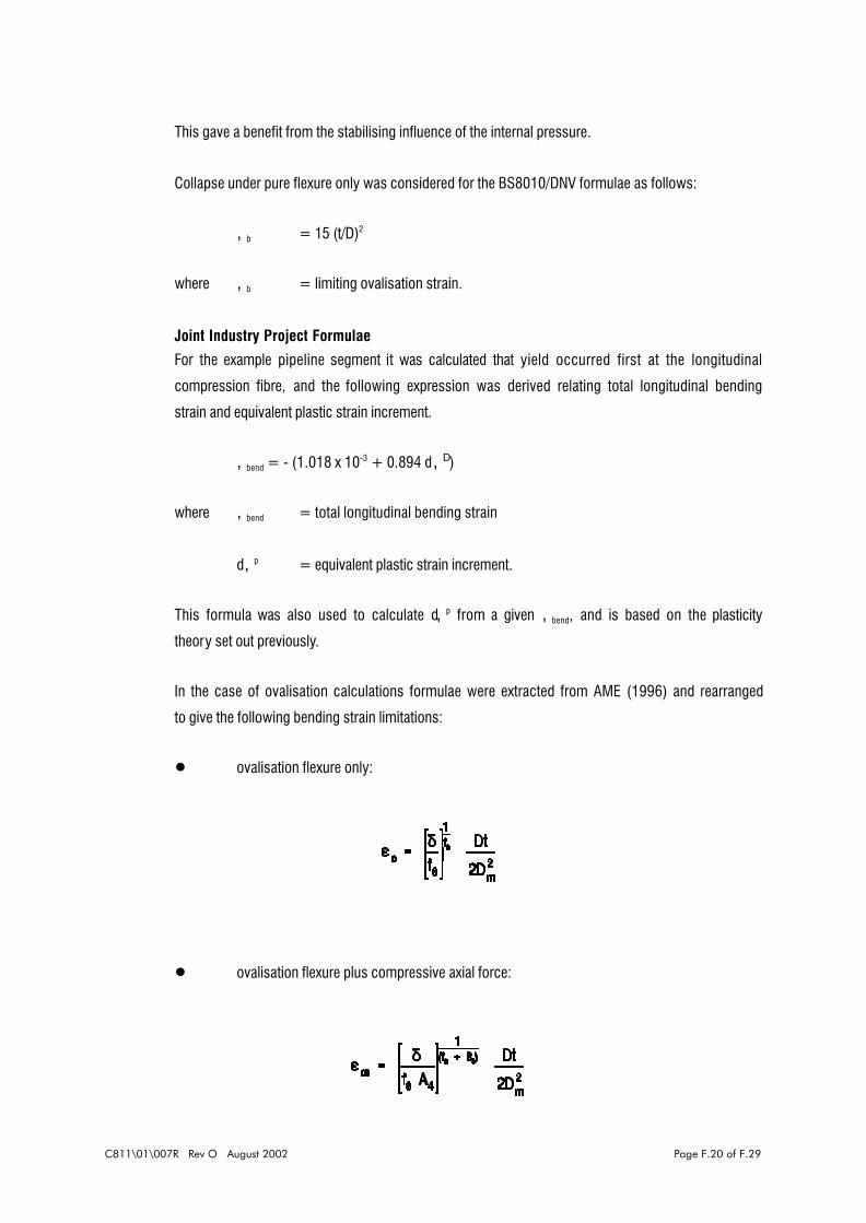
C811\01\007R Rev O August 2002 Page F.20 of F.29
This gave a benefit from the stabilising influence of the internal pressure.
Collapse under pure flexure only was considered for the BS8010/DNV formulae as follows:
,b = 15 (t/D)2
where ,b = limiting ovalisation strain.
Joint Industry Project Formulae
For the example pipeline segment it was calculated that yield occurred first at the longitudinal
compression fibre, and the following expression was derived relating total longitudinal bending
strain and equivalent plastic strain increment.
,bend = - (1.018 x 10⁻³ + 0.894 d,D)
where ,bend = total longitudinal bending strain
d,p = equivalent plastic strain increment.
This formula was also used to calculate d,p from a given ,bend, and is based on the plasticity
theory set out previously.
In the case of ovalisation calculations formulae were extracted from AME (1996) and rearranged
to give the following bending strain limitations:
! ovalisation flexure only:
! ovalisation flexure plus compressive axial force:
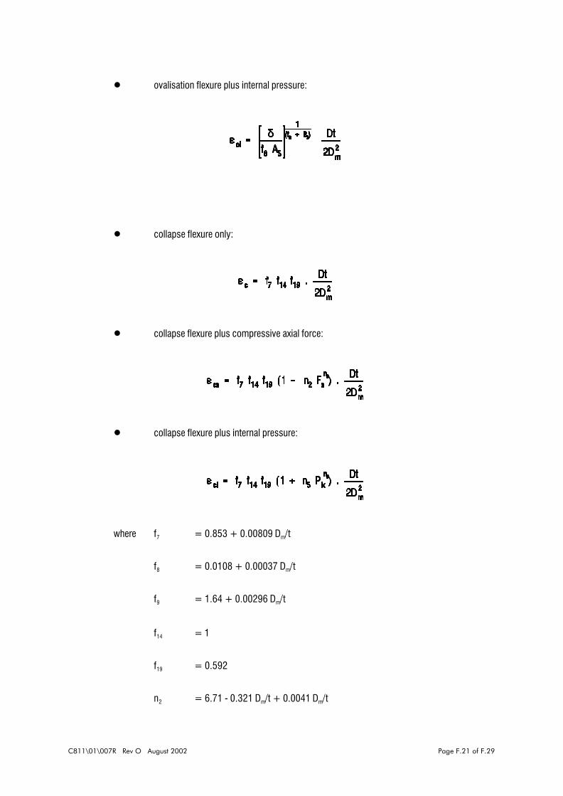
C811\01\007R Rev O August 2002 Page F.21 of F.29
! ovalisation flexure plus internal pressure:
! collapse flexure only:
! collapse flexure plus compressive axial force:
! collapse flexure plus internal pressure:
where f7 = 0.853 + 0.00809 Dm/t
f8 = 0.0108 + 0.00037 Dm/t
f9 = 1.64 + 0.00296 Dm/t
f14 = 1
f19 = 0.592
n2 = 6.71 - 0.321 Dm/t + 0.0041 Dm/t

C811\01\007R Rev O August 2002 Page F.22 of F.29
n3 = 2.33 - 0.036 Dm/t
n5 = 1.98
n6 = 1.28
A4 = 1 + 0.0258 Fa + 2.32 Fa2
B4 = 0.0637 Fa + 0.946 Fa2
A5 = 1 - 1.2 Pix + 0.401 Pix2
B5 = - 1.15 Pix + 0.736 Pix2
Fa = Fco / (BFoDmt)
Pix = (p i - pa) / Piy
Dm = pipe median diameter
Fo = material yield strength
Fco = axial force in pipe wall
pi = internal pressure
pa = external pressure
Piy = Fo (2t/D) for D/t > 20
= Fo (D2 - Di
2) /(D2 + Di2) for D/t # 20
D = pipe outside diameter
Di = pipe inside diameter
F.1.5.3 Results from ComparisonThe results of all the strain calculations are summarised in Table F.1.5. Strain limits are given
for the criteria indicated and the two sets of formulae. Total bending strain and equivalent
C811\01\007R Rev O August 2002 Page F.23 of F.29
plastic strain increment are given in per cent.
In comparing the bending strain limits it is seen that, for obvious reasons, first yield and 0.1%
equivalent plastic strain set the lowest limits. For the AME formulae the 1% ovalisation limit is
always less than the corresponding collapse limit. The opposite of this is true for the
BS8010/DNV formulae, where only the flexure-only results may be compared between these two
criteria.
The effects of axial force in the case of the AME formulae are seen to reduce the strain limits
from the pure flexure ones; the reduction is negligible in the case of the ovalisation limit, but is
larger in the collapse case. The beneficial effects of internal pressure, in terms of increased
limits from those set by pure flexure, are shown by the AME formulae; the limit is very nearly
doubled in the case of the collapse criterion. Similar gains are shown by the BS8010/DNV
formulae in the case of ovalisation.
Generally the AME limits are more onerous than those set by BS8010/DNV in the case of
ovalisation, but allow larger limiting strains for the collapse criterion.
F.1.6 CLOSING REMARKS
Criteria are available from existing pipeline design codes and guidelines for determining the
static strength of pipeline spans. It is broadly agreed that the criteria from these sources are
overly conservative and very limited in their scope.
BS8010, for example, sets the equivalent plastic strain increment as 0.1% plus other material
requirements af ter high straining. Indications are, however, that strains of up to 5% can be
tolerated in X52 and X46 pipeline materials without undermining their safety (OTN 94 186, 1994).
Whilst this would represent a large step change in term of material limitation, it does throw more
emphasis onto the criteria set by, for example, ovalisation and section collapse which tend to
set limits in excess of the 0.1% plastic strain increment criterion, but much less than a 5% total
strain limit.
Some formulations are available in the codes/guidelines for ovalisation and local buckling
calculations but these do not cover the whole range of force combinations that a pipeline span
is subject to. The JIP work (AME, 1996) represents the most comprehensive approach to date
in terms of the influence of load combinations on ovalisation and section collapse. This too has
its limitations insofar as it covers loadings combining flexure with pressure or axial force in
pairs, but does not deal with flexure, axial force and pressure acting simultaneously.

C811\01\007R Rev O August 2002 Page F.24 of F.29
Nevertheless it would be extremely useful to extract from the JIP report a subset of criteria
relevant to pipeline spanning and to develop the strain limitations across the full range of
pipelines in Amoco's North Sea operations, as a precursor to investigating the effects these
have on allowable span length.
F.1.7 REFERENCES
1. AME (1996). 'Establishment of strain-based criteria and analysis for the assessment
of subsea pipelines. Final report'. Project Review Report AME/26563/R/04, August
1996.
2. BS8010: Part 3 (1993). 'Code of Practice for Pipelines. Part 3. Pipelines subsea:
design, construction and installation'. BSI 1993.
3. Det Norse Veritas (DNV) : 1981 (Reprint with corrections 1982). Rules for Submarine
Pipeline Systems.
4. OTN 94 186 (1994). 'Investigation of structural and material implications of bending
pipelines to large strains'. Offshore Technology Report OTN 94 186. Commercial in
Confidence PEN/K/3066, September 1994.

C811\01\007R Rev O August 2002 Page F.25 of F.29
BS8010 DNV B31.8 B31.4 DEnGN IP6
a Acceptable conditions T T ? x x x
b Strain limits ? ? x x x x
c Buckling T ? x x x x
d Ovalisation ? ? x x x x
e Cumulative plastic strain x T x x x x
f Out-of-straightness x x x x x x
g Material properties T T x x x x
h Welded sections ? ? x x x x
I Testing T T x x x x
j Low cycle fatigue x x x x x x
k Availability of strain-
based criteria
? ? x x x x
Key: x = No detail to poorly detailed coverage
? = Poorly detailed to partly detailed coverage
T = Partly detailed to well detailed coverage
* = Well detailed to explicitly detailed coverage
Table F.1.1 Coverage detail of strain-based assessment in codes reviewed in OTN 94 186 (1994)

C811\01\007R Rev O August 2002 Page F.26 of F.29
BS8010 DNV B31.8 B31.4 DEnGN IP6 RP1111
a Acceptable conditions T T ? x x x ?
b Strain limits ? ? x x x x x
c Buckling T ? x x x x ?
d Ovalisation ? ? x x x x x
e Cumulative plastic strain x T x x x x x
f Out-of-roundness x x x x x x x
g Material properties T T x x x x x
h Welded sections ? ? x x x x ?
I Testing T T x x x x x
j Low cycle fatigue x x x x x x x
k Availability of strain-
based criteria
? ? x x x x x
Key: x = No detail to poorly detailed coverage
? = Poorly detailed to partly detailed coverage
T = Partly detailed to well detailed coverage
* = Well detailed to explicitly detailed coverage
Table F.1.2 Coverage detail of strain-based assessment in AME (1996) [As Table 3.1, but updated to
include RP 1111]

C811\01\007R Rev O August 2002 Page F.27 of F.29
Pipe outside diameter D 762 mm
Pipe wall thickness t 17.5 mm
Steel Young's modulus E 207 GPa
Steel Poisson's ratio < 0.3
Steel yield strength Fo 358 MPa
Steel coefficient of thermal expansion " 1.16x10⁻⁵ //C
Maximum internal operating pressure pi 9 MPa
Contents temperature 2i 38 /C
Minimum water depth at LAT d 28m
Local seawater density Dw 1025 kg/m3
Local seawater temperature 2a 8 /C
Table F.1.3 Pipeline data

C811\01\007R Rev O August 2002 Page F.28 of F.29
External pressure on pipe pa 0.281 MPa
Net internal pressure on pipe pico 8.719 MPa
Hoop stress F2 185.5 MPa
Prebending longitudinal stress Fxo -16.4 MPa
Prebending longitudinal force Fco -0.671 MN
Longitudinal yield force Faco 14.65 MN
Internal yield pressure Piy 16.4 MPa
Elastic buckling pressure Pe 5.5 MPa
Table F.1.4 Pipeline results (full axial fixity assumed)
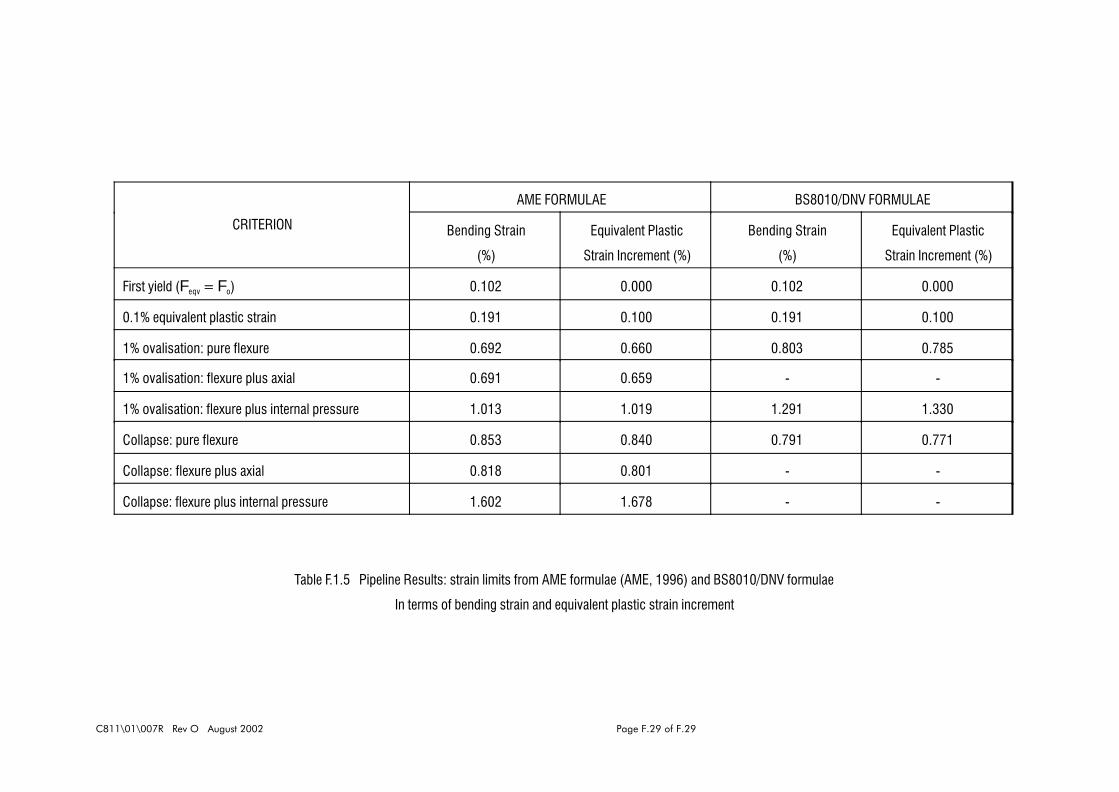
C811\01\007R Rev O August 2002 Page F.29 of F.29
CRITERION
AME FORMULAE BS8010/DNV FORMULAE
Bending Strain
(%)
Equivalent Plastic
Strain Increment (%)
Bending Strain
(%)
Equivalent Plastic
Strain Increment (%)
First yield (Feqv = Fo) 0.102 0.000 0.102 0.000
0.1% equivalent plastic strain 0.191 0.100 0.191 0.100
1% ovalisation: pure flexure 0.692 0.660 0.803 0.785
1% ovalisation: flexure plus axial 0.691 0.659 - -
1% ovalisation: flexure plus internal pressure 1.013 1.019 1.291 1.330
Collapse: pure flexure 0.853 0.840 0.791 0.771
Collapse: flexure plus axial 0.818 0.801 - -
Collapse: flexure plus internal pressure 1.602 1.678 - -
Table F.1.5 Pipeline Results: strain limits from AME formulae (AME, 1996) and BS8010/DNV formulae
In terms of bending strain and equivalent plastic strain increment
C811\01\007R Rev O August 2002 Page G.0.1 of G.0.3
APPENDIX G
RECOMMENDED INSPECTION
STRATEGY
C811\01\007R Rev O August 2002 Page G.0.2 of G.0.3
TABLE OF CONTENTS
Page No
G.1
G.2
G.3
PROPOSED IRM STRATEGY
G.1.1 SUMMARY
G.1.2 SYSTEM DEFINITION
G.1.3 STAGE 1: INITIAL ANALYSIS
G.1.4 STAGE 2: PROPOSED INSPECTION AND MAINTENANCE SCHEDULE
G.1.5 STAGE 3: UPDATED ANALYSIS
INPUT REQUIRED
G.2.1 SUMMARY
G.2.2 PIPELINE DATA
G.2.3 DEFINITION OF PIPELINE FAILURE MODES, LIMIT STATES AND TARGET
RELIABILITIES
G.2.4 PROBABILITY ANALYSIS
G.2.4.1 Assessment of hazard likelihood of occurrence
G.2.4.2 Failure models
G.2.4.3 Basic variable statistics
G.2.4.4 Component and system reliability analysis
G.2.5 CONSEQUENCE MODELS
G.2.5.1 Fire and blast analysis results
G.2.5.2 Economic considerations
G.2.5.3 Life-safety considerations
G.2.6 INSPECTION METHODS, COSTS AND MEASUREMENT UNCERTAINTY
G.2.7 MAINTENANCE AND REPAIR METHODS, AND COSTS
REFERENCES

C811\01\007R Rev O August 2002 Page G.0.3 of G.0.3
LIST OF TABLES
Table G.1.1 'Acceptable' failure probabilities (for design) from the SUPERB project [31]
LIST OF FIGURES
Figure G.1.2 Illustrative variation of predicted reliability index with time for a single failure mode
Figure G.1.3 Years to next inspection
Figure G.1.4 Illustrative variation of evaluated reliability index with time throughout pipeline life
Figure G.1.5 Flowchart for STAGE 1 : Initial analysis
Figure G.1.6 Flowchart for STAGE 2 : Propose and assess IRM schedule (Preposterior analysis)
Figure G.1.7 Flowchart for STAGE 3 : Update analysis based on inspection results (Posterior
analysis)
Figure G.2.1 Illustration of the joint failure point for the intersection of two events
C811\01\007R Rev O August 2002 G.1.1 of G.1.26
G.1 PROPOSED IRM STRATEGY
G.1.1 SUMMARY
This appendix outlines a risk and reliability-based integrity management system to optimise
planning strategy for application to pipeline inspection. The strategy considers both:
! the long term reliability of the pipeline system to ensure that confidence in the
integrity of the pipeline is maintained, and
! cost-based risk so that the expected costs of alternative inspection schemes can
be compared and minimised on a rational basis.
The proposed strategy is generic in nature, flexible and modular. The strategy can be applied
to major transmission lines as well as infield lines, and the methodology can be applied to
platform pipework, risers and spool pieces, as well as subsea pipelines. Statutory, Company,
or Asset Manager inspection requirements can be readily included in the procedure. A
preliminary assessment or ‘first-pass’ can be undertaken with simple engineering models and
published/existing company data, and once critical areas have been identified, more
sophisticated models and analysis techniques can be used to improve the assessment. The
basic methodology is modular so that future analysis techniques, data and knowledge can be
incorporated.
The strategy is based on structural reliability theory which is widely recognised as providing a
rational basis for a decision process. Application of reliability techniques enables an appropriate
and organised treatment of uncertainties and thus facilitates a consistent assessment of the
safety and serviceability of the pipeline.
Essentially, there are three main stages to the strategy which are aimed at the following
questions:
i. What is the present state of the pipeline? (Initial analysis)
ii. How do we plan for the future? (Inspection schedule preparation)
iii. How do we monitor the state of the pipeline and update the plan when new
information becomes available? (Schedule updating)
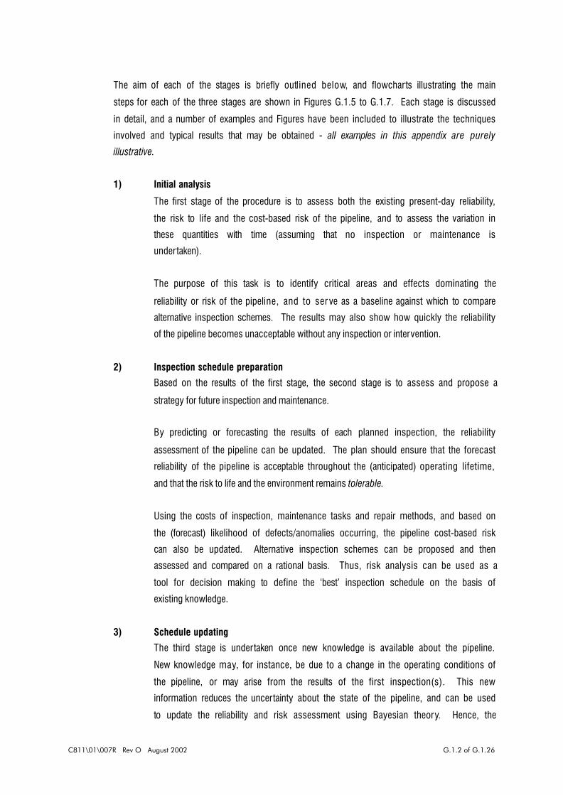
C811\01\007R Rev O August 2002 G.1.2 of G.1.26
The aim of each of the stages is briefly outlined below, and flowcharts illustrating the main
steps for each of the three stages are shown in Figures G.1.5 to G.1.7. Each stage is discussed
in detail, and a number of examples and Figures have been included to illustrate the techniques
involved and typical results that may be obtained - all examples in this appendix are purely
illustrative.
1) Initial analysis
The first stage of the procedure is to assess both the existing present-day reliability,
the risk to life and the cost-based risk of the pipeline, and to assess the variation in
these quantities with time (assuming that no inspection or maintenance is
undertaken).
The purpose of this task is to identify critical areas and effects dominating the
reliability or risk of the pipeline, and to ser ve as a baseline against which to compare
alternative inspection schemes. The results may also show how quickly the reliability
of the pipeline becomes unacceptable without any inspection or intervention.
2) Inspection schedule preparation
Based on the results of the first stage, the second stage is to assess and propose a
strategy for future inspection and maintenance.
By predicting or forecasting the results of each planned inspection, the reliability
assessment of the pipeline can be updated. The plan should ensure that the forecast
reliability of the pipeline is acceptable throughout the (anticipated) operating lifetime,
and that the risk to life and the environment remains tolerable.
Using the costs of inspection, maintenance tasks and repair methods, and based on
the (forecast) likelihood of defects/anomalies occurring, the pipeline cost-based risk
can also be updated. Alternative inspection schemes can be proposed and then
assessed and compared on a rational basis. Thus, risk analysis can be used as a
tool for decision making to define the ‘best’ inspection schedule on the basis of
existing knowledge.
3) Schedule updating
The third stage is undertaken once new knowledge is available about the pipeline.
New knowledge may, for instance, be due to a change in the operating conditions of
the pipeline, or may arise from the results of the first inspection(s). This new
information reduces the uncertainty about the state of the pipeline, and can be used
to update the reliability and risk assessment using Bayesian theory. Hence, the

C811\01\007R Rev O August 2002 G.1.3 of G.1.26
inspection schedule can be redefined for the remaining life of the pipeline.
Thus, although initially a full inspection schedule is produced, it may only be the first
inspection that is carried out to plan. The schedule for the remaining life of the
pipeline is updated based on the best available information at the time, and
consequently a number of schedules may be produced at intervals throughout the life
of the system.
G.1.2 SYSTEM DEFINITION
The first task is to split the pipeline into zones or segments with common attributes; that is:
! hazards,
! failure modes,
! failure consequences, and
! inspection methods.
A typical zoning scheme for a transmission pipeline might be:
i. platform pipework;
ii. above water riser - from the topside ESD valve to MSL;
iii. below water riser - from MSL to the spool piece/riser flange;
iv. the spool piece;
v. subsea pipeline in platform safety zone (within 500m of the platform);
vi. mid-line or open water pipeline;
vii. shore zone;
viii. land pipeline.
Each zone can then be analysed individual ly, and an inspection and maintenance schedule
could be defined for each zone. Alternatively, the approach is flexible enough that the reliability
and risk results for a number of zones can be compared and combined to define inspection
schedules for larger segments of the pipeline, or for one schedule encompassing the whole
pipeline. (However, lumping failure consequences together for different zones may not lead to
the most economic solution.)
C811\01\007R Rev O August 2002 G.1.4 of G.1.26
G.1.3 STAGE 1: INITIAL ANALYSIS
Step 1.1 Identify hazards, failure modes and limit states
For each pipeline zone, the first step is to identify all of the hazards that can affect the integrity
and operation of the pipeline.
It is important that all of the hazards are identified since the omission of a hazard will mean that
the study will be incomplete, and the resulting inspection schedule may not be capable of
detecting a potential failure mechanism in time.
For each hazard the potential failure modes need to be identified, and these need to be linked
with limit states.
A number of definitions for the limit states for operating pipelines have been proposed. One of
the most popular definitions, which has been adopted by the SUPERB project (for Submarine
Pipeline Reliability Based Design Guideline) [1, 2], is based on four limit states which are
defined as follows.
The Serviceability Limit State (SLS) requires that the pipeline must be able to remain
in service and operate normally (although the integrity may be impaired), and includes
the following modes:
- yielding;
- section ovalisation which prevents pigging;
- ratcheting;
- loss of concrete coating.
The Ultimate Limit State (ULS) generally corresponds to the maximum load bearing
capacity criteria, and includes the following failure modes:
- bursting;
- buckling;
- plastic collapse;
- unrestrained plastic flow;
- unstable fracture;
- tensile rupture.
The Fatigue Limit State (FLS) results from excessive fatigue crack growth and damage
accumulation under cyclic loading. This is an ULS referring to the entire life time of
the pipeline.
The Accidental Limit State (ALS) corresponds to ultimate failure due to accidental

C811\01\007R Rev O August 2002 G.1.5 of G.1.26
loads and/or local damage of the pipeline with loss of structural integrity and r upture.
The limit states are used in the definition of target reliabilities (Step 1.2). Alternative definitions
for limit states may be adopted with appropriate targets.
When it comes to assessing the likelihood of a hazard occurring (Step 1.3), it may be helpful
to identify both the event initiating each hazard and the possible effects that may be caused.
For example, an event initiation due to a trawl beam impact may lead to weight coat damage,
anode damage, pipe denting, gouging, or rupture.
It is also useful to identify whether the hazard leads to a failure mode which is instantaneous
or whether it leads to a mode which affects the long term integrity of the pipeline.
! Hazards leading to instantaneous failure generally affect the Accidental Limit State,
and include: dropped objects, dragged anchors, and severe trawl beam impacts.
! Hazards which are solely a time-varying effect leading to the long term degradation
of the pipeline include: external and internal corrosion, erosion, and fatigue.
! Hazards which may be both include gouging due to trawl beam impact leading
potentially to instantaneous rupture or to a stress-raiser for fatigue. Scour leading
to pipeline spanning is also a hazard that may lead either to very rapid failure if the
span and wave and current conditions are such that severe cross flow vortex
shedding ‘locks-on’, or if the vibration is less serious and occurs infrequently it
may lead to fatigue degradation.
Step 1.2 Assess target reliabilities
For each pipeline zone and limit state, the next step is to assess an acceptable target reliability.
An assessment of the target reliability(s) should consider the actual consequences and nature
of failure, economic losses and the potential for human injury or environmental pollution. Ideal ly,
targets should be calibrated with well-established designs that are known to have adequate
safety, and actual failure statistics are useful in the assessment if interpreted carefully.
A number of organisations have proposed target reliabilities for use in the absence of better
information for a wide variety of structures, including offshore platforms and pipelines. For
submarine pipelines, the most recent and comprehensive assessment has been undertaken as
par t of the SUPERB project, and their target failure probabilities are shown in Table G.1.1. (It
should be noted that appropriate units have to be considered to ensure system safety).

C811\01\007R Rev O August 2002 G.1.6 of G.1.26
SUPERB’s proposed targets for the various limit states are based on the safety class of the
pipeline zone. A low safety class corresponds to a pipeline conveying nonflammable water-
based products (ie not a Major Accident Hazard Pipeline); a high safety class corresponds to
the (subsea) sections of oil or gas pipelines within the platform safety zone, ie within 500m of
the platform; and the normal safety class corresponds to oil or gas pipelines in open water.
The SUPERB targets were primarily developed for the design of new submarine pipelines and
they may not be directly applicable to the reassessment of existing pipelines. Never theless,
they offer a very useful reference point.
Limit State
Category
Safety Class
Low Normal High
Serviceability (SLS) 10-1 - 10-2
(per year)
10-2 - 10-3
(per year)
10-2 - 10-3
(per year)
Ultimate (ULS) 10-2 - 10-3
(per year)
10-3 - 10-4
(per year)
10-4 - 10-5
(per year)
Fatigue (FLS) 10-3
(per lifetime)
10-4
(per lifetime)
10-5
(per lifetime)
Accidental (ALS) 10-4
(per km per year)
10-5
(per km per year)
10-6
(per km per year)
Table G.1.1 ‘Acceptable’ failure probabilities (for design) from the SUPERB project [31]
Step 1.3 Assess likelihood of each hazard and probability of failure
For each hazard or potential cause of failure, the next step is to estimate the probability of
exceedence for each relevant limit state.
For a preliminary assessment, generic databases of pipeline failures can be used; the most
recent and comprehensive database for North Sea pipelines and risers is PARLOC (Pipeline and
Riser Loss of Containment study) [3]. PARLOC is based on data relating to 17,245km of
pipelines since 1975, and can be used to assess the likely loss of containment frequency due
to different failure causes in the various pipeline or riser zones, depending on the pipeline type,
diameter, length, contents, and age.
Whilst generic data is acceptable for a prel iminar y assessment, these data must be used with
care since the particular circumstances of failure incidents may not be known. In addition, the
PARLOC database at least, does not record the inspection and maintenance systems for the
incidents.

C811\01\007R Rev O August 2002 G.1.7 of G.1.26
More detailed analyses related to a specific pipeline can be undertaken by assessing the
likelihood of a hazard or cause of failure occurring, and then evaluating the probability of failure
given that the hazard scenario has occurred. Thus, the probability of failure due to a hazard
is evaluated from:
(G.1.1)
where is the likelihood of a hazard occurring per year per km,
and is the probability of failure of the pipeline given that the hazard has occurred.
For some hazards it is almost cer tain that they are likely to occur, ie , for instance
internal corrosion and fatigue. For other hazards the likelihood of occurrence can be based on
subjective judgement, historical records, or by a detailed assessment of all of the relevant data.
For example:
! trawling hazards can be assessed by studying historical records of fishing activity
in the area, and the depth and extent of burial/exposure of the pipeline;
! the likelihood of a dropped container hitting the pipeline can be assessed from the
number of seaboard movements made by the platform crane per year, crane failure
rate statistics, and by using hydrodynamic analysis of a free-falling object to
assess the probability of hitting the pipeline on the seabed.
It is also necessary to estimate or evaluate the probability that the pipeline will exceed the limit
state criterion under the scenario that a hazard has occurred, ie . For a preliminary
‘first-pass’ analysis a subjective assessment may be made; for a more detailed assessment
structural reliability methods may be used, which may be made as sophisticated as necessary.
The main requirements for undertaking a structural reliability analysis are:
! an analytical model for assessing exceedence of the limit state criterion, this is
known as the failure function;
! an assessment of the natural variability and uncertainty of all of the parameters
influencing the failure criterion.
At its simplest, a failure function, Z, can be defined as:
(G.1.2)

C811\01\007R Rev O August 2002 G.1.8 of G.1.26
where R is the strength or strength effect,
and S is the load or load effect.
R and S, and/or Z may of course be complicated functions. For all of the main failure modes
adequate failure functions can be formed from the deterministic analysis models presently used
in assessment. More sophisticated models can be substituted if necessary.
The (annual) probability of failure due to a failure mode or hazard i, , is given by:
(G.1.3)
where is the probability density function for the basic variables.
There are basically three main types of uncer tainty that are relevant and which should be
included in the analysis, these are:
i. Physical uncertainty which is due to the natural variability of the input quantities,
such as: SMYS, wall thickness, ovalisation, wave and current velocity parameters,
span length etc.;
ii. Statistical uncertainty which arises from the uncertainty in estimating the
parameters of the probability distributions due to limited data;
iii. Model uncertainty which arises from the idealisations and inaccuracies of the
engineering models used to predict loading and resistance.
A number of well-researched techniques have been developed for undertaking structural
reliability analysis, including first and second order methods (FORM/SORM), and a variety of
Monte Carlo simulation approaches.
The failure probability may be defined on an annual basis or for some other reference period
depending on how the failure function and the basic variables, and the likelihood of occurrence,
are defined. When probabilities of failure are compared with target probabilities it is clearly
impor tant that they are compared on a consistent basis, that is annual targets with annual
probabilities, lifetime with lifetime, etc.
Step 1.4 Evaluate system failure probability
For each failure mechanism, for example cross-flow vortex shedding due to spanning, the failure

C811\01\007R Rev O August 2002 G.1.9 of G.1.26
probabilities for each span are then combined to evaluate the total failure probability for the
pipeline zone (or for the whole pipeline). Then for each limit state the system probability is
derived by combining the failure probabilities for each failure mechanism.
Pipelines can be considered to be series systems, since the failure of any one par t due to any
failure mode is failure of the system. Thus, strictly the union of the probabilities for each failure
event should be computed. Simple bounds on the system probability may be evaluated as:
(G.1.4)
In practice the bounds are likely to be too wide for practical use. However, they can be
improved by judging the likely correlation between the events. Thus, for events which are highly
correlated, for instance general corrosion between one section and the next, the combined
probability will be dominated by the maximum individual failure probability.
For highly correlated events: (G.1.5a)
However, for different failure modes and hazards most of the failure events will be largely
uncorrelated, and a reasonable and conservative estimate can be obtained by evaluating and
combining the probabilities for the individual events thus:
For largely uncorrelated events: (G.1.5b)
Step 1.5 Evaluate time-varying probability
Based on estimates of corrosion rates, scour rates, crack growth, etc., the reliability analysis
can be repeated to assess the likely deterioration in reliability with time by undertaking the
analysis at yearly (or more frequent) intervals. The uncertainty in predicted corrosion rates,
scour rates, etc., should of course be included in the reliability analysis; the uncertainty in these
rates is one of the main reasons for undertaking inspections.
The likelihoods and failure probabilities for most of the events affecting the Accidental Limit
State are, or can be assumed to be, constant from year-to-year. However, this is not so for
most of the events affecting the other limit states.

C811\01\007R Rev O August 2002 G.1.10 of G.1.26
The variation in system probability with time can then be evaluated using Eqns (G.1.5a) or
(G.1.5b) for each time interval.
Step 1.6 Reliability-based assessment
At this stage, for each limit state it is possible to plot the variation in (annual) failure probability
and/or reliability index against time, and to compare these with the target probabilities or
equivalent reliability indices.
On the same plots it is also useful to show curves for each of the contributing failure hazards
and/or failure modes. This gives a graphical indication of the most dominant failure modes, the
critical hazards, and indicates the time when the predicted reliability of the pipeline becomes
unacceptable.
An illustration of such a plot is shown in Figure G.1.1. In the Figure, failure modes 1 and 2 show
little or no deterioration in reliability with time. Initially failure mode 3 is the least likely to occur,
however af ter 5 years this mode dominates the system reliability and leads to a rapid fall in
reliability. The reliability becomes unacceptable af ter 12 years in this example, indicating that
an inspection is necessary before this time.
0 5 10 15 20
Time
Relia
bilit
y
Mode 1
Mode 2
Mode 3
System
Target
Figure G.1.1 Illustrative variation in reliability for different failuremodes with time

C811\01\007R Rev O August 2002 G.1.11 of G.1.26
Step 1.7 Assess consequences of failure
For a risk-based assessment it is necessary to assess the consequences of failure. Depending
on the contents and pressure of the pipeline, and the type and location of the failure, the
consequences may be purely economic, they may involve environmental damage, and/or they
may lead to injury and / or loss of life.
For mid-line or open water pipelines, and for all zones of pipelines to / from unmanned platforms,
the consequences of failure are largely economic.
The cost of failure of a pipeline is likely to include:
! loss of production,
! non-delivery penalty charges,
! loss of product,
! environmental pollution clean-up/mitigation,
! legal fees/fines,
! negative publicity,
! equipment damage,
! property damage.
For most pipelines the majority of the cost associated with a mid-line failure may be associated
with lost production which can be readily assessed. For shared lines, non-delivery penalty
charges are also likely to be significant, and again these can be readily defined. The cost of
the lost product, ie the volume of product within the pipeline and lost before flow can be shut
off, can also be easily estimated.
Pollution clean-up costs relate primarily to oil flowlines; whilst it may be difficult to estimate
clean-up costs, they are unlikely to be a significant contribution to the total cost of failure.
Environmental damage may lead to negative publicity, boycotting of the operator's products etc.,
and may also lead to significant fines and increased effort and costs in securing future operating
licences. In the worst case scenario these costs are almost impossible to estimate.
For risers, sections of pipeline within the platform safety zone, and high pressure gas lines the
consequences of a pipeline rupture are more serious; they may affect the integrity of the
platform, wells and other flowlines, and may be such that human lives are put at risk. More
detailed analyses of failure scenarios may be undertaken to assess the likelihood of jet/pool
fires, flash fires, explosions, toxic clouds, etc., and to estimate their effects to the platform and
to the personnel onboard. Consequence analysis of this type is often undertaken using Event
Tree Analysis (ETA).
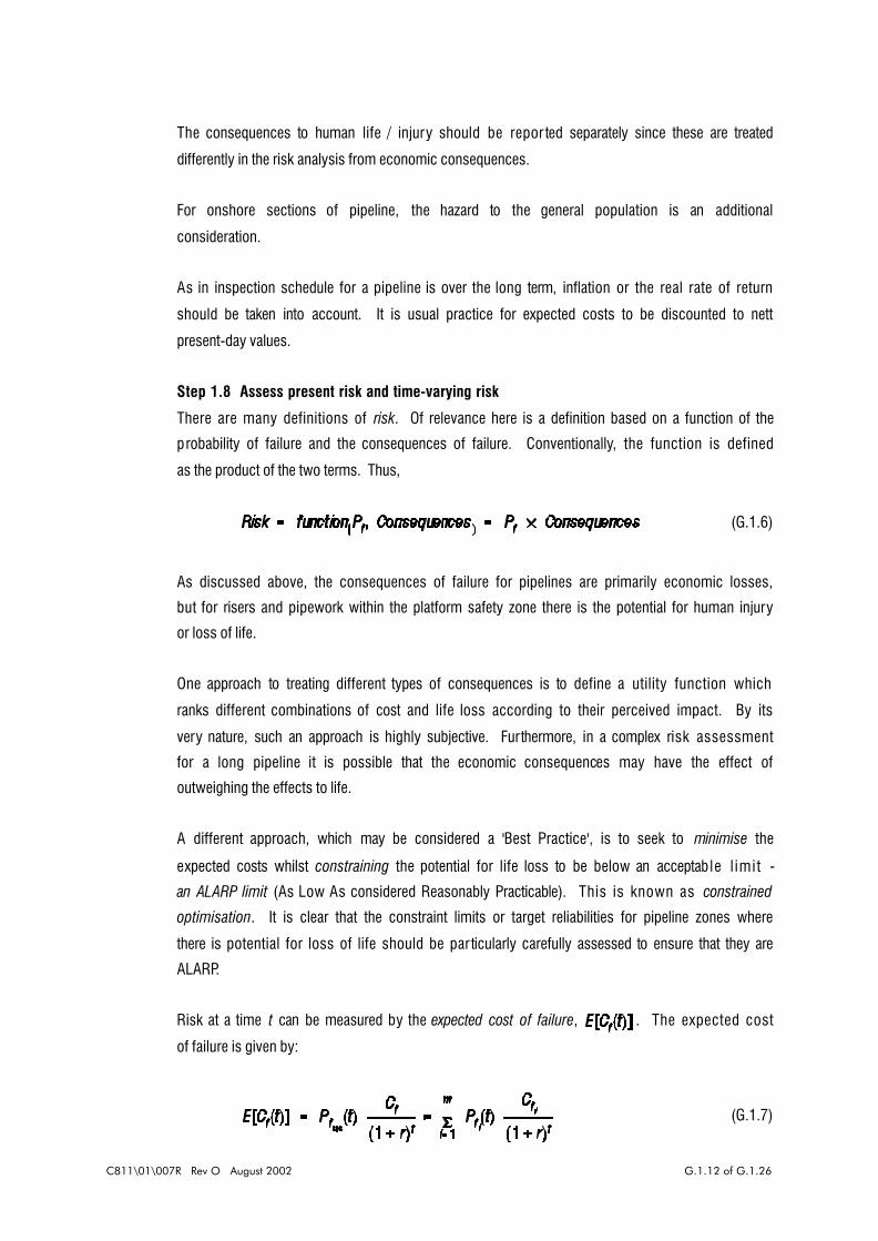
C811\01\007R Rev O August 2002 G.1.12 of G.1.26
The consequences to human life / injury should be repor ted separately since these are treated
differently in the risk analysis from economic consequences.
For onshore sections of pipeline, the hazard to the general population is an additional
consideration.
As in inspection schedule for a pipeline is over the long term, inflation or the real rate of return
should be taken into account. It is usual practice for expected costs to be discounted to nett
present-day values.
Step 1.8 Assess present risk and time-varying risk
There are many definitions of risk. Of relevance here is a definition based on a function of the
probability of failure and the consequences of failure. Conventionally, the function is defined
as the product of the two terms. Thus,
(G.1.6)
As discussed above, the consequences of failure for pipelines are primarily economic losses,
but for risers and pipework within the platform safety zone there is the potential for human injury
or loss of life.
One approach to treating different types of consequences is to define a utility function which
ranks different combinations of cost and life loss according to their perceived impact. By its
very nature, such an approach is highly subjective. Furthermore, in a complex risk assessment
for a long pipeline it is possible that the economic consequences may have the effect of
outweighing the effects to life.
A different approach, which may be considered a 'Best Practice', is to seek to minimise the
expected costs whilst constraining the potential for life loss to be below an acceptable l imi t -
an ALARP limit (As Low As considered Reasonably Practicable). This is known as constrained
optimisation. It is clear that the constraint limits or target reliabilities for pipeline zones where
there is potential for loss of life should be par ticularly carefully assessed to ensure that they are
ALARP.
Risk at a time t can be measured by the expected cost of failure, . The expected cost
of failure is given by:
(G.1.7)
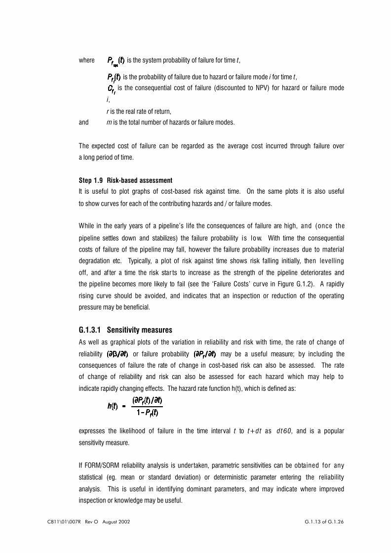
C811\01\007R Rev O August 2002 G.1.13 of G.1.26
where is the system probability of failure for time t,
is the probability of failure due to hazard or failure mode i for time t,
is the consequential cost of failure (discounted to NPV) for hazard or failure mode
i,
r is the real rate of return,
and m is the total number of hazards or failure modes.
The expected cost of failure can be regarded as the average cost incurred through failure over
a long period of time.
Step 1.9 Risk-based assessment
It is useful to plot graphs of cost-based risk against time. On the same plots it is also useful
to show curves for each of the contributing hazards and / or failure modes.
While in the early years of a pipeline’s life the consequences of failure are high, and (once the
pipeline settles down and stabilizes) the failure probability is low. With time the consequential
costs of failure of the pipeline may fall, however the failure probability increases due to material
degradation etc. Typically, a plot of risk against time shows risk falling initially, then levelling
off, and af ter a time the risk star ts to increase as the strength of the pipeline deteriorates and
the pipeline becomes more likely to fail (see the ‘Failure Costs’ curve in Figure G.1.2). A rapidly
rising curve should be avoided, and indicates that an inspection or reduction of the operating
pressure may be beneficial.
G.1.3.1 Sensitivity measuresAs well as graphical plots of the variation in reliability and risk with time, the rate of change of
reliability or failure probability may be a useful measure; by including the
consequences of failure the rate of change in cost-based risk can also be assessed. The rate
of change of reliability and risk can also be assessed for each hazard which may help to
indicate rapidly changing effects. The hazard rate function h(t), which is defined as:
expresses the likelihood of failure in the time interval t to t+dt as dt60, and is a popular
sensitivity measure.
If FORM/SORM reliability analysis is undertaken, parametric sensitivities can be obtained for any
statistical (eg. mean or standard deviation) or deterministic parameter entering the reliability
analysis. This is useful in identifying dominant parameters, and may indicate where improved
inspection or knowledge may be useful.

C811\01\007R Rev O August 2002 G.1.14 of G.1.26
G.1.4 STAGE 2: PROPOSED INSPECTION AND MAINTENANCE SCHEDULE
Step 2.1 Propose inspection and maintenance schedule
Based on a detailed assessment of the results from the first stage, a candidate inspection and
maintenance schedule can be proposed. An initial assessment of the existing inspection
schedule can be used as a comparison with other schemes, and as a basis for schedule
optimisation.
Step 2.2 Assess inspection measurement uncertainties
The measurement uncertainties associated with the proposed inspection techniques need to
be considered since each method has different capabilities for observing and reporting defects.
The inspection capabilities that need to be addressed include:
! detection limits,
! probability of detection,
! sizing accuracy,
! repeatability,
! locational accuracy.
Step 2.3 Estimate probability of maintenance or repair
Based on the estimated growth rate and the type and quali ty of the inspection planned, it is
possible to assess the probability that the defect will be so substantial that maintenance or
repair will be required. This can be evaluated using an event margin, J, which may be based
on the failure function, or may be more simply defined.
For example, for spanning the failure function, Z, may be defined in terms of frequency of
vibration, pipe stress in the span, and/or fatigue damage. However, the event margin J may be
simply defined in terms of span length.
In order to define the event margins, J, a strategy for repair needs to be proposed and defined
for each type of defect. The definition of each maintenance and repair event depends on the
type of defect.
For example, consider general corrosion. If the corrosion depth is greater than the corrosion limit
the pipeline will be derated, otherwise a corrosion inhibitor will be added. Thus, the events may
be defined as:
(G.1.8a)
(G.1.8b)

C811\01\007R Rev O August 2002 G.1.15 of G.1.26
where is the limiting depth for general corrosion,
is the predicted corrosion depth at the inspection time ,
is the measurement error associated with the inspection method.
Of course more complex margins can be defined if necessary to cover a range of options.
Step 2.4 Update reliability estimates
Using the results of the previous step, the reliability evaluated from the first stage can be
updated to account for the predicted results of the first and subsequent planned inspections -
this type of analysis may be referred to as a preposterior analysis.
For any time, t, up to the time of the first inspection, ie for , the failure probability is
evaluated as Stage 1, thus:
(G.1.9)
For any time af ter the first planned inspection, , and up to the second planned inspection, ,
ie , the failure probability is evaluated as:
= (probability of failure up to )
+ (probability of failure af ter given that the defect repair criterion is not
exceeded at )
+ (probability of failure af ter given defect found and repaired at )
That is,
(G.1.10)
where is the failure function for the pipe in the original condition,
is the failure function for the pipe af ter the defect has been repaired,
and J is the event margin (see Step 2.3)
For any time af ter the second planned inspect ion, , and up to the third planned inspection,
, ie , the failure probability is evaluated as:

C811\01\007R Rev O August 2002 G.1.16 of G.1.26
= (probability of failure up to )
+ (probability of failure af ter given defect criterion not exceeded at or )
+ (probability of failure af ter given defect found and repaired at )
+ (probability of failure af ter given defect found and repaired at )
+ (probability of failure af ter given defects found and repaired at and )
That is, (G.1.11)
As the number of planned inspections increases, the number of combinations of events
increases.
Step 2.5 Evaluate system failure probability
For each pipeline zone, and for each limit state, the probabilities can then be combined to
evaluate the system reliability. For the types of combined events discussed above it can be
difficult to evaluate the system reliabil ity accurately. However, most of the failure modes and
hazards will be largely uncorellated, and a reasonable and conservative estimate can be
obtained by combining the probabilities for the individual failure events.
Step 2.6 Reliability-based assessment
From Step 2.4, the analysis can be repeated to assess the likely deterioration in reliability with
time by undertaking the analysis for yearly (or more frequent) intervals.
An illustration of the variation of predicted reliability index with time for a single failure mode is
shown in Figure G.1.2. For the example shown in the Figure, three inspections are planned at
times , and .
Until the first planned inspection the reliability behaviour is identical to that evaluated in Stage
1. Af ter the first and each subsequent inspection the cur ve of reliability index versus time has
a marked reduction in slope. This is because the failure rate following an inspection is very
small, since:
! either a defect has not been found at all,
! or a defect has been found, measured and assessed to be ‘safe’,
! or a significant defect has been found and the pipeline has been derated or
repaired.
The extent that the predicted failure rate slope is reduced depends on the quality of the
inspection method. A poor, inaccurate and unreliable method will have little effect on the failure
rate and is of little benefit, whilst a very accurate and dependable method capable of finding and
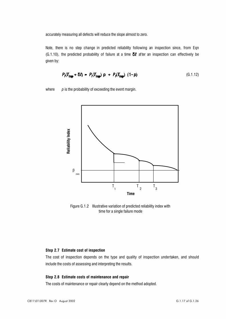
C811\01\007R Rev O August 2002 G.1.17 of G.1.26
accurately measuring all defects will reduce the slope almost to zero.
Note, there is no step change in predicted reliability following an inspection since, from Eqn
(G.1.10), the predicted probability of failure at a time af ter an inspection can effectively be
given by:
(G.1.12)
where p is the probability of exceeding the event margin.
Relia
bilit
y In
dex
Time1
T TT32
minβ
Figure G.1.2 Illustrative variation of predicted reliability index withtime for a single failure mode
Step 2.7 Estimate cost of inspection
The cost of inspection depends on the type and quality of inspection undertaken, and should
include the costs of assessing and interpreting the results.
Step 2.8 Estimate costs of maintenance and repair
The costs of maintenance or repair clearly depend on the method adopted.
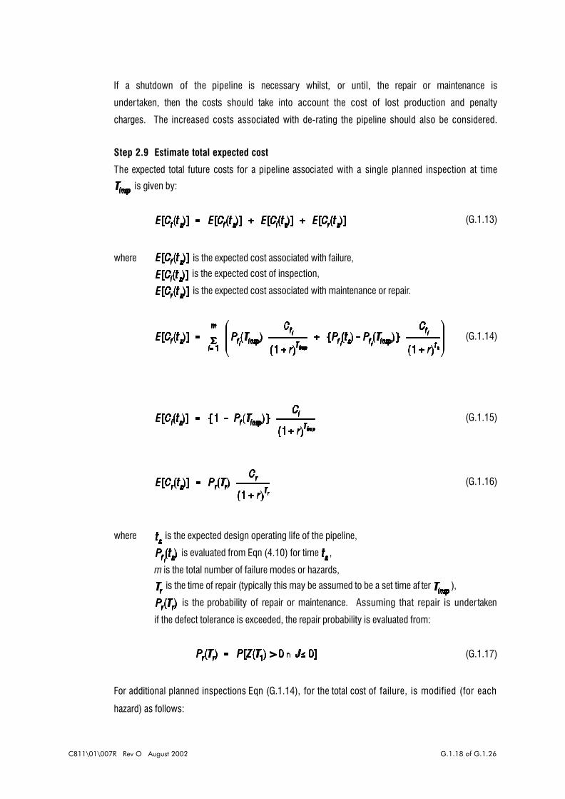
C811\01\007R Rev O August 2002 G.1.18 of G.1.26
If a shutdown of the pipeline is necessary whilst, or until, the repair or maintenance is
undertaken, then the costs should take into account the cost of lost production and penalty
charges. The increased costs associated with de-rating the pipeline should also be considered.
Step 2.9 Estimate total expected cost
The expected total future costs for a pipeline associated with a single planned inspection at time
is given by:
(G.1.13)
where is the expected cost associated with failure,
is the expected cost of inspection,
is the expected cost associated with maintenance or repair.
(G.1.14)
(G.1.15)
(G.1.16)
where is the expected design operating life of the pipeline,
is evaluated from Eqn (4.10) for time ,
m is the total number of failure modes or hazards,
is the time of repair (typically this may be assumed to be a set time af ter ),
is the probability of repair or maintenance. Assuming that repair is undertaken
if the defect tolerance is exceeded, the repair probability is evaluated from:
(G.1.17)
For additional planned inspections Eqn (G.1.14), for the total cost of failure, is modified (for each
hazard) as follows:
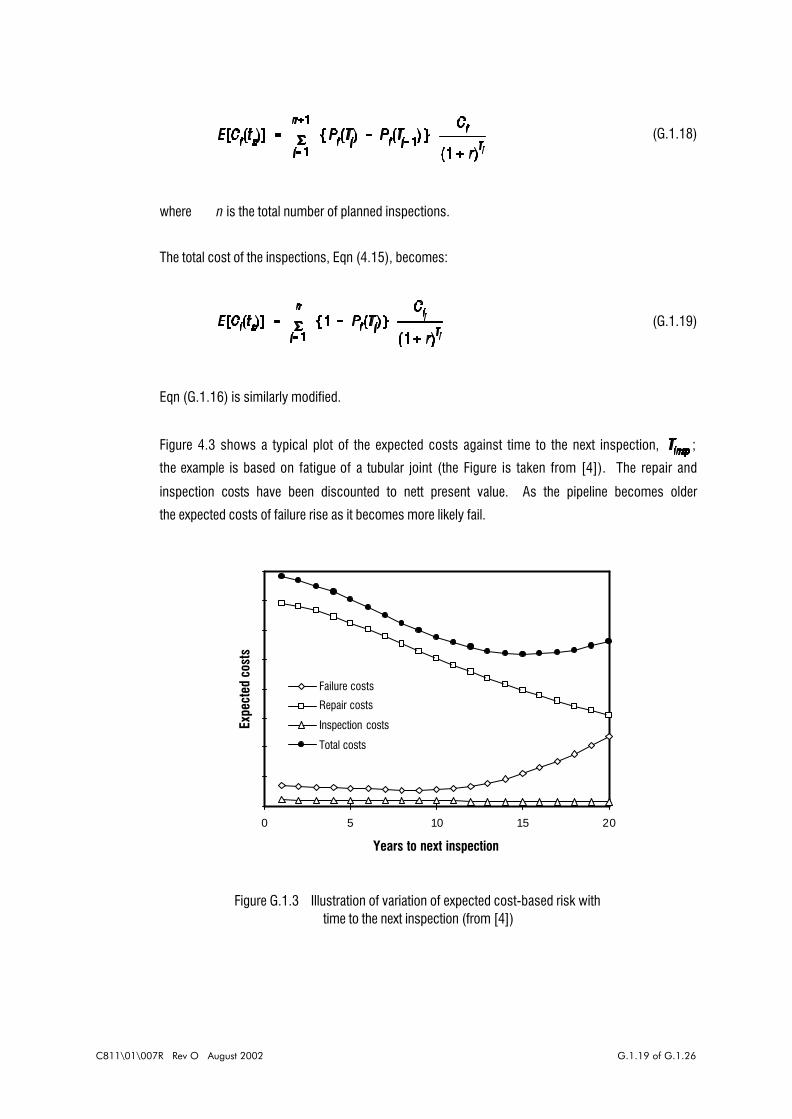
C811\01\007R Rev O August 2002 G.1.19 of G.1.26
(G.1.18)
where n is the total number of planned inspections.
The total cost of the inspections, Eqn (4.15), becomes:
(G.1.19)
Eqn (G.1.16) is similarly modified.
Figure 4.3 shows a typical plot of the expected costs against time to the next inspection, ;
the example is based on fatigue of a tubular joint (the Figure is taken from [4]). The repair and
inspection costs have been discounted to nett present value. As the pipeline becomes older
the expected costs of failure rise as it becomes more likely fail.
0 5 10 15 20
Years to next inspection
Expe
cted
cos
ts
Failure costs
Repair costs
Inspection costs
Total costs
Figure G.1.3 Illustration of variation of expected cost-based risk withtime to the next inspection (from [4])
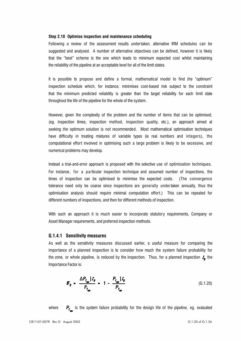
C811\01\007R Rev O August 2002 G.1.20 of G.1.26
Step 2.10 Optimise inspection and maintenance scheduling
Following a review of the assessment results undertaken, alternative IRM schedules can be
suggested and analysed. A number of alternative objectives can be defined, however it is likely
that the “best” scheme is the one which leads to minimum expected cost whilst maintaining
the reliability of the pipeline at an acceptable level for all of the limit states.
It is possible to propose and define a formal, mathematical model to find the “optimum”
inspection schedule which, for instance, minimises cost-based risk subject to the constraint
that the minimum predicted reliability is greater than the target reliability for each limit state
throughout the life of the pipeline for the whole of the system.
However, given the complexity of the problem and the number of items that can be optimised,
(eg. inspection times, inspection method, inspection quality, etc.), an approach aimed at
seeking the optimum solution is not recommended. Most mathematical optimisation techniques
have difficulty in treating mixtures of variable types (ie real numbers and integers), the
computational effort involved in optimising such a large problem is likely to be excessive, and
numerical problems may develop.
Instead a trial-and-error approach is proposed with the selective use of optimisation techniques.
For instance, for a particular inspection technique and assumed number of inspections, the
times of inspection can be optimised to minimise the expected costs. (The convergence
tolerance need only be coarse since inspections are generally under taken annually, thus the
optimisation analysis should require minimal computation effort.) This can be repeated for
different numbers of inspections, and then for different methods of inspection.
With such an approach it is much easier to incorporate statutory requirements, Company or
Asset Manager requirements, and preferred inspection methods.
G.1.4.1 Sensitivity measuresAs well as the sensitivity measures discussed earlier, a useful measure for comparing the
importance of a planned inspection is to consider how much the system failure probability for
the zone, or whole pipeline, is reduced by the inspection. Thus, for a planned inspection the
Importance Factor is:
(G.1.20)
where is the system failure probability for the design life of the pipeline, eg. evaluated

C811\01\007R Rev O August 2002 G.1.21 of G.1.26
from Eqn (G.1.9),
is the system failure probability given the planned inspection, eg. evaluated
from Eqn (G.1.10).
G.1.5 STAGE 3: UPDATED ANALYSIS
Following the results of an inspection, or a change of state of the pipeline, for instance due to
a change in operating conditions, or a as a result of a major repair to the pipeline, the inspection
schedule may be updated.
Step 3.1 Assess measurement error uncertainty
For many types of defect the results of an inspection are presented as a measurement of some
sort, eg. span length, corrosion pitting depth, etc. With any measurement there is an
associated measurement error or uncertainty which depends on the quality of the measurement
and the technique employed.
Step 3.2 Update reliability
Using the results of the previous step, along with the results from the first stage, the reliability
can be updated using Bayesian techniques.
The updated probability of failure conditioned on an inspection event is given by:
(G.1.21)
where includes the measurement uncertainty associated with the new information.
For example, consider that an inspection for internal corrosion was undertaken at time and
the measured corrosion depth was not considered large enough to warrant remedial action, ie
see Eqn (4.8a). Since the pipe has not failed at time , this information can be expressed as:
(G.1.22)
For any time af ter the first planned inspection, , and up to the second planned inspection, ,
ie , the updated failure probability is evaluated as:

C811\01\007R Rev O August 2002 G.1.22 of G.1.26
(G.1.23)
Similarly, if the measured corrosion depth was larger than the tolerance, see Eqn (4.8b), and
the pipeline was derated, this information can be expressed by:
(G.1.24)
The updated reliability is then evaluated as:
(G.1.25)
Step 3.3 Evaluate system failure probability
For each pipeline zone, and for each limit state, the probabilities can then be combined to
evaluate the updated system reliability. As before, most of the failure modes and hazards will
be largely uncorrelated, and a reasonable and conservative estimate can be obtained by
summing the probabilities for the individual failure events.
Step 3.4 Reliability-based assessment
At this stage, for each limit state it is possible to plot the variation in failure probability and/or
reliability index against time. As before, on the same plots it is useful to show curves for each
of the contributing failure hazards and/or failure modes.
Figure G.1.4 shows a typical plot of the variation in total evaluated reliability index with time
following three inspections at time , and . Af ter each inspection there is a marked rise
in reliability because of the increased knowledge and reduced uncertainty about the state of the
pipeline. The Figure also shows the effect of a repair to the pipeline following the results of the

C811\01\007R Rev O August 2002 G.1.23 of G.1.26
inspection at time - af ter the repair the reliability is restored to a similar level to the initial
condition in this case.
The effect of updating on evaluated reliability based on actual knowledge of the pipeline
contrasts with the predicted reliability based on forecast behaviour illustrated in Figure G.1.4.
Relia
bilit
y In
dex
Time
minβ
1T TT
32
Figure G.1.4 Illustrative variation of evaluated reliability index withtime throughout pipeline life
Step 3.5 Estimate cost of further inspection and maintenance
Following the results of an inspection the IRM schedule can be updated. Thus, as before the
costs of further inspections need to be estimated.
Step 3.6 Estimate total expected cost
The expected total cost for the remaining life of the pipeline following the results of an
inspection , as before, is given by:
(G.1.26)
I f fur ther inspections are planned, the expected costs can be evaluated from Eqns (G.1.14) to
(G.1.16) using the updated probabilities in-place of the predictions.
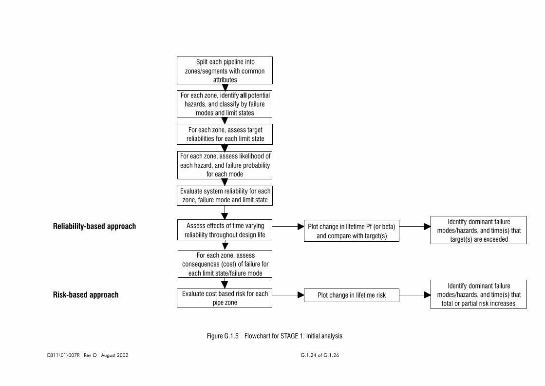
C811\01\007R Rev O August 2002 G.1.24 of G.1.26
Split each pipeline into zones/segments with common
attributes
For each zone, identify all potential hazards, and classify by failure
modes and limit states
For each zone, assess likelihood of each hazard, and failure probability
for each mode
Evaluate system reliability for each zone, failure mode and limit state
For each zone, assess target reliabilities for each limit state
Assess effects of time varying reliability throughout design life
Plot change in lifetime Pf (or beta) and compare with target(s)
Identify dominant failure modes/hazards, and time(s) that
target(s) are exceeded
For each zone, assess consequences (cost) of failure for
each limit state/failure mode
Evaluate cost based risk for each pipe zone
Plot change in lifetime riskIdentify dominant failure
modes/hazards, and time(s) that total or partial risk increases
Reliability-based approach
Risk-based approach
Figure G.1.5 Flowchart for STAGE 1: Initial analysis
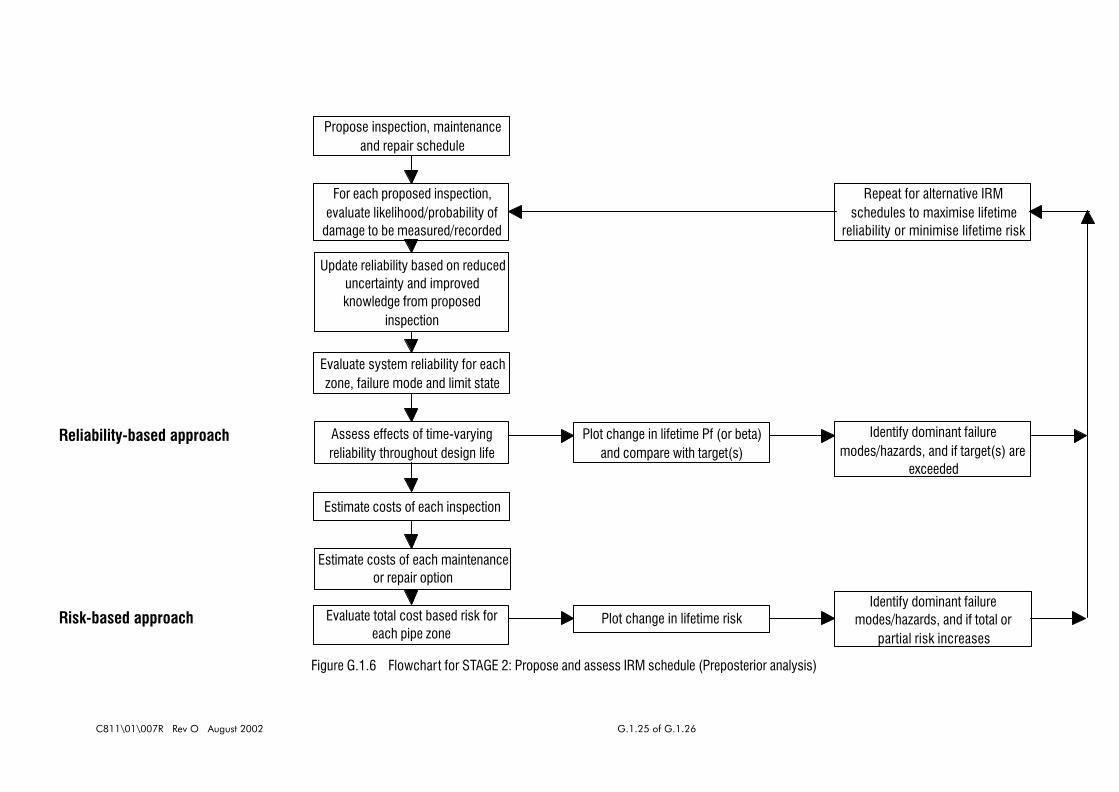
C811\01\007R Rev O August 2002 G.1.25 of G.1.26
Evaluate system reliability for each zone, failure mode and limit state
Propose inspection, maintenance and repair schedule
Assess effects of time-varying reliability throughout design life
Plot change in lifetime Pf (or beta) and compare with target(s)
Identify dominant failure modes/hazards, and if target(s) are
exceeded
Evaluate total cost based risk for each pipe zone
Plot change in lifetime riskIdentify dominant failure
modes/hazards, and if total or partial risk increases
Reliability-based approach
Risk-based approach
Estimate costs of each maintenance or repair option
Estimate costs of each inspection
For each proposed inspection, evaluate likelihood/probability of
damage to be measured/recorded
Update reliability based on reduced uncertainty and improved knowledge from proposed
inspection
Repeat for alternative IRM schedules to maximise lifetime
reliability or minimise lifetime risk
Figure G.1.6 Flowchart for STAGE 2: Propose and assess IRM schedule (Preposterior analysis)
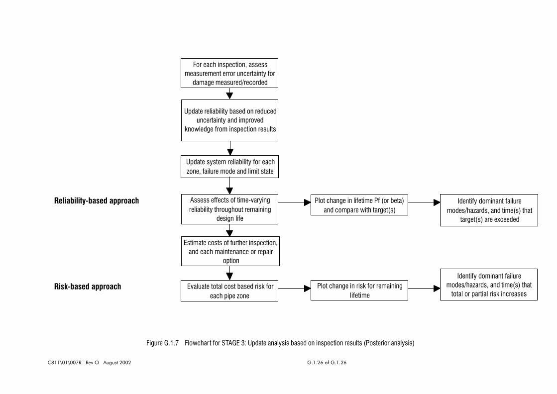
C811\01\007R Rev O August 2002 G.1.26 of G.1.26
Update system reliability for each zone, failure mode and limit state
Assess effects of time-varying reliability throughout remaining
design life
Plot change in lifetime Pf (or beta) and compare with target(s)
Identify dominant failure modes/hazards, and time(s) that
target(s) are exceeded
Evaluate total cost based risk for each pipe zone
Plot change in risk for remaining lifetime
Identify dominant failure modes/hazards, and time(s) that
total or partial risk increases
Reliability-based approach
Risk-based approach
Estimate costs of further inspection, and each maintenance or repair
option
For each inspection, assess measurement error uncertainty for
damage measured/recorded
Update reliability based on reduced uncertainty and improved
knowledge from inspection results
Figure G.1.7 Flowchart for STAGE 3: Update analysis based on inspection results (Posterior analysis)

C811\01\007R Rev O August 2002 Page G.2.1 of G.2.5
G.2 INPUT REQUIRED
G.2.1 SUMMARY
This chapter discusses the input data and analysis models that are requ ired for use with a risk
and reliability-based inspection planning procedure.
G.2.2 PIPELINE DATA
The following data are required for each pipeline:
! as-built material and geometry data, and details of pipeline coatings, anodes, etc.,
! fabrication data,
! trenching method and burial details, if any,
! soils data and seabed topography,
! metocean data along the pipeline,
! operating history and any forecast changes,
! previous inspection records,
! records of previous interventions, maintenance and repairs.
Some of the data may be incomplete, and it is important that the system should be flexible
enough to allow for this.
Results of previous analyses or assessments may be useful for comparison, and details of the
present inspection schedule should also be included.
G.2.3 DEFINITION OF PIPELINE FAILURE MODES, LIMIT STATES AND
TARGET RELIABILITIES
The failure modes and limit states need to be defined, and all of the hazards that can affect the
pipeline need to be identified. This information will be very similar for all subsea pipelines.
For each pipeline corresponding target reliabilities need to be agreed. The target reliabilities are
usually chosen to reflect the importance of the asset and the potential consequences of failure.
Targets may be defined for individual pipelines; however a more useful approach may be to
introduce a categorisation system with targets defined for each level, for example see the

C811\01\007R Rev O August 2002 Page G.2.2 of G.2.5
SUPERB targets shown in Table G.1.1.
Where life-safety is a consideration the targets should be particularly carefully defined, and the
ALARP principle should be used.
G.2.4 PROBABILITY ANALYSIS
G.2.4.1 Assessment of hazard likelihood of occurrenceFailure rate data from generic databases, such as PARLOC, are useful for preliminar y or first-
pass analyses, and such data may be useful to store as default data for use in the absence of
more specific information.
However, for more detailed analyses, the likelihood of occurrence of a hazard is required for use
with reliability analysis to evaluate the probability of failure given that a hazard has occurred.
Many hazards are almost certain to occur, eg. fatigue, corrosion, etc., and thus the likelihood
of occurrence is 1.0. For other hazards, particularly those affecting the Serviceability and
Ultimate Limit States, the likelihood may be judged subjectively, or if the results of more detailed
assessments are available these may be used instead. Likelihood data is particularly important
for the Accidental Limit State.
G.2.4.2 Failure modelsThe structural reliability analysis for the various failure modes requires accurate models to
predict failure. For the most part, the failure models may be adapted from the existing
deterministic models used for assessment.
It is anticipated that a separate module will be developed for each failure mode and/or hazard -
modules can then readily be replaced with more sophisticated models.
G.2.4.3 Basic variable statisticsThe uncertainty and variability of the basic variables also needs to be assessed. Physical,
statistical and model uncer tainty need to be accounted for. The modelling can be derived from
statistical analysis of available observations of the individual variables, and may provide mean,
standard deviation, correlation with other variables, and in some cases distribution type. Other
relevant Company and public-domain information may also be useful.
Basic variables include:

C811\01\007R Rev O August 2002 Page G.2.3 of G.2.5
! geometric parameters: eg. wall thickness, span length, etc.,
! material parameters: eg. SMYS, Young’s modulus, fracture toughness, etc.,
! hydrodynamic parameters and metocean data: eg. drag coefficient, added mass,
wave height, current velocity, etc.,
! model uncertainties for the various failure models,
! scour rates, corrosion rates, etc.
Most of the variables are specific to individual pipelines. However, some of the variables are
more widely applicable, eg. hydrodynamic coefficients and model uncertainties.
G.2.4.4 Component and system reliability analysisSof tware to evaluate component reliability and system reliability is required. Since many of the
calculations involve evaluating the probability of intersection for a number of events, reliability
software capable of handling multiple constraint and finding the joint “failure point” directly,
would be an advantage.
Figure G.2.1 illustrates the joint failure point for the intersection of two events; the shaded area
shows the failure region.
Joint failure point
Failure point forinitial event
Figure G.2.1 Illustration of the joint failure point for the intersection of twoevents

C811\01\007R Rev O August 2002 Page G.2.4 of G.2.5
G.2.5 CONSEQUENCE MODELS
G.2.5.1 Fire and blast analysis resultsFor high pressure gas lines, and for sections of pipe within the platform safety zone, risers and
platform pipework the consequences of failure need to be considered. Separate quantified risk
assessments may be undertaken to assess the likelihood of leaked contents igniting, and fire
and blast analyses may be undertaken to assess the effects of various scenarios.
G.2.5.2 Economic considerationsThe costs of pipeline failure need to be assessed. As discussed above, the costs of failure
should include:
! loss of production,
! non-delivery penalty charges,
! loss of product,
! environmental pollution clean-up/mitigation,
! legal fees/fines,
! negative publicity,
! equipment damage,
! property damage.
G.2.5.3 Life-safety considerationsWhere life-safety is a consideration, the potential consequences may need to be carefully
evaluated using quantified risk assessments. The results should be stored and treated
separately from the economic consequences.
G.2.6 INSPECTION METHODS, COSTS AND MEASUREMENT UNCERTAINTY
A database of information needs to be created containing details of all of the potential inspection
methods. The data should contain the following information:
! each potential inspection method available, or in common use,
! all of the defect types that each inspection method is capable of detecting,
! for each of the above, an assessment of the measurement accuracy or uncertainty,
together with an assessment of the probability of detecting a defect,
! for each method, an estimate of the present day costs of undertaking an inspection,
including the assessment and interpretation of the results.

C811\01\007R Rev O August 2002 Page G.2.5 of G.2.5
G.2.7 MAINTENANCE AND REPAIR METHODS, AND COSTS
For each type of defect and level of damage an estimate of the expected repair or maintenance
costs is required. Where production needs to be de-rated or shutdown whilst the repair is being
under taken, the costs associated with lost production should be included. Details of the likely
effectiveness of the repair or maintenance method should also be stored.

C811\01\007R Rev O August 2002 Page G.3.1 of G.3.1
G.3 REFERENCES
1. Sotberg T, Bruschi R, & Mørk, "The SUPERB Project: Reliability-based design
guideline for submarine pipelines", Proc 28th OTC, 1996, Houston.
2. Jiao G, Stoberg T, "Risk and reliability based pipeline design", Proc Conf on Risk &
Reliability & Limit States in Pipeline Design & Operations, 1996, Aberdeen.
3. "The Update of Loss of Containment Data for Offshore Pipelines (PARLOC '93)", HSE
Books, Sheffield, OTH 95 468, 1995.
4. Goyet J, Faber MH, Paynard J-C, & Maroini A, "Optimal inspection and repair planning:
Case studies using IMREL software", Proc 13th OMAE Conf, 1994, ASME, Houston.

C811\01\007R Rev O August 2002 Page H.1 of H.14
APPENDIX H
COPY OF REFERENCE: BOMEL, 1995

C811\01\007R Rev O August 2002 Page H.2 of H.14
REDUCING CONSERVATISM IN PIPELINE SPAN ASSESSMENT
Philip J Wicks
Billington Osborne-Moss Engineering Limited
Maidenhead, Berkshire
UK
Helen M Bolt
Billington Osborne-Moss Engineering Limited
Maidenhead, Berkshire
UK
J K Smith
Amoco (UK) Exploration Company
London
UK
ABSTRACT
Conventional pipeline assessments investigate the acceptability
of spans against static and dynamic criteria. Each involves
many parameters often selected conservatively reflecting
subjective uncertainty in the conditions. Detailed information on
all parameters would be costly to assemble and a rational
approach would be to refine knowledge on key parameters
which influence the conservatism of assessments.
To identify these parameters, a probabilistic assessment
approach was taken using existing span criteria. Absolute
bounds on parameters and statistical data from the literature were
used to develop appropriate distributions for each input variable.
Monte-Carlo simulations were undertaken to determine the
importance of individual parameters and the dependent
sensitivity to input assumptions. These systematic screening
analyses demonstrated priority areas warranting further
investigation and offering a possible direct route to less
conservatism.
This paper presents the methodology and illustrates the
significance of the findings in relation to example spans in which
dynamic and static criteria variously govern. Conclusions are
presented for both short term continuance of deterministic
methods and longer term development of probabilistic
assessment strategies.
INTRODUCTION
Large sums of money may be spent every year in correcting
pipeline free spans. However, there has very often been no
evidence of damage or failure in these spans before any remedial
work has been undertaken. This would suggest, therefore, that
assessment procedures currently in use for spans may be
unnecessarily conservative.
Conservatism may arise from three principal sources.
! The restrictions set out in codes of practice and
guidelines.
! The analytical techniques, and assumptions made
within them, used in performing the assessments.
! The data itself or the way data are used within a
given technique; for example, taking bounds or
characteristic values for input data values.
Over the last twenty years, much research and development
work has been devoted to the problem, both in terms of theory
and model/full-scale testing. Attention has been paid on an
individual basis to the statics and dynamics of freespans and
also to evolving overarching methodologies.
Methods for static evaluation have been suggested by
Skomedal (1991) and Irvine (1993), whilst the dynamic problem
has been addressed by Bryndum et al (1989), Tassini et al
(1989), Reid (1990) and Sheppard and Omar (1992). Both the
static and dynamic aspects have been covered by Orgill et al
(1992) and by the UK Health and Safety Executive (1993). A
very notable attempt to provide rigorous and generalised pipeline
spanning guidelines is to be found in descriptions of the
GUDESP Project (Tura et al, 1994a and 1994b).
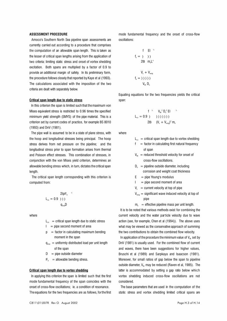
C811\01\007R Rev O August 2002 Page H.3 of H.14
ASSESSMENT PROCEDURE
Amoco's Southern North Sea pipeline span assessments are
currently carried out according to a procedure that comprises
the computation of an allowable span length. This is taken as
the lesser of critical span lengths arising from the application of
two criteria: limiting static stress and onset of vortex shedding
excitation. Both spans are multiplied by a factor of 0.9 to
provide an additional margin of safety. In its preliminary form,
the procedure follows closely that reported by Kaye et al (1993).
The calculations associated with the imposition of the two
criteria are dealt with separately below.
Critical span length due to static stress
In this criterion the span is limited such that the maximum von
Mises equivalent stress is restricted to 0.96 times the specified
minimum yield strength (SMYS) of the pipe material. This is a
criterion set by current codes of practice, for example BS 8010
(1993) and DnV (1981).
The pipe wall is assumed to be in a state of plane stress, with
the hoop and longitudinal stresses being principal. The hoop
stress derives from net pressure on the pipeline; and the
longitudinal stress prior to span formation arises from thermal
and Poisson effect stresses. This combination of stresses, in
conjunction with the von Mises yield criterion, determines an
allowable bending stress which, in turn, dictates the critical span
length.
The critical span length corresponding with this criterion is
computed from:
2IpFb ½ Lss = 0.9 )))
ó qmaxD û
where
Lss = critical span length due to static stressI = pipe second moment of area
p = factor in calculating maximum bending moment in the span
qmax = uniformly distributed load per unit length
of the spanD = pipe outside diameter
Fb = allowable bending stress.
Critical span length due to vortex shedding
In applying this criterion the span is limited such that the first
mode fundamental frequency of the span coincides with the
onset of cross-flow oscillations; ie. a condition of resonance.
The equations for the two frequencies are as follows, for the first
mode fundamental frequency and the onset of cross-flow
oscillations:
f EI ½
fs = ) )) 2B ó meL4û
Vc + Vwsig
fo = )))))
Vrth Do
Equating equations for the two frequencies yields the critical
span:
f ½ Vrth2 Do
2 EI ¼
Lcv = 0.9 ) )))))))
ó 2Bû ó (Vc + Vwsig)2 me û
where
Lcv = critical span length due to vortex sheddingf = factor in calculating first natural frequency
of spanVrth = reduced threshold velocity for onset of
cross-flow oscillations.
Do = pipeline outside diameter, including corrosion and weight coat thickness
E = pipe Young's modulusI = pipe second moment of area
Vc = current velocity at top of pipe
Vwsig = significant wave induced velocity at top of pipe
me = effective pipeline mass per unit length.
It is to be noted that various methods exist for combining the
current velocity and the water par t icle velocity due to wave
action (see, for example, Chen et al (1994)). The above uses
what may be viewed as the conservative approach of summing
the two contributions to obtain the combined flow velocity.
In application of the procedure the minimum value of Vrth set by
DnV (1981) is usually used. For the combined flow of current
and waves, there have been suggestions for higher values,
Bruschi et al (1989) and Sarpkaya and Isaacson (1981).
Moreover, for small ratios of gap below the span to pipeline
outside diameter, Vrth may be reduced (Raven et al, 1985). The
latter is accommodated by setting a gap ratio below which
vortex shedding induced cross-flow oscillations are not
considered.
The base parameters that are used in the computation of the
static stress and vortex shedding limited critical spans are

C811\01\007R Rev O August 2002 Page H.4 of H.14
summarised in Table 1. The axial restraint factor 8, i s a
parameter introduced for the purpose of assessing the
conservatism implicit in assuming full axial restraint at the ends
of the pipeline span. This assumption relates to the computation
of the longitudinal thermal and Poisson stresses in the pipeline.
The factor may only vary between zero (representing complete
axial freedom) and unity (representing complete axial fixity).
The parameters p and f appear independently in the equations
pertaining to static stress and vortex shedding. However, insofar
as they embody the effects of span end conditions and effective
axial force they are not totally independent variables. Moreover,
the effects of axial force on those parameters can be very
significant. Kaye et al (1993) have suggested a formula relating
f to effective axial force in the pipeline and span length. In
current practice, the choice of values assigned to p and f has
been influenced by field measurement data provided by Murray
(1992).
SENSITIVITY METHODOLOGY
The purpose of the work was to identify the conservatism in
Amoco's assessment procedure. Attention was focused,
however, on the data itself and its use within the assessment
method. In the work reported here no attempt was made to
appraise the relative conservatism between the method currently
used and others. The objectives were to gain insight into which
variables exerted the greatest (and the least) influence on limiting
spans, and to appraise the extent to which those with the
greatest influence contributed to the conservatism of the limiting
span magnitudes.
The sensitivity methodology chosen for the present requirement
is Monte Carlo simulation. This has the advantages of being
easy to understand conceptually, rapidly applied, and enabled
the required objectives to be met.
The technique used, therefore, corresponds with a Level Three
reliability method. It should be reemphasised, however, that
reliability analysis per se is not being performed. The approach
represents the application of a reliability technique to assess the
sensitivity of a deterministically-based assessment procedure, as
it is applied in practice. Its value is in helping to distinguish
those parameters which govern the assessment and for which
more accurate data might reduce the conservatism in cu rrent
assessments. A software package called "Crystal Ball" marketed
by Decisioneering was used to perform the calculations.
ANALYSES PERFORMED AND RESULTS
Three types of analyses were performed on two pipelines. The
pipelines are referred to in this paper as `A' and `B' and the
analyses were denoted as follows:
! deterministic
! primary sensitivity
! secondary sensitivity
In the deterministic analyses each of the chosen pipelines was
subjected to the assessment procedure as detailed earlier. Each
of the parameters listed in Table 1, however, took a single fixed
value as dictated by the normal requirements of the procedure.
The limiting span lengths due to static stress, vortex shedding
and the governing of the two were computed. The purpose of
obtaining these was to provide reference critical spans around
which observations concerning the span distributions (obtained
from the sensitivity analyses) could be based.
In primary sensitivity analyses, Monte Carlo simulations were
performed wherein each of the parameters listed in Table 1, was
assigned a frequency distribution. For the purposes of these
primary analyses it was felt that, where appropriate, distributions
should be set to as wide a spread as was reasonable. The aims
of the primary analyses were:
! To identify key parameters to which the
computation of limiting spans is most sensitive,
thereby highlighting parameters to be concentrated
upon in the secondary analyses.
! Equally importantly, the converse of the above.
! To determine, subject to the input distributions
used, the key statistics of the limiting span
distributions.
! To highlight within the distributions of critical span
the predominance of one of the governing criteria:
static stress or vortex shedding.
The reason for setting the parameter distributions to have a
wide spread was that, if a parameter turned out to be highly
ranked in sensitivity terms, the effect of its spread was to be
investigated in the secondary sensitivity analyses. Conversely, if
a parameter turned out to have a low sensitivity rating based on
a wide spread of data, then it could be reasonably dismissed
from further consideration.
In the secondary sensitivity analyses, Monte Carlo simulations
were again per formed, but adjustments were made to the
frequency distributions used in the primary analyses for
parameters identified as highly ranked. In broad terms, the
purpose of making these adjustments was to invest igate their
effect on sensitivity, distributions of limiting spans and governing
criterion.
Deterministic analyses
The magnitude of the input values used in the deterministic
analyses are summarised in Table 2. It is seen that the principal
differences between the two pipelines relate to:
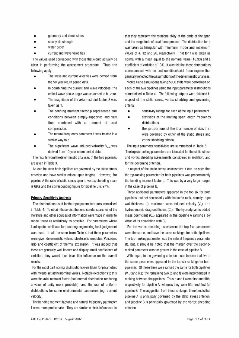
C811\01\007R Rev O August 2002 Page H.5 of H.14
! geometry and dimensions
! steel yield strength
! water depth
! current and wave velocities
The values used correspond with those that would actually be
taken in performing the assessment procedure. Thus the
following apply:
! The wave and current velocities were derived from
the 50 year return period data.
! In combining the current and wave velocities, the
critical wave phase angle was assumed to be zero.
! The magnitude of the axial restraint factor 8 was
taken as 1.
! The bending moment factor p represented end
conditions between simply-supported and fully
fixed combined with an amount of axial
compression.
! The natural frequency parameter f was treated in a
similar way to p.
! The significant wave induced velocity Vwsig was
derived from 10 year return period data.
The results from the deterministic analyses of the two pipelines
are given in Table 3.
As can be seen both pipelines are governed by the static stress
criterion and have similar critical span lengths. However, for
pipeline A the ratio of static stress span to vortex shedding span
is 69% and the corresponding figure for pipeline B is 97%.
Primary Sensitivity Analysis
The distributions used for the input parameters are summarised
in Table 4. To obtain these distributions careful searches of the
literature and other sources of information were made in order to
model these as realistically as possible. For parameters where
inadequate detail was forthcoming engineering best-judgement
was used. It will be seen from Table 4 that three parameters
were given deterministic values: steel elastic modulus, Poisson's
ratio and coefficient of thermal expansion. It was judged that
these are generally well known and display small coefficients of
variation; they would thus bear little influence on the overall
results.
For the most part normal distributions were taken for parameters
with means set at the nominal values. Notable exceptions to this
were the axial restraint factor (half-normal distribution rendering
a value of unity more probable), and the use of uniform
distributions for some environmental parameters (eg. current
velocity).
The bending moment factor p and natural frequency parameter
f were more problematic. They are similar in their influences in
that they represent the rotational fixity at the ends of the span
and the magnitude of axial force present. The distribution for p
was taken as triangular with minimum, mode and maximum
values of 4, 12 and 20, respectively. That for f was taken as
normal with a mean equal to the nominal value (16.33) and a
coefficient of variation of 13%. It was felt that these distributions
corresponded with an end condition/axial force regime that
generally reflected the assumptions of the deterministic analyses.
Monte Carlo simulations taking 5000 trials were performed on
each of the two pipelines using the input parameter distributions
summarised in Table 4. The following outputs were obtained in
respect of the static stress, vortex shedding and governing
criteria:
! sensitivity ratings for each of the input parameters
! statistics of the limiting span length frequency
distributions
! the proportions of the total number of trials that
were governed by either of the static stress and
vortex shedding criteria.
The input parameter sensitivities are summarised in Table 5.
The top six ranking parameters are tabulated for the static stress
and vortex shedding assessments considered in isolation, and
for the governing criterion.
In respect of the static stress assessment it can be seen that
the top-ranking parameter for both pipelines was predominantly
the bending moment factor p. This was by a very large margin
in the case of pipeline B.
Three additional parameters appeared in the top six for both
pipelines, but not necessarily with the same rank, namely: pipe
wall thickness (t); maximum wave induced velocity (Vw) and
hydrodynamic drag coefficient (Cd). The hydrodynamic added
mass coefficient (Cm) appeared in the pipeline A rankings by
virtue of its correlation with Cd.
For the vortex shedding assessment the top five parameters
were the same, and have the same rankings, for both pipelines.
The top-ranking parameter was the natural frequency parameter
(f), but, it should be noted that the margin over the second-
ranked parameter was far greater in the case of pipeline B.
With regard to the governing criterion it can be seen that five of
the same parameters appeared in the top six rankings for both
pipelines. Of these three were ranked the same for both pipelines
(Vc, t and Cd); the remaining two (p and f) were interchanged in
ranking between the pipelines. Thus p and f were first and fifth,
respectively for pipeline A, whereas they were fifth and first for
pipeline B. The suggestion from these rankings, therefore, is that
pipeline A is principally governed by the static stress criterion,
and pipeline B is principally governed by the vortex shedding
criterion.

C811\01\007R Rev O August 2002 Page H.6 of H.14
The statistics of the limiting span length frequency distributions
are summarised in Table 6. Information is given on mean and
coefficient of variation, as well as the span lengths
corresponding with the 2.5%, 5.0% and 50% percentiles.
The mean span lengths tended to reflect the dominance of one
or other of the static stress or vortex shedding criteria. Pipeline
A had a lower mean for static stress than for vortex shedding
with the governing mean closer in value to that of the static
stress. The converse of this was true for pipeline B. For both
pipeline cases the coefficient of variation for static stress
exceeded that for vortex shedding, and it is noticeable that for
pipeline B the coefficients of variation for vortex shedding and
that corresponding with the governing criterion were very close
in value.
The pattern exhibited by the percentile values for the governing
limiting span distributions tended to follow the dominant
criterion. Thus governing percentiles were close in value to
static stress criterion ones for pipeline A, whereas they were
close in value to vortex shedding criterion ones for pipeline B. In
comparing the deterministically computed governing span
lengths with the corresponding percentile values it is seen that
for pipeline A the deterministic value lies between the 2.5% and
5.0% percentile values, whereas for pipeline B the deterministic
value exceeds the 5.0% percentile value.
Finally the dominance of a particular criterion for each pipeline
was confirmed by the percentage of trials results. Of these
pipeline B is the most significant in that 90% of the trials were
governed by the vortex shedding criterion; this is in contrast with
the simple deterministic calculations performed earlier which
determined pipeline B to be governed by the static stress
criterion.
Secondary Sensitivity Analyses
It is evident from the primary sensitivity analyses that the
principal parameters that affected limiting span distributions the
most and, therefore, were investigated further in the secondary
analyses were as follows:
! bending moment factor p
! natural frequency parameter f
! pipe wall thickness t
! current velocity Vc
! maximum wave induced velocity Vw
! significant wave induced velocity Vwsig
The additional distributions used for these parameters are
summarised in Table 7. This table reiterates the fact that some
parameters (t a n d Vc) are common to both limiting span
calculations whereas others are unique to one or other. Hence,
changes to individual input parameter distributions were
assessed in the following way: p and Vw on A only; f and Vwsig on
B only; and t and Vc on both A and B.
The principal reasons for making the changes to the
distributions were to observe the effects of changing mean,
mode, COV and distribution of the key input parameters. In the
secondary analysis the distributions relevant to each pipeline
were changed individually; thus seven analyses were carried out
for pipeline A, and 6 analyses for pipeline B.
The following results were observed for the parameters t, V c, Vw,
Vwsig:
t A significant reduction in the COV of the pipe wall
thickness distribution had the effect, for both
pipelines, of removing t from the top six ranking
parameters. The reduction had a negligible effect
on the variability of the critical span length and the
governing criteria.
Vc The change in distribution tended to give a slightly
increased ranking percentage, but had little effect
on the critical span statistics or governing criteria for
both pipelines.
Vw Increasing the COV of the distribution had the
effects of: promoting the parameter up the
sensitivity rankings to the extent that with a COV of
20% Vw became the second ranked parameter after
p; increasing the COV of the critical span
distributions, thereby decreasing the percentiles.
The effects on the ruling criterion were negligible.
Vwsig The results regarding this parameter were very
similar to those for Vw except that the changes were
less pronounced and less significant.
Of most significance were the results pertaining to changes
made in the bending moment factor p and the natural frequency
parameter f, in relation to pipelines A and B, respectively.
Table 8 summarises the effects of p on the top six ranking
input parameters corresponding with the governing criterion for
pipeline A. For the three triangular distributions it is seen that the
effect of reducing the mode value was to increase the sensitivity
to p; this occurs with an associated decrease in the rankings of
the other parameters. Similar effects were observed in changing
from the triangular to the normal distribution with the same
mean; the result was, for example, to equalise the rankings of p
and Vc.
The statistics of the limiting span length frequency distribution
are given in Table 9. For the triangular distributions it may be
observed that the reduction in the mode value of p from 16 to 8
had the effect of reducing the mean value, and each of the three
percentile values, but increasing the COV. These effects are due
to the general increase in the possibility of smaller spans.

C811\01\007R Rev O August 2002 Page H.7 of H.14
However, in contrast, the skewness increased (became less
negative) as the mode value decreased; thus, higher values of
mode value led to a longer tail over the smaller governing limiting
span length than lower values. In comparing the triangular with
the normal distribution it can be seen that the only significant
changes were a decrease in the coefficient of variation, and
increases in the percentiles.
Regarding the proportions of trials dictated by the two criteria,
the effect of reducing the mode value in the triangular
distributions was to increase the proportion pertaining to the
static stress. It is notable that for a mode value of 16 the
proportion of trials that were governed by vortex shedding was
a half.
For pipeline B the corresponding results for changes in the
distribution for f are given in Tables 10 and 11 for top ranking
parameters and limiting span length statistics, respectively.
In Table 10 it is seen that a decrease in the COV of f from 13%
to 2% (whilst maintaining the mean value) drastically reduced the
sensitivity to f, thereby rendering Vc the top-ranking parameter by
a very large margin. An increase in the mean from 16.3 to 25.1,
resulted in p and Vc becoming the first and second ranked
parameters, respectively, with f fairly insignificant.
Table 11 shows that a decrease in the COV of f from 13% to
2% generally led to increases in the 2.5% and 5% percentiles, but
most significant were the changes in the skewness of the
limiting span distributions: of the order of twenty times. This
indicates that the COV changes resulted in the development of
a significant tail in the limiting span distribution at the lower end.
In changing the mean of f from 16.3 to 25.1 a doubling of the
skewness resulted, but little change in the percentile values
occurred. This is surprising given the significant alteration made,
but can be explained by the fact that in making the change the
pipeline became less dominated by vortex shedding. This is
evidenced by the dramatic increase in sensitivity to p (Table 10)
and the large increase in the proportion of trials governed by
static stress (Table 11).
DISCUSSION
The primary sensitivity analyses revealed that of the 26 input
parameters 6 exerted the greatest influence on critical spans.
However, pipe wall thickness t was effectively removed from
amongst the top six rankings when it was given a more realistic
distribution in secondary analyses. The remaining 5 could be
classified into two groups pertaining to: modelling of the span
response, and hydrodynamic loading. Into the first group fell:
! bending moment factor p
! natural frequency parameter f
and these are, in turn, functions of span end support conditions
and effective axial force in the pipe, not explicitly admitted to the
assessment methods.
Into the second group fell:
! current velocity Vc
! maximum wave induced velocity Vw
! significant wave induced velocity Vwsig
It was found in the primary analyses that of these two groups
the parameters falling into the first were by far the more
influential. In considering the second group the current velocity
Vc tended to exert the most influence. Of the two pipelines
considered, pipeline A was deemed dominated by the static
stress criterion and pipeline B by the vortex shedding criterion.
These observations tended to be reflected in some of the
secondary sensitivity analyses, wherein changes were made to
the distributions of the key parameters on an individual basis.
Alterations made to the distributions of Vw and Vwsig in terms of
variation of the COV values tended only to result in alteration to
their ranking, and had marginal effects on critical span
distribution and governing criterion majority. Of the two, the
effects of Vw were the more pronounced. The change made to
Vc (which was different to the changes made to the distributions
of the other two parameters in its group) tended to strengthen its
ranking in the top six parameters, with marginal effects on the
critical span distribution and majority criterion.
The changes made to the distributions of p and f tended to
produce the most significant effects. The results also illustrated
the interaction between the two criteria in contributing to the
governing limiting span.
Thus, in the case of pipeline A (which from the primary
analyses was deemed to be static stress dominated) changes in
the mode value and type for the distribution used for p could
reduce its influence and increase the ranking of Vc and, to a
lesser extent, f. With increases in the mode value the balance
between trials governed by static stress or vortex shedding could
be radically altered to the extent of half the trials becoming
governed by either criterion.
In a similar manner, for pipeline B (which was deemed to be
vortex shedding dominated by the primary analyses) a reduction
in the COV of the distribution for f (the most important as far as
the vortex shedding criterion is concerned) could make its
ranking of this parameter quite low and promote Vc to the highest
ranked. A simultaneous change in the mean and the COV had
the effect of making p and Vc the top two ranking parameters
respectively and greatly increased the number of trials governed
by the static stress criterion.
Most important for pipeline B, was that, having established the
significance of f from the primary analyses, favourable
improvements made to the distribution for f did not produce
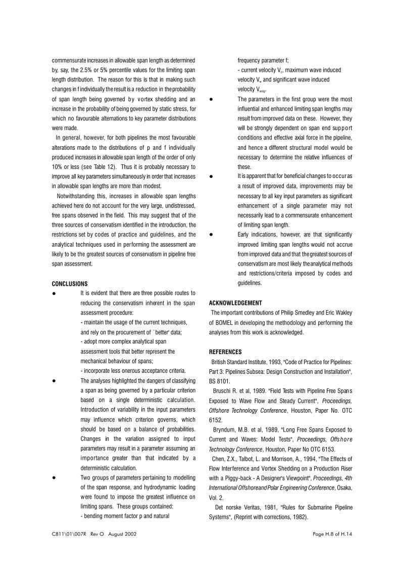
C811\01\007R Rev O August 2002 Page H.8 of H.14
commensurate increases in allowable span length as determined
by, say, the 2.5% or 5% percentile values for the limiting span
length distribution. The reason for this is that in making such
changes in f individually the result is a reduction in the probability
of span length being governed by vortex shedding and an
increase in the probability of being governed by static stress, for
which no favourable alternations to key parameter distributions
were made.
In general, however, for both pipelines the most favourable
alterations made to the distributions of p and f individually
produced increases in allowable span length of the order of only
10% or less (see Table 12). Thus it is probably necessary to
improve all key parameters simultaneously in order that increases
in allowable span lengths are more than modest.
Notwithstanding this, increases in allowable span lengths
achieved here do not account for the very large, undistressed,
free spans observed in the field. This may suggest that of the
three sources of conservatism identified in the introduction, the
restrictions set by codes of practice and guidelines, and the
analytical techniques used in per forming the assessment are
likely to be the greatest sources of conservatism in pipeline free
span assessment.
CONCLUSIONS
! It is evident that there are three possible routes to
reducing the conservatism inherent in the span
assessment procedure:
- maintain the usage of the current techniques,
and rely on the procurement of `better' data;- adopt more complex analytical span
assessment tools that better represent the
mechanical behaviour of spans;
- incorporate less onerous acceptance criteria.
! The analyses highlighted the dangers of classifying
a span as being governed by a particular criterion
based on a single deterministic calculation.
Introduction of variability in the input parameters
may influence which criterion governs, which
should be based on a balance of probabilities.
Changes in the variation assigned to input
parameters may result in a parameter assuming an
importance greater than that indicated by a
deterministic calculation.
! Two groups of parameters pertaining to modelling
of the span response, and hydrodynamic loading
were found to impose the greatest influence on
limiting spans. These groups contained:
- bending moment factor p and natural
frequency parameter f;
- current velocity Vc, maximum wave induced
velocity Vw and significant wave induced
velocity Vwsig.
! The parameters in the first group were the most
influential and enhanced limiting span lengths may
result from improved data on these. However, they
will be strongly dependent on span end support
conditions and effective axial force in the pipeline,
and hence a different structural model would be
necessary to determine the relative influences of
these.
! It is apparent that for beneficial changes to occur as
a result of improved data, improvements may be
necessary to all key input parameters as significant
enhancement of a single parameter may not
necessarily lead to a commensurate enhancement
of limiting span length.
! Early indications, however, are that significantly
improved limiting span lengths would not accrue
from improved data and that the greatest sources of
conservatism are most likely the analytical methods
and restrictions/criteria imposed by codes and
guidelines.
ACKNOWLEDGEMENT
The important contributions of Philip Smedley and Eric Wakley
of BOMEL in developing the methodology and performing the
analyses from this work is acknowledged.
REFERENCES
British Standard Institute, 1993, "Code of Practice for Pipelines:
Part 3: Pipelines Subsea: Design Construction and Installation",
BS 8101.
Bruschi R. et al, 1989. "Field Tests with Pipeline Free Spans
Exposed to Wave Flow and Steady Current", Proceedings,
Offshore Technology Conference, Houston, Paper No. OTC
6152.
Bryndum, M.B. et al, 1989, "Long Free Spans Exposed to
Current and Waves: Model Tests", Proceedings, Offshore
Technology Conference, Houston, Paper No OTC 6153.
Chen, Z.X., Talbot, L. and Morrison, A., 1994, "The Effects of
Flow Interference and Vortex Shedding on a Production Riser
with a Piggy-back - A Designer's Viewpoint", Proceedings, 4th
International Offshore and Polar Engineering Conference, Osaka,
Vol. 2.
Det norske Veritas, 1981, "Rules for Submarine Pipeline
Systems", (Reprint with corrections, 1982).

C811\01\007R Rev O August 2002 Page H.9 of H.14
Health and Safety Executive, 1993, "Structural Analysis of
Pipeline Spans", OTI 93 613, HMSO, London.
Irvine, M., 1993, "On the Mechanics of Spanning in Submarine
Pipelines", Proceedings, 3rd International Offshore and Polar
Engineering Conference, Singapore, Vol. 2, pp.98-105.
Kaye, D et al, 1993, "Pipeline Freespan Evaluation: A New
Methodology", Proceedings, Offshore Europe Conference,
Aberdeen, Paper No SPE 26774.
Murray, B G., 1992, "Pipeline Freespan Vibration Monitoring",
Development Engineering International Limited, Report Nos
PTIPUB/P3 and PS047/01.
Orgill, G et al, 1992, "Current Practice in Determining Allowable
Pipeline Free Spans", Proceedings, 11th Offshore Mechanics and
Arctic Engineering Conference, Vol. 2-A, pp.139-145.
Raven, P.W.J et al, 1985, "Full-scale Dynamical Testing of
Submarine Pipeline Spans", Proceedings, Offshore Technology
Conference, Houston, Paper No. OTC 5005.
Reid, D.L., 1990, "A Generalised in-Line Vortex-Induced
Vibration Assessment Method", Proceedings, Offshore
Technology Conference, Houston, Paper No OTC 6365.
Sarpkaya, T. and Isaacson, M, 1981, "Mechanics of Wave
Forces for Offshore Structures", van Nostrand Reinhold Co., New
York.
Sheppard, D.M. and Omar, A.F., 1992, "Vortex-induced
Loading on Offshore Structures: A Selective Review of
Experimental Work", Proceedings, Offshore Technology
Conference, Houston, Paper No OTC 6817.
Skomedal, E., 1991, "Static Calculation of Pipeline Free Spans",
Proceedings, 1st International Offshore and Polar Engineering
Conference, Edinburgh, Vol. 2, pp.281-289. Tassini, P.A., et al,
1989, "The Submarine Vortex Shedding Project: Background,
Overview and Future Fall Out on Pipeline Design", Proceedings,
Offshore Technology Conference, Houston, Paper No OTC
6157.
Tura, F., et al, 1994a, "Guidelines for Free Spanning Pipelines:
Outstanding Items and Technological Innovations", ASPECT-94,
Society for Underwater Technology, Vol. 33, pp.59-76.
Tura, F., et al, 1994b, "Guidelines for Free Spanning Pipelines:
the GUDESP Project", Proceedings, 13th Offshore Mechanics
and Arctic Engineering Conference, Vol V, pp.247-256.
TABLE 1 LIST OF PARAMETERS USED IN SPAN ASSESSMENT
Input parameterUsed in
Staticstress
Vor texshedding
Pipe outside diameter D T T
Pipe wall thickness t T TCorrosion coat thickness te T T
Weight coat thickness tc T T
Steel density Ds T T
Corrosion coat density De T T
Weight coat density Dc T T
Steel elastic modulus E T T
Steel Poisson's ratio < T X
Steel SMYS Fy T X
Steel thermal expansion coeff. " T X
Axial restraint factor ( T X
Bending moment factor p T X
Natural frequency parameter f X T
Max. int. operating pressure pi T X
Contents density Di T T
Contents temperature 2i T X
Min. water depth at LAT h T X
Current speed: top of pipe Vc T T
Max. wave induced velocity Vw T X
Signif. wave induced velocity Vwsig T T
Reduced threshold velocity Vrth X T
Local seawater density Dw T X
Local seawater temperature 2a T X
Hydrodynamic drag coeff. Cd T X
Hydrodynamic added mass coeff Cm X T

C811\01\007R Rev O August 2002 Page H.10 of H.14
TABLE 2 MAGNITUDES OF PARAMETERS USED IN DETERMINISTIC ANALYSES
Input parameterPipeline
A B Units
Pipe outside diameter D 762 273 mm
Pipe wall thickness t 17.5 11.1 mm
Corrosion coat thickness te 5.6 5.0 mm
Weight coat thickness tc 33 45 mm
Steel density Ds 7850 7850 kg/m3
Corrosion coat density De 1200 1438 kg/m3
Weight coat density Dc 3124 2243 kg/m3
Steel elastic modulus E 207 207 GPa
Steel Poisson's ratio < 0.3 0.3 -
Steel SMYS Fy 358 413 MPa
Steel thermal expansion coeff. " 0.0000116 0.0000116 /°C
Axial restraint factor 8 1.0 1.0 -
Bending moment factor p 8.0 8.0 -
Natural frequency parameter f 16.33 16.33 -
Max internal operating pressure pi 9.0 13.9 MPa
Contents density Di 585 806 kg/m3
Contents temperature 2i 49 49 °C
Min. water depth at LAT h 29.5 141.0 m
Current speed: top of pipe Vc 1.07 0.54 m/s
Max. wave induced velocity Vw 3.22 1.28 m/s
Signif. wave induced velocity Vwsig 1.1 0.29 m/s
Reduced threshold velocity Vrth 3.5 3.5 m/s
Local seawater density Dw 1025 1025 kg/m3
Local seawater temperature 2a 6 4 °C
Hydrodynamic drag coeff. Cd 1.05 1.05 -
Hydrodynamic added mass coeff. Cm 1.0 1.0 -
TABLE 3 LIMITING SPANS FROM DETERMINISTIC ANALYSES
CriterionLimiting span (m) for pipeline
A B
Static stress
Vor tex shedding
Critical
29.8
42.9
29.8
26.3
27.0
26.3
Static: Vor tex span ratio 69% 97%

C811\01\007R Rev O August 2002 Page H.11 of H.14
TABLE 4 FREQUENCY DISTRIBUTIONS FOR INPUT PARAMETERS USED IN PRIMARY SENSITIVITY ANALYSES
Input parameterUsed in
Distribution usedStaticstress
Vor texshedding
Pipe outside diameter D T T Normal: Mean = Nominal, COV = 1.5%
Pipe wall thickness t T T Normal: Mean = Nominal, COV = 10%
Corrosion coat thickness te T T Normal: Mean = Nominal, COV = 7%
Weight coat thickness tc T T Normal: Mean = Nominal, COV = 10%
Steel density Ds T T Normal: Mean = 7850, COV = 0.5%
Corrosion coat density De T T Normal: Mean = Nominal, COV = 1%
Weight coat density Dc T T Normal: Mean = Nominal, COV = 5%
Steel elastic modulus E T T Deterministic value
Steel Poisson's ratio < T X Deterministic value
Steel SMYS Fy T X Normal: Mean = calculated COV = 5%
Steel thermal exp. coeff. " T X Deterministic value
Axial restraint factor ( T X Half-normal: Mean 1.0, COV = 33%
Bending moment factor p T X Triangular: Min=4, mode=12, max=20
Natural frequency parameter f X T Normal: Mean = 16.33, COV = 13%
Max. int. operating pressure pi T X Normal: Mean = Nominal, COV = 10%
Contents density Di T T Normal: Mean = Nominal, COV = 3%
Contents temperature 2i T X Normal: Mean = Nominal, COV = 6%
Min. water depth at LAT h T X Normal: Mean = Nominal, COV = 2%
Current speed: top of pipe Vc T T Uniform: Min, Max from data
Max. wave induced velocity Vw T X Normal: Mean = Nominal, COV = 10%
Signif. wave induced velocity Vwsig T T Normal: Mean = Nominal, COV = 10%
Reduced threshold velocity Vrth X T Uniform: Min = 3.5, Max = 3.8
Local seawater density Dw T X Normal: Mean = Nominal, COV = 0.5%
Local seawater temperature 2a T X Triangular: Min=0, mode=6, Max=9°C
Hydrodynamic drag coeff. Cd T X Normal: Mean = Nominal, COV = 15%
Hydrodynamic added mass coeff Cm X T Normal: Mean = Nominal, COV = 15%
TABLE 5 TOP SIX RANKING INPUT PARAMETERS MEASURED BY
CONTRIBUTION TO VARIANCE, FROM THE PRIMARY SENSITIVITY ANALYSES
Pipeline A Pipeline B
Static Vor tex Governing Static Vor tex Governing
% % % % % %
p 47.0 f 44.9 p 40.2 p 76.1 f 64.9 f 61.0
Vw 10.9 Vc 34.3 Vc 14.7 tc 7.3 Vc 16.0 Vc 15.1
t 10.7 Vwsig 8.6 t 13.0 t 4.7 Vwsig 5.5 t 6.8
Cd 10.3 t 4.5 Vw 8.9 Fy 4.6 t 4.7 Vwsig 5.4
Cm 6.0 Cm 2.3 f 6.2 Vw 1.5 Cm 3.1 p 3.8
Vc 5.8 Vrth 2.1 Cd 5.5 Cd 1.3 Cd 2.2 Cd 1.5
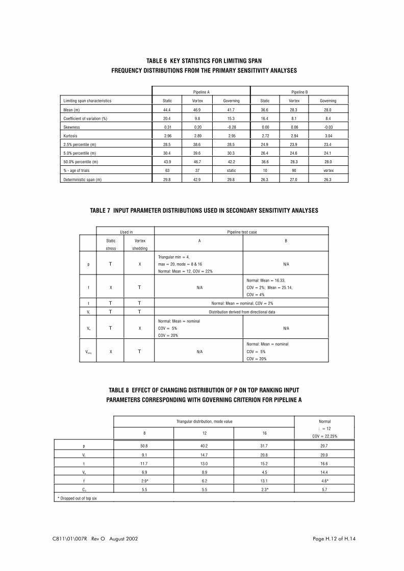
C811\01\007R Rev O August 2002 Page H.12 of H.14
TABLE 6 KEY STATISTICS FOR LIMITING SPAN
FREQUENCY DISTRIBUTIONS FROM THE PRIMARY SENSITIVITY ANALYSES
Pipeline A Pipeline B
Limiting span characteristics Static Vor tex Governing Static Vor tex Governing
Mean (m) 44.4 46.9 41.7 36.6 28.3 28.0
Coefficient of variation (%) 20.4 9.8 15.3 16.4 8.1 8.4
Skewness 0.31 0.20 -0.28 0.00 0.06 -0.03
Kurtosis 2.96 2.89 2.95 2.72 2.94 3.04
2.5% percentile (m) 28.5 38.6 28.5 24.9 23.9 23.4
5.0% percentile (m) 30.4 39.6 30.3 26.4 24.6 24.1
50.0% percentile (m) 43.9 46.7 42.2 36.6 28.3 28.0
% - age of trials 63 37 static 10 90 vor tex
Deterministic span (m) 29.8 42.9 29.8 26.3 27.0 26.3
TABLE 7 INPUT PARAMETER DISTRIBUTIONS USED IN SECONDARY SENSITIVITY ANALYSES
Used in Pipeline test case
Static
stress
Vor tex
shedding
A B
p T X
Triangular min = 4,
max = 20, mode = 8 & 16
Normal: Mean = 12, COV = 22%
N/A
f X T N/A
Normal: Mean = 16.33,
COV = 2%; Mean = 25.14,
COV = 4%
t T T Normal: Mean = nominal, COV = 2%
Vc T T Distribution derived from directional data
Vw T X
Normal: Mean = nominal
COV = 5%
COV = 20%
N/A
Vwsig X T N/A
Normal: Mean = nominal
COV = 5%
COV = 20%
TABLE 8 EFFECT OF CHANGING DISTRIBUTION OF P ON TOP RANKING INPUT
PARAMETERS CORRESPONDING WITH GOVERNING CRITERION FOR PIPELINE A
Triangular distribution, mode value Normal
: = 12
COV = 22.25%8 12 16
p 50.8 40.2 31.7 20.7
Vc 9.1 14.7 20.8 20.0
t 11.7 13.0 15.2 16.6
Vw 6.9 8.9 4.5 14.4
f 2.9* 6.2 13.1 4.6*
CD 5.5 5.5 2.3* 5.7
* Dropped out of top six

C811\01\007R Rev O August 2002 Page H.13 of H.14
TABLE 9 EFFECT OF CHANGING DISTRIBUTION OF P
ON GOVERNING LIMITING SPAN DISTRIBUTION KEY STATISTICS FOR PIPELINE A
Triangular distribution, mode value Normal
: = 12
COV = 22.25%Limiting span statistic 8 12 16
Mean (m) 39.9 41.7 43.0 41.8
Coefficient of variation (%) 17.2 15.3 14.5 14.2
Skewness -0.11 -0.28 -0.35 -0.33
Kurtosis 2.73 2.95 3.31 3.21
2.5% percentile (m) 26.5 28.5 29.5 29.3
5.0% percentile (m) 28.1 30.3 31.8 31.7
50% percentile (m) 40.2 42.2 43.4 42.0
Static stress (%) 73 63 50 62
Vor tex shedding (%) 27 37 50 38
TABLE 10 EFFECT OF CHANGING DISTRIBUTION OF F ON TOP RANKING INPUT
PARAMETERS CORRESPONDING WITH GOVERNING LIMITING CRITERION FOR PIPELINE B
Normal distribution for f
Mean 16.33 16.32 25.14
COV (%) 13.0 2.0 3.8
f 61.0 3.0 4.3
Vc 15.1 59.5 23.0
t 6.8 0.7* 0.0*
Vwsig 5.4 14.8 5.5
p 3.8 3.6 51.9
Cd 1.5 1.4* 0.1*
* Dropped out of top six
TABLE 11 EFFECT OF CHANGING DISTRIBUTION OF F ON GOVERNING LIMITING
SPAN DISTRIBUTION KEY STATISTICS FOR PIPELINE B
Normal distribution for f
Mean 16.33 16.32 25.14
COV (%) 13.0 2.0 3.8
Mean (m) 28.0 28.2 33.5
Coefficient of variation (%) 8.4 5.1 9.2
Skewness -0.03 -0.66 -1.26
Kurtosis 3.04 5.01 4.75
2.5% percentile (m) 23.4 25.2 25.5
5.0% percentile (m) 24.1 26.0 27.0
50% percentile (m) 28.0 28.2 34.2
Static stress (%) 10 8 39
Vor tex shedding (%) 90 92 61

C811\01\007R Rev O August 2002 Page H.14 of H.14
TABLE 12 COMPARISON BETWEEN DETERMINISTIC, PRIMARY AND SECONDARY ANALYSES RESULTS
Pipeline A Pipeline B
Primary Secondary
p only
Primary Secondary
f only
Table 6 Table 9 Table 6 Table 11
Mean (m) 41.7 41.8 28.0 33.5
Coefficient of variation (%) 15.3 14.2 8.4 9.2
2.5% percentile (m) 28.5 29.3 23.4 25.5
5.0% percentile (m) 30.3 31.7 24.1 27.0
Deterministic (m)* 29.8 29.8 26.3 26.3
* Results from Table 3