Alex Thomas12 March 2010Professor William SteinMath 414Twelve Steps:The Proofs for the Prime Number Theorem and Prime Number Theorem in Arithmetic Progression by Newman(via Zagier) and Soprounov Respectively

In this project I will explain the proof of the Prime Number Theorem(PNT) by D.J. Newman, as described by D. Zagier, and the proof by Ivan Soprounov of prove the Prime Number Theorem in Arithmetic Progression(PNTAP). Once I have explained the asymptotic estimates of the prime counting function, and the prime counting function for primes congruent to some number modulo another, I will test the latter estimate by means of a program I have written in Sage.We will begin with Newman’s proof for the PNT

Newman’s proof of the PNT begins with establishing Euler’s product formula. First, let us show the Riemann zeta function. This function was first examined by Euler in a proof of Euclid’s theorem, as well as by Dirichlet, but Riemann was the first to study in-depth as a function of a complex variable1, hence its name.Definition 1: the Riemann zeta functionζ ( s)≝∑

n=1

∞ 1ns, s∈C

Let us now examine the expanded series.Eq. 1ζ ( s)=∑

n=1

∞ 1ns

=1+ 12s

+ 13s

+ 14s

+ 15s

+…

Now we multiply both sides by the second term.Eq. 212sζ ( s )= 1

2s∑n=1

∞ 1ns

= 12s

+ 14s

+ 16s

+ 18s

+ 110s

+…

Next we subtract Eq. 2 from Eq, 1.1 LeVeque, 154, 155

Eq. 3ζ ( s )− 1

2sζ (s )=(1− 12s )ζ ( s )=1+ 1

3s+ 15s

+ 17s

+ 19s

+…

Then let us multiply both sides by the second term again. Eq. 413s (1− 1

2s )ζ ( s )= 13 s

+ 19s

+ 115s

+ 121 s

+ 127s

+…

As before, let us subtract Eq. 4 from Eq. 3.Eq. 5

(1− 13s )(1− 12s )ζ ( s)=1+ 1

5s+ 17s

+ 111s

+ 113s

+ 117s

+…

We do these same steps to obtain another factor.Eq. 6(1− 15 s )(1− 1

3 s )(1− 12s )ζ ( s )=1+ 1

7 s+ 111s

+ 113s

+ 117 s

+ 119s

+…

If we continue in this way the right-hand side approaches 1, and this gives us Eq. 7 ζ ( s)∏

p(1−p− s )=1

One can notice the similarity of this proof to the Sieve of Eratosthenes.Now solving for ζ ( s), we get the Euler product formula as desired.Result 1: Euler’s product formula

ζ ( s)=(∏p (1−p−s ))−1

=∏p

(1−p−s )−1

Next we will show that ζ ( s )− 1s−1 is analytic (Zagier uses the word ‘holomorphic’, which means the same in this situation)2 on {s∈C :R (s )>0 }, the right half of the complex plane.

We will transform the expression into something that will let us talk of analyticity. We can treat 1s−1 as the result of an improper integral, and then finesse the summand in the Riemann zeta function underneath the integral. The way this is done becomes obvious if you transform the rightmost side into the middle one.

2 Zagier, 1

Eq. 8ζ ( s)− 1

s−1=∑

n=1

∞ 1ns

−∫1

∞ 1x s dx=∑

n=1

∞

∫n

n+1 1ns

− 1xsdx

Now we examine the absolute value of the summed integral, whence we obtain Result 2: ζ ( s )− 1s−1 is analytic on {s∈C :R (s )>0 }

|∫1∞ 1ns

− 1xsdx|=|s∫1

∞

∫n

x 1us+1 dudx|≤ max

n≤u≤n+1| sus+1|= |s|

nR (s )+1

This shows that the summand is less than that of a convergent power series times a constant, ¿ s∨¿, so by the comparison test, it too must be convergent.Now we will show ∑

p≤ xlog (p )=O(x ), where O(x ) is big O notation, but first let us officially define this series as a function.Definition 2:θ(x )θ ( x )≝∑

p≤ xlog ( p )

First, we will try and get a handle on how fast θ(x ) changes with respect to x. Eq. 922n=(1+1 )2n=∑

i=0

n

(2ni )≥(2nn )≥ ∏n< p≤2n

p=eθ ( 2n )−θ (n )

This has given us something which we can manipulate by taking the log of both sides. Eq. 102n log (2 )≥θ (2n )−θ (n )

This gives us something with θ(x ) on the left side, and something O(x ) on the right. Eq. 11θ ( x )−θ( x2 )≤Cx ,C>log 2

Now we will sum these differences for over increasing powers of 2.Eq. 12∑i=0

∞

(θ( x2i )−θ( x2i+1 ))≤C∑

i=0

∞ x2i

Applying term by term cancellation on the left side, and the normal properties for a geometric series on the right, we obtainEq. 13θ ( x )≤C∑

i=0

∞ x2i

=2Cx

From this we see that Result 3θ(x )=O(x )

Now we will examine Φ ( s). Definition 3: Φ ( s )

Φ ( s)≝∑p

log (p )ps

We want to show that the Riemann zeta function has no zeroes for{s∈C :R ( s )≥1 }, also we will show that Φ ( s )− 1

s−1 is analytic there as well.To examine ζ ( s) for zeroes, we will look at the logarithmic derivative.

Eq. 14ddslog (ζ (s ) )=−d

dslog (∏p (1− p− s ))

The rules of logarithms lead us to use the product form of ζ ( s); these rules will allow us transform the logarithm of a product into a sum of logarithms.Eq. 15−ζ ' (s )ζ ( s)

=−ddslog (∏p (1−p−s )−1)=−d

ds ∑plog ( (1−p−s )−1 )=¿

−∑p

p−s log (p )

(1−p− s )2

(1−p−s )−1=∑

p

log ( p )ps−1

This leaves us with a suggestive form (the negative was appended to the logarithmic derivative in order to get us here), which we can manipulate to achieve our intended result. Eq. 16∑p

log ( p )p s−1

=∑p

log ( p )ps−1

−log (p )ps

+¿log (p )ps

=Φ (s )+∑p

log ( p )ps (ps−1 )

¿

Now, if we establish analyticity for the rightmost part, we will have completed both of our tasks. So now let us show that the series ∑p

log ( p )ps ( ps−1 ) is convergent by the comparison test.Eq. 17

| log ( p )ps ( ps−1 )|= log ( p )

pR ( s)|( ps−1 )|

Now we must get a handle on|( ps−1 )|, so let us separate off some of the series. Eq. 18∑p

log (p )ps ( ps−1 )

=∑p=2

n log ( p )ps ( ps−1 )

+∑p>n

log ( p )ps ( ps−1 )

The term on the right of the plus sign is finite, so let us work on the one on the left, but we will consider the value of p first.Eq. 19p>n⇒ pR ( s)>nR ( s) , p

R (s )

nR (s ) >1 ,R ( s )>0

This will eventually give us a finite number with which to work.3Eq. 20pR (s )− pR ( s )

nR (s ) =pR ( s)(1− 1nR ( s) )< pR ( s)−1

1

pR ( s )(1− 1nR ( s ) )

=K> 1pR ( s)−1

This gives us something to replace the troublesome |( ps−1 )|.Eq. 21log (p )

pR ( s )|( ps−1 )|< log (p )K p2 R (s )

Which is convergent for2 R (s )−1>0, or, R (s )> 12, as desired.

So this, along with Result 2, establishes that the rightmost side is at least meromorphic, that is to say, analytic with a specific set of poles. We will examine Φ ( s) on the boundary of {s∈C :R ( s )≥1 } for poles. If there are none, we will have succeeded. Let us examine five points, and we will assume they are indeed poles of Φ ( s).3 Thanks to Prof. John Sylvester for this method of showing convergence forR (s )> 1

2

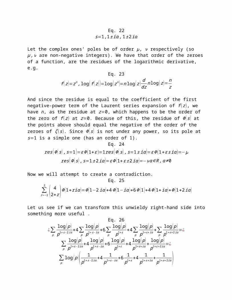
Eq. 22s=1,1± iα ,1±2 iα

Let the complex ones’ poles be of order μ, ν respectively (so μ , ν are non-negative integers). We have that order of the zeroes of a function, are the residues of the logarithmic derivative, e.g.Eq. 23f ( z )=zn , log ( f ( z ) )=log ( zn )=n log ( z )

ddz

n log ( z )=nz

And since the residue is equal to the coefficient of the first negative-power term of the Laurent series expansion of f (z), we have n, as the residue at z=0, which happens to be the order of the zero of f (z) at z=0. Because of this, the residue of Φ ( s ) at the points above should equal the negative of the order of the zeroes of ζ (s). Since Φ ( s) is not under any power, so its pole at s=1 is a simple one (has an order of 1).Eq. 24

res (Φ ( s ) , s=1 )=ϵ Φ(1+ϵ )=1res (Φ ( s ) , s=1± iα )=ϵ Φ(1+ϵ ± iα)=−μ

res (Φ ( s ) , s=1±2iα )=ϵΦ (1+ϵ ±2iα )=−να∈ R ,α ≠0

Now we will attempt to create a contradiction.Eq. 25∑r=−2

2

( 42+r )Φ (1+riα )=Φ (1−2iα )+4Φ (1−iα )+6Φ (1 )+4Φ (1+iα )+Φ (1+2 iα )

Let us see if we can transform this unwieldy right-hand side into something more useful . Eq. 26¿∑

p

log ( p )p1+ϵ−2 iα

+4∑p

log (p )p1+ ϵ−iα +6∑

p

log ( p )p1+ϵ

+4∑p

log ( p )p1+ϵ +iα+∑

p

log ( p )p1+ϵ+2 iα

=¿

∑p

log (p )p1+ ϵ−2 iα

+4 log ( p )p1+ ϵ−iα

+6 log ( p )p1+ϵ

+4 log ( p )p1+ϵ+ iα

+log ( p )p1+ ϵ+2 iα

=¿

∑plog (p )( 1

p1+ϵ−2iα+4 1

p1+ϵ−iα+61p1+ϵ

+4 1p1+ϵ+iα

+ 1p1+ϵ+2 iα )

This looks like the expansion of a linear expression raised to the fourth power Eq. 27∑p

log ( p )p1+ϵ ( 1

p−2 iα+41p−iα +6+4

1p iα+

1p2 iα )=¿

∑p

log ( p )p1+ϵ

(( p iα2 )4+4 ( p

iα2 )3(p

−iα2 )+6 (p

iα2 )2( p

−iα2 )2+4 ( p

iα2 )( p

−iα2 )3+( p

−iα2 )4)=¿

∑p

log ( p )p1+ϵ

( p iα2 + p

−iα2 )4=∑

p

log ( p )p1+ϵ (2cos α2 )

4

≥0

Now, multiply the right-hand side of Eq. 25 by ϵ , let ϵ go to zero, and we getEq. 28−ν−4 μ+6−4 μ±ν=6−8 μ−2 ν ≥0

But here we must remember that μ is a non-negative integer, so in order for this statement to be true, it must be zero. This means there is no pole there, so we have a contradiction. This, with the Result 2, gives us the desired result. Result 4:ζ ( s)≠0 ,∀ s∈C s. t . R (s )≥1

Now we will examine ∫1

∞ θ ( x )−xx2

dx for convergence. First we will try to make the integral that we are concerned with out of something with established properties.Eq. 29

Φ ( s)=∑p

log (p )ps

= limn→∞

∑p

n log ( p )ps =lim

n→∞∑p

n ∑q≤ xi

log (q)− ∑q≤ xi−1

log (q)

ps , p∈¿ xi−1, x i¿

This gives us something with θ ( x ), which is promising.Eq. 30limn→∞

∑p

n ∑q≤ xi

log (q)− ∑q≤ xi−1

log (q)

ps =∫1

∞ dθ ( x )x s

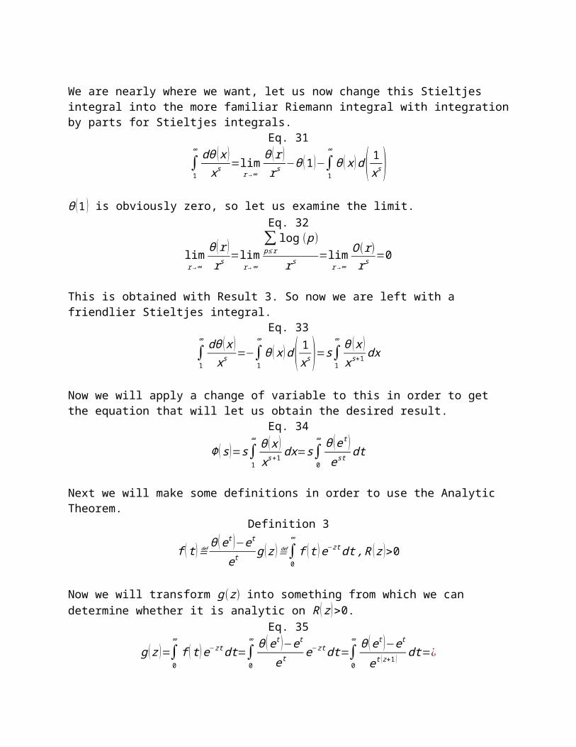
We are nearly where we want, let us now change this Stieltjes integral into the more familiar Riemann integral with integration by parts for Stieltjes integrals. Eq. 31∫1

∞ dθ ( x )xs

=limr→∞

θ (r )rs

−θ (1 )−∫1

∞

θ ( x )d ( 1xs )θ (1 ) is obviously zero, so let us examine the limit.Eq. 32

limr→∞

θ (r )rs

= limr→∞

∑p≤rlog ( p)

r s=lim

r→∞

O(r )r s

=0

This is obtained with Result 3. So now we are left with a friendlier Stieltjes integral.Eq. 33

∫1

∞ dθ ( x )xs

=−∫1

∞

θ ( x )d ( 1xs )=s∫1

∞ θ ( x )xs+1

dx

Now we will apply a change of variable to this in order to get the equation that will let us obtain the desired result.Eq. 34Φ ( s)=s∫

1

∞ θ ( x )xs+1

dx=s∫0

∞ θ (et )est

dt

Next we will make some definitions in order to use the Analytic Theorem.Definition 3f (t )≝ θ (e t )−e t

etg ( z )≝∫

0

∞

f ( t ) e−zt dt ,R ( z )>0

Now we will transform g(z ) into something from which we can determine whether it is analytic on R ( z )>0. Eq. 35g ( z )=∫

0

∞

f ( t ) e−zt dt=∫0

∞ θ (e t )−et

e te− zt dt=∫

0

∞ θ (e t )−e t

e t ( z+1 ) dt=¿

∫0

∞ θ (et )et (z+ 1)

dt−∫0

∞ et

e t( z+1)dt=Φ ( z+1 )

z+1−1z

This shows that g(z ) is analytic by Result 3, and by Result 2 we have that f (t) is bounded, and by definition it resembles a step function and so is continuous almost everywhere. So the Analytic Theorem provides us that ∫0

∞

f ( t ) dt converges.Analytic Theorem:Let f ( t ) ,(t ≥0) be a bounded and locally integrable function and suppose that the function ( z )=∫

0

∞

f ( t ) e−zt dt ,R ( z )>0 extends holomorphically to R ( z )≥0. Then ∫

0

∞

f ( t )dt exists (and equals

g(0)).4Zagier goes onto show the final step here, and then proves the Analytic Theorem; we will instead not prove the Analytic Theorem as it strays too far afield into complex analysis for the purposes of this project.So now we will apply a change of variable to f (t) to get the integral in which we were first interested. Result 5:

x=e t , dxx

=dt

∫0

∞

f ( t )dt=∫0

∞ θ (e t )−et

e tdt=∫

1

∞ θ ( x )−xx2

dx convergent

Now that we have established these five results, we can go on to finish the PNT by showing θ ( x ) x. First we will assume that there is some λ>1 such that θ ( x )≥ λx, for an arbitrarily large x, from this we would haveEq. 36∫x

λx θ ( x )−tt2

dt ≤∫x

λx λx−tt2

dt= limn→∞

∑i=0

n−1 λx−ti¿

ti¿2 (t i+1−t i )t i

¿= λi¿ x ,t i=λ i x ,t i+1=λi+1 x ,1≤ λi

¿ , λi , λi+1≤ λ

limn→∞

∑i=0

n−1 λx−t i¿

ti¿2 (t i+1−ti )=lim

n→∞∑i=0

n−1 λx− λi¿ x

λ i¿2 x2

(λ i+1x−λi x )=¿limn→∞

∑i=0

n−1 λ− λi¿

λ i¿2 (λi+1−λi )=∫

1

λ λ−tt 2

dt>0

But this presents a problem, if any interval with bounds being some integer to λ times that integer is equal to the integral from 1 to λ, then we haveEq. 37∫1

∞ θ ( x )−xx2

dx=limn→∞

∑i=0

n

∫λ i

λi+1 λ−tt 2

dt=limn→∞

∑i=0

n

∫1

λ λ−tt2

dt=limn→∞

n∫1

λ λ−tt2

dt→∞

This contradicts Result 5. By an equivalent argument, we can show that if instead we have λ<1 such that θ ( x )≤ λx, we run into the same contradiction (except this time with −∞).Therefore, we get our final result .Result 6:

θ ( x ) x

Now all that is left is to relate our findings to the prime counting function π (x).4 Zagier, 4

Eq. 38θ ( x )=∑

p≤ xlog ( p )≤∑

p≤ xlog ( x )=π (x ) log ( x )

θ ( x )=∑p≤ xlog ( p )≥ ∑

x1−ϵ ≤ p≤ x

log ( p )≥ ∑x1−ϵ ≤ p≤ x

(1−ϵ ) log ( x )=¿

(1−ϵ ) log ( x ) (π ( x )+O(x1−ϵ))→π ( x ) log ( x ) , as ϵ →0

So we have the long sought after result.PNTπ (x ) log ( x ) xπ (x ) x

log (x )

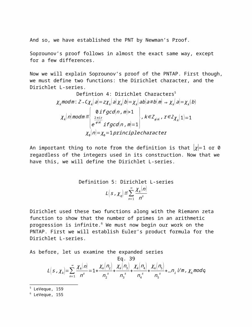
And so, we have established the PNT by Newman’s Proof.Soprounov’s proof follows in almost the exact same way, except for a few differences.Now we will explain Soprounov’s proof of the PNTAP. First though, we must define two functions: the Dirichlet character, and the Dirichlet L-series.Defintion 4: Dirichlet Characters5

χkmodm :Z→C χk (a )=z χk (a ) χk (b )= χk (ab )a≡b (m )⇒ χ k (a )= χ k(b)

χk (n )modm≝{ 0if gcd (n ,m )>1

e2πi rϕ (m ) if gcd (n ,m )=1},k∈Zϕ (m) , r∈Z χk (1 )=1 χ0 (n )= χ0=1 principlecharacter

An important thing to note from the definition is that |χ|=1 or 0 regardless of the integers used in its construction. Now that we have this, we will define the Dirichlet L-series.Definition 5: Dirichlet L-series

L (s , χ q )≝∑n=1

∞ χ k (n )ns

Dirichlet used these two functions along with the Riemann zeta function to show that the number of primes in an arithmetic progression is infinite.6 We must now begin our work on the PNTAP. First we will establish Euler’s product formula for the Dirichlet L-series.As before, let us examine the expanded seriesEq. 395 LeVeque, 1596 LeVeque, 155

L (s , χ k )=∑n=1

∞ χk (n )ns =1+

χk (n2 )n2

s +χ k (n3 )n3

s +χk (n4 )n4

s +χk (n5 )n5

s +…ni ∤m , χ kmodq

Now we will attempt the same step as before, we will find the first prime in the list and obtain Eq. 40χk (p )ps

L ( s , χk )=χk (p )ps

∑n=1

∞ χ k (n )ns

=¿

χk (p )ps

+χk (p ) χ k (n2 )

psn2s +

χk (n3 ) χk ( p )

psn3s +

χk (n4 ) χk (p )

psn4s +

χk (n5 ) χk (p )

psn5s +…=¿

χk (p )ps

+χk (p n2 )psn2

s +χk ( pn3 )psn3

s +χ k ( pn4 )psn4

s +χk ( pn5 )psn5

s +…

Now subtracting Eq. 40 from Eq. 39Eq. 41L (s , χ k )−

χk (p )ps

L ( s , χ k )=(1− χk (p )ps )L ( s , χk )

This removes all the multiples of p from the right-hand side, we would then pick another prime and repeat, and in this way we will sieve out all the primes and solve for L (s , χ q ), and obtainResult 7a:L (s , χ k )=∏

p(1− χk (p ) p−s )−1

Furthermore, in the case of χk= χ0

Result 7b:L (s , χ 0 )=∏

p∤m(1−p−s )−1=∏

p∨m(1−p−s )∏

p(1−p−s )−1=∏

p∨m(1−p−s ) ζ (s)

Now we will show that L (s , χ k ), and L (s , χ 0 )−ϕ (q )q

1s−1 is analytic on

{s∈C :R (s )>0 }. Let Soprounov takes a partial sum from the Dirichlet L-series and changes into the following. I was unable to figure out how he produced this change, so I am forced to take on faith that it is true.Eq. 42

∑n=1

x χk (n )ns

=A ( x )xs

+s∫1

x A ( t )t s+1

d t

Definition 6:A ( x )≝∑

n=1

x

χ k (n )

If χk (n ) is not principal then A ( x ) is bounded by a finite number of roots of unity, as the sum over the mth roots of unity hits zero every ϕ (m ) times. So we will let x→∞ to obtain Eq. 43L (s , χ k )=s∫

1

∞ A ( t )t s+1

dt=s∫1

∞ A (t )t s+1

dt

This is convergent, and therefore analytic for R (s )>0. For the case of χk (n) being principal we can look at Result 7b, or even the definition of L (s , χ k ), and see that it is meromorphic, with only a simple pole at s=1 with residue being Eq. 44∏p∨m

(1−p−1 )=∏p∨m

( p−1p )=∏p∨m

( ϕ ( p)p )=ϕ (m)

m

This gives us all the information needed to sayResult 8:L (s , χ k ) , L ( s , χ0 )−

ϕ (q )q

1s−1

are analytic on {s∈C :R (s )>0 }

Now we will show that θq ( x )=O(x ), but first we must define itDefiniton 7:θq ( x )≝ ϕ (m ) ∑

p≤ xp≡a (m)

log ( p )

This will be easy enough to show. Result 9:θq ( x )≤ϕ (m )θ ( x )=O ( x )⇒ θq(x )=O(x)

Now we will examine Definition 8:

ϕ ( s , χk )≝∑p

χ k ( p ) log pps

Φm ( s )≝∑χk

ϕ ( s , χk )Φm,a (s )≝∑χk

χk (a)ϕ (s , χ k ) , χ k (a)conjugateof χk (a)

We want to show that the Dirichlet L-series has no zeroes for {s∈C :R ( s )≥1 } for any χk, also we will show that Φm ( s )− 1s−1 is analytic there as well.

In order to guarantee our desired result for any χ, we will look at the a new function. Definition 9:L (s )≝∏

χL ( s , χk )

Soprounov takes as given, as will we, that L (1 , χ k)≠0 provided that χk is not principal.So let us now again to the logarithmic derivative of L (s ).Eq. 45L'(s)L ( s)

=

dds∏χ

L ( s , χk )

∏χL (s , χ k )

=

∑χ (L ' ( s , χk )∏

χL ( s , χk )

L ( s , χ k ) )∏χL (s , χk )

=L ' (s , χ k )L (s , χ k )

Therefore, we need only examine the logarithmic derivative of the Dirichlet L-series.Eq. 46

ddslog (L (s , χ k ))=−d

dslog (∏p (1− χ k ( p ) p− s)−1)

We will use the rules of logarithms as before.Eq. 47−L' ( s , χk )L ( s , χk )

=−ddslog (∏p (1− χ k ( p ) p− s)−1)=−d

ds ∑plog ((1− χk ( p ) p− s )−1 )=¿

−∑p

χ k ( p ) p− s log ( p )

(1− χk ( p ) p−s )2

(1− χ k ( p ) p− s)−1=∑

p

χ k ( p ) log ( p )ps− χk (p )

We now use the exact same methods as in the proof for the PNT.Eq. 48∑p

χk ( p ) log (p )ps− χ k ( p )

=∑p

χ k ( p ) log ( p )ps− χk (p )

−χk (p ) log ( p )

ps +¿χ k ( p ) log ( p )

ps=¿¿Φm ( s )+∑

p

χk2 ( p ) log (p )

ps ( ps− χ k ( p ) )

The analyticity for the term on the right is essentially the same as before, so like both authors, we will take it as given.Combined with Result 8, this establishes that the rightmost side is at least meromorphic, that is to say, analytic with a specific set of poles. The rest of the proof of this claim follows indentically to the proof for Result 4.

Result 10:ζ ( s)≠0 ,∀ s∈C s. t . R (s )≥1

Result 8 and Result 10 give Result 11:

Φm,a (s )− 1s−1

asanalytic on {s∈C :R ( s )≥1}.

Now we will show that ∫1

∞ θq ( x )−xx2

dx is convergent.Eq. 49Φm,a (s )=∑

χ k

χk (a )ϕ ( s , χk )=∑χ k

( χk (a )∑p

χ k ( p ) log pps )=¿∑

χ k( χk (a )∑

p

χk (p ) log pps )

The χk (a ) can also be written as χk (a−1mod m), by the multiplicative property of χk, so it works like a filter with χk ( p ) leaving us with only the primes congruent to a modulo m.

Eq. 50∑χ k

χ k (a ) χk ( p )= ∑a−1 p≡1 (m)

1=ϕ (m)

So now we are left with turning Φm,a (s ) into something familiar.Eq. 51∑

a−1 p≡ 1(m)

ϕ(m) log pps = ∑

p≡a(m)

ϕ (m) log pps

This is reminiscent of Φ ( s) from the proof of the PNT, and indeed it can be transformed into an integral in the same manner. So now we have, with a familiar change of variable Eq. 52Φm,a (s )=s∫

1

∞ θq ( x )xs+1

dx=s∫1

∞ θq (e t )est

dx

From here we proceed in the exact same way as in the proof for the PNT, using the Analytic Theorem we get that indeedResult 12:∫1

∞ θq ( x )−xx2

dx convergent

From this point on, the Soprounov proof says nothing new from the Newman proof, so we will cut to the chase and get to the finale.PNTAP

π (x ,q )= xϕ (q ) log x

Now I explain the program by which I will test these results.

Step 1: Make sure that a and q are coprimeThe range of numbers to be tested will be partitioned into testing grounds by the arithemetic progression, so we will see how much is cropped off by the cap of the range.Step 2: Get the distance between the beginning of the final interval and the capStep 3: Calculate the number of prime tests that will be conductedStep 4: Get the value, y of the arithmetic progression for the current testStep 5: If we have gone too far skip to Step 8Step 6: If y is prime add one to the hit countStep 7: Repeat Steps 4-6 until all the tests are doneStep 8: Calculate the estimate according to the PNTAPStep 9: Calculate the absolute errorStep 10: Calculate the relative errorReturn: Number of hits, estimate, absolute error, relative error

def PNTAP_test1(x,q,a): assert gcd(q,a) == 1 finish_q = int(Mod(x,q)) tries = (x-finish_q)/q + 1

hits = 0 for k in range(tries) : y = q*k+a if y > x: break if is_prime(y): hits += 1 estimate = N(x/(euler_phi(q)*log(x))) abs_error = abs(hits-estimate) rel_error = abs_error/hits return [hits,estimate.n(digits=5), \ abs_error.n(digits=5), \ rel_error.n(digits=5)]

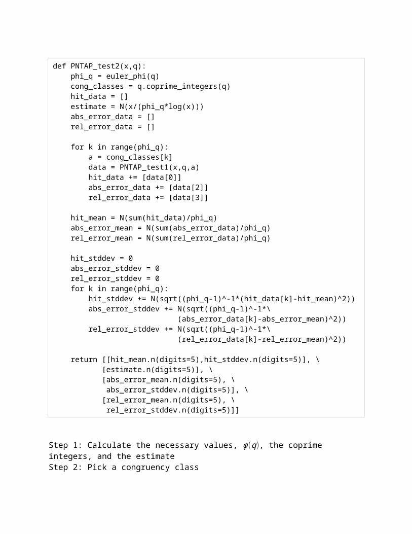
Step 1: Calculate the necessary values, ϕ (q), the coprime integers, and the estimateStep 2: Pick a congruency classStep 3: Obtain data on the given arithmetic progression for all the congruency classesStep 4: Distribute the data among the hit data, absolute errors, and relative errorsStep 5: Calculate the mean for the hit data, absolute errors, and relative errorsStep 6: Calculate the standard deviation for the hit data, absolute errors, and relative errors

def PNTAP_test2(x,q): phi_q = euler_phi(q) cong_classes = q.coprime_integers(q) hit_data = [] estimate = N(x/(phi_q*log(x))) abs_error_data = [] rel_error_data = []

for k in range(phi_q): a = cong_classes[k] data = PNTAP_test1(x,q,a) hit_data += [data[0]] abs_error_data += [data[2]] rel_error_data += [data[3]]

hit_mean = N(sum(hit_data)/phi_q) abs_error_mean = N(sum(abs_error_data)/phi_q) rel_error_mean = N(sum(rel_error_data)/phi_q)

hit_stddev = 0 abs_error_stddev = 0 rel_error_stddev = 0 for k in range(phi_q): hit_stddev += N(sqrt((phi_q-1)^-1*(hit_data[k]-hit_mean)^2)) abs_error_stddev += N(sqrt((phi_q-1)^-1*\ (abs_error_data[k]-abs_error_mean)^2)) rel_error_stddev += N(sqrt((phi_q-1)^-1*\ (rel_error_data[k]-rel_error_mean)^2))

return [[hit_mean.n(digits=5),hit_stddev.n(digits=5)], \ [estimate.n(digits=5)], \ [abs_error_mean.n(digits=5), \ abs_error_stddev.n(digits=5)], \ [rel_error_mean.n(digits=5), \ rel_error_stddev.n(digits=5)]]

Return: hit mean, hit standard deviation, absolute error mean, absolute error standard deviation, relative error mean, and relative error standard deviation

First, we will test the estimate with a particular congruency class (PNTAP_test1).I will use the following arithmetic progressions to explore how far out we need to go to get close results.

TEST 14x+1, x=[103, 105, 107][hits, estimate, mean, absolute error, relative error][80, 72.382, 7.6176, 0.095220] x= 103[4783, 4342.9, 440.06, 0.092004] x= 105[332180, 310210., 21970., 0.066138] x= 107TEST 227x+8, cap=[103, 105, 107, 109] [hits, estimate, mean, absolute error, relative error] [8, 8.0425, 0.042490, 0.0053113] x= 103[543, 482.55, 60.451, 0.11133] x= 105[36912, 34468., 2444.2, 0.066216] x= 107[2824735, 2.6808e6, 143900., 0.050945] x= 109TEST 390x+37, x=[103, 105, 107, 109] [hits, estimate, mean, absolute error, relative error] [8, 6.0319, 1.9681, 0.24602] x= 103[405, 361.91, 43.088, 0.10639] x= 105[27734,25851, 1883.1, 0.067900] x= 107[2119211, 2.0106e6, 108590., 0.051240] x= 109TEST 4105x+16, x=[103, 105, 107, 109] [hits, estimate, mean, absolute error, relative error] [3, 3.0159, 0.015934, 0.0053113] x= 103[405, 361.91, 43.088, 0.10639] x= 105[13835,12925., 909.57, 0.065744] x= 107[1059463, 1.0053e6, 54152., 0.051112] x= 109

We see that, as expected, the relative error decreases as x grows. 27x+8 is odd in that for x = 103 it is unusually accurate, and unlike 105x+16, it can’t be explained as it being a very small number.Now we will try the second fact obtained from the PNTAP (PNTAP_test2) with two arithmetic progressions.

TEST 5m = 27, x=[103, 105, 107][[hit mean,hit stddev],[estimate],[abs error mean,abs error stddev],[rel error mean,rel error stddev]]x=103 [[9.2778, 5.0932], [8.0425], [1.4858, 3.9994],

[0.14958, 0.34342]]x=105 [[532.83, 22.798], [482.55], [50.284, 22.798],

[0.094220, 0.039111]]x=107 [[36921., 170.26], [34468.], [2453.2, 170.26],

[0.066443, 0.0043041]]

TEST 6m = 42, x=[103, 105, 107] [[hit mean,hit stddev],[estimate],[abs error mean,abs error stddev],[rel error mean,rel error stddev]]x=103 [[13.750, 4.0704], [12.064], [1.7181, 3.9359],

[0.11735, 0.25734]]x=105 [[799.08, 24.473], [723.82], [75.259, 24.473], [0.094098, 0.027691]]x=107 [[55381., 93.870], [51702.],

[3679.6, 93.874], [0.066441, 0.0015834]]

The results for this test are less satisfactory, but still we see the means behave like we saw the specific congruency classes from tests 1 through 4.This result is subtly amazing. According to the PNTAP, the number of primes congruent to a number modulo another depends only on the modulus, which means that the primes are evenly distributed among the congruency classes of the multiplicative group of the modulus. This hints at a structure to what otherwise appears to be a randomly distributed set of numbers, the primes.

BibliographyLeVeque, William J. Fundamentals of Number Theory. New York: Dover, 1996.Soprounov, Ivan. A Short Proof of the Prime Number Theorem for Arithmetic Progressions. [http://www.math.umass.edu/~isoprou/pdf/primes.pdf]. 3 March 2010Zagier, D. Newman’s Short Proof of the Prime Number Theorem. [http://mathdl.maa.org/images/upload_library/22/Chauvenet/Zagier.pdf]. 4 March 2010