ˇ ˆ - signals and systems, uppsala university · several of the available ndt methods, such as...

��

��

��

�� and ��

��!"#$��

%��!�&'(&)'�&*%��!�+�,)+&)((*)��,()&-��.��.�.--./ �)&��&,+

�� !�!��"#�$�%��%��%&��'�(��)��*��'

��

*��'� !�!'� ��+��%��,��%��%��-��'�+�� '�� ." '�/"��'� ��'�0�,1�2./32�3$$43../$3�'

13�� 51�(6� ��7�� %�� %��'��5�8�6��%��%��'(��%��%��1�(��8��)��

)��%��%��'�(��%��%�� %� �� '� 9�� %��7��%%��%��%��'�0�� 5�:�;6� �� )��%��'�<��%��%��%��'��)��%��7��'(�� %� �� %��

��'�;��=��%��7��%��>��?��%��'�(��'�9��?��%��'�(��%��)��%��7��)��)�@��%��7��%��'�(��'

�� )��)��)��3��)��%��%��%��

�� !��" ��!�#$�%&'!�� !�� ()%*&+��!��

A��*�� !�!

0��1��B$�3B �40�,1�2./32�3$$43../$3��#�#��#��#��3� �/2�5��#CC��'@�'��C��D��E��#�#��#��#��3� �/26

to Annelie, Elias & Filip

List of Papers

This thesis is based on the following papers, which are referred to in the textby their Roman numerals.

I Engholm, M., Stepinski, T. (2010) Direction of Arrival Estimation ofLamb Waves Using Circular Arrays. Recommended for publication inStructrual Health Monitoring.

II Engholm, M., Stepinski, T. (2010) Adaptive Beamforming for ArrayImaging of Plate Structures Using Lamb Waves. Recommended forpublication in IEEE Transactions on Ultrasonics, Ferroelectrics, andFrequency Control.

III Engholm, M., Stepinski, T., Olofsson, T. (2010) Imaging and Suppres-sion of Lamb Modes Using Multiple Transmitter Adaptive Beamform-ing. In manuscript.

IV Stepinski, T., Jonsson, M. (2005) Narrowband ultrasonic spectroscopyfor NDE of layered structures. INSIGHT, the Journal of The BritishInstitute of Non-Destructive Testing, 47(4):220–225.

V Engholm, M., Stepinski, T. (2005) Designing and evaluating trans-ducers for narrowband ultrasonic spectroscopy. 2005 IEEE UltrasonicsSymposium, 4:2085 - 2088 .

VI Engholm, M., Stepinski, T. (2007) Designing and evaluating transduc-ers for narrowband ultrasonic spectroscopy. NDT & E International,40(1):49–56.

Reprints were made with permission from the publishers.

Contents

1 Introduction . . . . . . . . . . . . . . . . . . . . . . . . . . . . . . . . . . . . . . . . . . 91.1 Non-destructive testing . . . . . . . . . . . . . . . . . . . . . . . . . . . . . . 91.2 Lamb wave imaging . . . . . . . . . . . . . . . . . . . . . . . . . . . . . . . . 101.3 Resonance testing . . . . . . . . . . . . . . . . . . . . . . . . . . . . . . . . . . 121.4 Comments on the author’s contributions . . . . . . . . . . . . . . . . . 141.5 Thesis outline . . . . . . . . . . . . . . . . . . . . . . . . . . . . . . . . . . . . . 14

2 Lamb waves . . . . . . . . . . . . . . . . . . . . . . . . . . . . . . . . . . . . . . . . . . 152.1 Introduction . . . . . . . . . . . . . . . . . . . . . . . . . . . . . . . . . . . . . . . 152.2 Basic model of propagating Lamb waves . . . . . . . . . . . . . . . . . 162.3 Rayleigh-Lamb equations . . . . . . . . . . . . . . . . . . . . . . . . . . . . 172.4 Lamb wave excitation and detection . . . . . . . . . . . . . . . . . . . . 182.5 Experimental estimation of dispersion characteristics . . . . . . . . 212.6 Scattering and reflection of Lamb waves . . . . . . . . . . . . . . . . . 212.A Dispersion compensation . . . . . . . . . . . . . . . . . . . . . . . . . . . . . 23

3 Beamforming . . . . . . . . . . . . . . . . . . . . . . . . . . . . . . . . . . . . . . . . . 253.1 Introduction . . . . . . . . . . . . . . . . . . . . . . . . . . . . . . . . . . . . . . . 253.2 Standard beamforming . . . . . . . . . . . . . . . . . . . . . . . . . . . . . . 263.3 The array steering vector . . . . . . . . . . . . . . . . . . . . . . . . . . . . . 283.4 Array and beam pattern . . . . . . . . . . . . . . . . . . . . . . . . . . . . . . 293.5 Minimum variance distortionless response . . . . . . . . . . . . . . . . 313.6 2D array configurations . . . . . . . . . . . . . . . . . . . . . . . . . . . . . . 333.7 Spatial aliasing . . . . . . . . . . . . . . . . . . . . . . . . . . . . . . . . . . . . 353.8 Correlated signals . . . . . . . . . . . . . . . . . . . . . . . . . . . . . . . . . . 373.9 Robustness against parameter uncertainties . . . . . . . . . . . . . . . 393.10 Processing of broadband signals . . . . . . . . . . . . . . . . . . . . . . . 403.A Phase-mode beamformers . . . . . . . . . . . . . . . . . . . . . . . . . . . . 423.B Multiple signal classification . . . . . . . . . . . . . . . . . . . . . . . . . . 42

4 Previous work on imaging using Lamb waves . . . . . . . . . . . . . . . . 454.1 Array imaging . . . . . . . . . . . . . . . . . . . . . . . . . . . . . . . . . . . . . 454.2 Time-reversal . . . . . . . . . . . . . . . . . . . . . . . . . . . . . . . . . . . . . 464.3 Tomography and distributed sensors . . . . . . . . . . . . . . . . . . . . 474.4 Synthetic aperture focusing techniques . . . . . . . . . . . . . . . . . . 48

5 Array processing of Lamb waves . . . . . . . . . . . . . . . . . . . . . . . . . . 515.1 Introduction . . . . . . . . . . . . . . . . . . . . . . . . . . . . . . . . . . . . . . . 515.2 Wavenumber selectivity . . . . . . . . . . . . . . . . . . . . . . . . . . . . . . 525.3 Paper I - Direction of arrival estimation . . . . . . . . . . . . . . . . . . 53

5.4 Lamb wave imaging . . . . . . . . . . . . . . . . . . . . . . . . . . . . . . . . 545.4.1 Model . . . . . . . . . . . . . . . . . . . . . . . . . . . . . . . . . . . . . . . 545.4.2 Paper II – Single transmitter imaging . . . . . . . . . . . . . . . . 545.4.3 Paper III - Multiple transmitter imaging . . . . . . . . . . . . . . 55

5.5 Conclusions . . . . . . . . . . . . . . . . . . . . . . . . . . . . . . . . . . . . . . . 566 Resonance based methods for the inspection of plate structures . . . 63

6.1 Introduction . . . . . . . . . . . . . . . . . . . . . . . . . . . . . . . . . . . . . . . 636.2 Narrowband Ultrasonic Spectroscopy . . . . . . . . . . . . . . . . . . . 646.3 Paper IV – Experimental evaluation . . . . . . . . . . . . . . . . . . . . . 656.4 Paper V & VI – Transducer design . . . . . . . . . . . . . . . . . . . . . 656.5 Conclusions . . . . . . . . . . . . . . . . . . . . . . . . . . . . . . . . . . . . . . . 66

7 Conclusions . . . . . . . . . . . . . . . . . . . . . . . . . . . . . . . . . . . . . . . . . . 678 Future Work . . . . . . . . . . . . . . . . . . . . . . . . . . . . . . . . . . . . . . . . . . 699 Swedish Summary . . . . . . . . . . . . . . . . . . . . . . . . . . . . . . . . . . . . . 71

9.1 Oförstörande provning . . . . . . . . . . . . . . . . . . . . . . . . . . . . . . . 719.2 Lamb vågor . . . . . . . . . . . . . . . . . . . . . . . . . . . . . . . . . . . . . . . 729.3 Resonansprovning . . . . . . . . . . . . . . . . . . . . . . . . . . . . . . . . . . 72

10 Acknowledgements . . . . . . . . . . . . . . . . . . . . . . . . . . . . . . . . . . . . 75Bibliography . . . . . . . . . . . . . . . . . . . . . . . . . . . . . . . . . . . . . . . . . . . . 77

1. Introduction

Plate structures are everywhere in the world around us. Cars, ships, airplanes,and pressure vessels are only a few examples of vehicles and engineered struc-tures consisting of a considerable amount of flat or slightly curved plates.These are often required to have a significant life span. For instance, it is notuncommon for airplanes to be in service for over 20 years. During that time,the high safety standards required by governments and consumers need tobe complied, requiring frequent maintenance and inspection of critical areas.This, among many other applications, has triggered the development of testingmethods that can assess the state of a structure or material without affectingits functionality, so called non-destructive testing (NDT).

1.1 Non-destructive testingDuring the last century, a large number of NDT techniques were developed.One technique that has proven to be very versatile for many different appli-cations is the use of high frequency, or ultrasonic, elastic waves. Ultrasonicinspection is commonly performed by transmitting an ultrasonic pulse into theinspected object, which is reflected, or backscattered, at discontinuities withinobject. These echoes are received and analysed in time to search for echoesthat can indicate the presence of defects.

The generation and detection of ultrasonic waves is performed using trans-ducers that provide the means for converting electric signals into elastic wavesand vice versa. This transduction can be accomplished using a number ofdifferent physical principles. For example, piezoelectric transducers convertelectrical energy to mechanical energy in a piezoelectric element, in contrastto electromechanical acoustic transducers (EMAT) that generate and detectelastic waves in a metallic object through magnetic fields, making the actualtransduction occur inside the object.

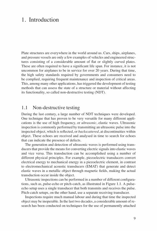
Ultrasonic inspections can be performed in a number of different configura-tions, such as, pulse-echo or pitch-catch, as illustrated in Figure 1.1. A pulse-echo setup uses a single transducer that both transmits and receives the pulse.Pitch-catch setups, on the other hand, use a separate receiving transducer.

Inspections require much manual labour and during that time the inspectedobject may be inoperable. In the last two decades, a considerable amount of re-search has been conducted on techniques for the use of permanently attached

9

devices capable of continuous monitoring of structures, so called structuralhealth monitoring (SHM). The benefits of such an approach are improvedsafety and reduced costs by early warning of potential problems [1]. Thiscould also reduce the frequency of manual inspections that can be extremelytime consuming if large areas require inspection. The work presented in thisthesis is highly relevant for, but not limited to, SHM.

Figure 1.1: Pulse based inspections. Pulse-echo setup (left) and pitch-catch setup(right).

1.2 Lamb wave imagingSeveral of the available NDT methods, such as eddy current testing, can onlydetect defects directly under the probe. Although precise localization and, inmany cases, high sensitivity can be achieved, it makes inspection of large platestructures extremely time consuming. An alternative to these types of methodsis using ultrasonic guided waves. Guided waves can potentially propagate overlong distances and can therefore be used for rapid inspection of large areas ofan object. Examples of applications which benefit from guided waves includelong range testing of pipes and rails [2]. A literature survey and summary ofguided wave applications can be found in [3].

Guided waves in plate structures, so called Lamb waves, have been of con-siderable interest for NDT during the last few decades. Probably the earliestexperimental work on ultrasonic Lamb waves was done by Worlton who pro-posed their application for NDT in 1961 [4]. In the same manner as for bulkwaves illustrated above, Lamb wave inspections can be performed in eitherpulse-echo, as illustrated in Figure 1.2, or pitch-catch configuration.

Figure 1.2: Principle of pulse-echo Lamb wave inspection. The guided wave propa-gates in the plate and is reflected at discontinuities.

Applications employing Lamb waves for NDT include testing and eval-uation of adhesive bonds [5, 6, 7], isotropic plates [8, 9, 10], and compos-

10

ites [11, 12, 13]. Furthermore, Lamb waves ability to propagate over long dis-tances, and thereby enabling wide area coverage, has resulted in a significantamount of research on their application in SHM. A review of work concerningLamb wave structural health monitoring can be found in [14].

The first part of this thesis concerns a particular application of Lamb waves:imaging. Imaging in general is the representation of an object’s externals orinternals in the form of an image. Through the ability of Lamb wave to prop-agate over large distances, an array of transducers capable of transmitting andreceiving Lamb waves in arbitrary directions, enables acquisition of backscat-tered data from a large area around the array. An illustration of such a setup isshown in Figure 1.3. The backscattered waves will consist of reflections fromboundaries, such as edges, welds, or defects. Processing of such data enablesestimation of amplitudes and positions of scatterers in the region of interest(ROI). However, Lamb wave propagation and interaction with discontinuitiesis very complex, which complicates acquisition and the following reconstruc-tion of an accurate image.

Figure 1.3: One or multiple elements in an array generate Lamb waves that propagatein the plate. The array elements receive the backscattered signals enabling estimationof the position and size of a potential defect.

In traditional applications using arrays, as for instance in radar and sonar,as well as in ultrasonic testing in bulk materials, one dimensional (1D) ar-rays are commonly used. Such arrays consist of elements along a line. Arraysused for the type of inspection, or monitoring, considered in this thesis shouldpreferably allow omni-directional coverage. As will be discussed in Chapter 3,omni-directional coverage requires the use of two dimensional (2D) arrays,that is, arrays that have its elements distributed in two dimensions, for exam-ple circular arrays. However, a significant number of elements in the 2D arrayis required to achieve sufficient resolution. Previous work on imaging of Lambwaves has mainly been focused on basic array processing methods that maynot fully exploit the potential of the setup. In this thesis, more advanced meth-

11

ods are considered that better utilize the available data to improve resolutionand reduce noise in the resulting image.

1.3 Resonance testingThe first section described the use of ultrasonic pulses to interrogate the in-side of an object in the search of defects. An alternative to the pulse-based,time domain, techniques are methods concerning the extraction of informationcontained in an object’s natural modes of vibration. The resonance frequenciesare directly related to the structure’s material properties, such as thickness andelasticity. Defects in a structure will affect its vibrational modes which can beused to assess its condition.

The most common application for this type of methods is the inspection ofbonded joints and composites. Defects, such as disbonds or voids in adhesivelayers, are in many cases readily detected with these techniques since such de-fects cause a significant change in the structure’s vibrational modes. The basicprinciple of resonance tests is to measure the electrical impedance responseof a transducer that is acoustically coupled to the structure as illustrated inFigure 1.4. Acoustic coupling is achieved through a thin layer of couplant,for example water. Resonances occur at frequencies where the transducer’simpedance reaches minima. Changes in the structure directly under the trans-ducer will affect the electrical impedance of the transducer, which can be usedto detect defects. Compared to Lamb waves that propagate in the plate, thistype of inspections are local.

Figure 1.4: A transducer is coupled to the inspected structure by a thin layer of, e.g.water. The transducer is excited by a frequency sweep or a fixed frequency. Changesin resonance frequency or complex transducer impedance are used to detect defects.

This principle can be used in two ways. Instruments, such as, the Fokkerbond tester, tracks the transducer’s resonance frequency for changes thatindicates anomalies in the structure. Other instruments, for example the

12

BondaScope 31001, tracks the complex electrical impedance at a singlefrequency and displays it in the complex impedance plane.

The second part of this thesis concerns the evaluation of the compleximpedance approach. Considerations concerning frequency selection andproperties of the transducers to maximize the sensitivity of the measurementare presented.

1NDT Systems, Inc.

13

1.4 Comments on the author’s contributionsThe author’s contributions to the respective papers are summarized below.

I Ideas (except phase-mode approach), experimental setup design andconstruction, software implementation, simulations, measurements, in-terpretation, major part of writing

II Ideas, experimental setup design and construction, software implemen-tation, simulations, measurements, interpretation, major part of writing

III Ideas, experimental setup design and construction, software implemen-tation, simulations, interpretation, major part of writing

IV Measurements, parts of software implementation, simulationsV Idea, software implementation, simulations, interpretation, major part

of writingVI Idea, software implementation, simulations, interpretation, major part

of writing

1.5 Thesis outlineSince most readers interested in this thesis are probably familiar with eitherLamb waves or beamforming methods, but not both, the first two chaptersprovide a basic introduction into the subjects.

This thesis is organized as follows:

• Chapter 2 gives an overview of important properties of Lamb waves rele-vant for the work.

• Chapter 3 introduces the basic concept of both conventional beamform-ing and adaptive methods. It also serves as a preparation for Chapter 5 bybringing to attention some issues that need to be addressed when employ-ing these techniques for active array imaging.

• Chapter 4 provides a short overview of important previous work on Lambwave imaging with emphasis on arrays.

• Chapter 5 explains the issues related to Lamb waves that need to be con-sidered when using adaptive methods on Lamb waves and the steps thatresulted in Papers I, II and III.

• Chapter 6 introduces the narrowband ultrasonic resonance spectroscopytechnique and the contributions made in Papers IV, V and VI.

• Chapter 7 summarizes the conclusions .• Chapter 8 suggests future work.

14

2. Lamb waves

2.1 IntroductionIsotropic elastic bulk media support two types of wave motion, longitudinaland shear. A longitudinal wave has its displacement in the direction of propa-gation, while a shear wave has its displacement perpendicular to the directionof propagation. These waves propagate with different velocities, where the ve-locity of the shear wave, cS , is lower than the longitudinal wave’s velocity, cL.

Consider a harmonic plane wave, s(x, t), propagating along the x-axis ina medium. Harmonic refers to a wave consisting of a single angular fre-quency, ω. Waves having constant phase over a plane, in this case perpen-dicular to the x-axis, are referred to as plane waves. The wave at position xand time t, can be described in complex form as

s(x, t) = Aej(ωt−kx) (2.1)

where k is the wavenumber and A is the amplitude of the wave. The wavenum-ber k is related to the phase velocity of the wave, cp, as

k = ω/cp. (2.2)

Henceforth, the harmonic dependency ejωt will be assumed implicitly fornotational convenience.

The longitudinal and shear waves mentioned above both have frequencyindependent phase velocities, which results in linear frequency-wavenumberrelationships. This means that these waves are non-dispersive and the shapeof the waves will be preserved during propagation.

When the dimensions of the media approach the order of the wavelength, itstarts behaving as a wave guide. Waves propagating in a wave guide are calledguided waves. Such waves in infinite elastic plates were first described andanalyzed by Horace Lamb in 1917, and they are therefore called Lamb waves.In application oriented publications, a commonly occurring name for guidedwaves in plates are guided Lamb waves. In contrast to bulk waves, guidedwaves are dispersive, i.e. they have frequency dependent dependent velocity.This means that the shape of a wave packet changes during propagation.

Another property Lamb waves shares with other types of guided waves isthe possible existence of multiple propagation modes. These so called Lambmodes follow different dispersion relationships, i.e., the relation betweenphase velocity and frequency depends on the mode. As a consequence, there

15

may be several propagation velocities even for a single frequency. Dependingon the thickness of the plate and the frequency of the wave, anywhere fromtwo to infinitely many Lamb modes can propagate in the plate.

Compared to Rayleigh waves, which propagate in a shallow zone belowthe surface of a material, Lamb waves have through-thickness displacementpermitting detection of defects both within and close to the surface of theplate. This, along with their ability to propagate over long distances, makethem suitable for both inspection and monitoring of plate structures.

Beside Lamb waves, there is another type of guided wave modes in platescalled shear horizontal (SH) modes [15]. These modes propagate with dis-placements in-plane, i.e. parallel to the plate, compared to Lamb waves whichhave only out-of-plane, i.e. perpendicular to the plate, components perpendic-ular to the direction of propagation. The SH-waves have not been given anyspecial consideration in this work since the setup used for the experimentscannot detect this type of wave motion.

2.2 Basic model of propagating Lamb wavesConsider an isotropic homogeneous plate of thickness d illustrated in Fig-ure 2.1. In this plate, harmonic waves of angular frequency ω can propagatein a number of Lamb modes. Let cp,n(ω) denote the phase velocity of the n-thmode at ω, yielding the corresponding wavenumber kn(ω) = ω/cp,n(ω).

Consider now a line source producing a harmonic surface stress perpen-dicular to the plate at u3 = 0, with u3 indicated in the figure, and let T (ω)denote the amplitude of the stress. The excitation of mode n from the surfacestress is modeled by the transfer function Hn(ω). The normal displacementon the plate surface of the resulting wave propagating in the u3 direction isthen given by

Un(ω, u3) = Hn(ω)T (ω)e−jkn(ω)u3 . (2.3)

The total displacement at u3 is given as a superposition of the modes

U(ω, u3) =∑n

Hn(ω)T (ω)e−jkn(ω)u3 , (2.4)

where the sum ranges over the possible modes at frequency ω.The above scenario corresponds to a line source. A better representation of

the small array elements considered in this work is to consider them as point-like sources. Such a source, producing an out-of-plane harmonic stress withamplitude T (ω) at the origin, generates a cylindrical wave that will divergeradially as it propagates. Its displacement field can be approximated by

U(ω, r) =∑n

1√rHn(ω)T (ω)e−jkn(ω)r, (2.5)

16

where r is the distance to the source. Note the difference in notation for thetransfer function, Hn(ω), which indicates that a point source is considered.

The model (2.5) predicts how the out-of-plane displacement depends on thestress excitation and how it is affected by the distance r from the source. Notethat in order to obtain U(ω, r) the dispersion characteristics, kn(ω), has to bedetermined, as well as the number existing modes and the transfer functionHn(ω). The following sections will give a short introduction to these impor-tant properties of Lamb waves that are relevant to the work presented in thisthesis.

Figure 2.1: One dimensional plate model. A surface stress T (ω) normal to the plateexcites propagating modes in the plate.

2.3 Rayleigh-Lamb equationsConsider again the plate introduced in the previous section with thickness d.Lamb modes can be either symmetric, i.e. with symmetric wave shapes acrossthe plate thickness, or antisymmetric, i.e. with antisymmetric wave shapes. Awavenumber, k, of a possible propagating Lamb mode for a given frequency,ω, is a real solution to the Rayleigh-Lamb characteristic equations [15]

tan(qd/2)

tan(pd/2)= − 4k2pq

(q2 − k2)2for symmectric modes (2.6)

tan(qd/2)

tan(pd/2)= −(q2 − k2)2

4k2pqfor antisymmectric modes (2.7)

where p2 = (ω/cL)2−k2 and q2 = (ω/cS)2−k2, cL is the longitudinal wavevelocity and cS is the shear wave velocity.

As mentioned earlier, for a given frequency there are typically severalwavenumbers satisfying the Rayleigh-Lamb equations (2.6) and (2.7), eachcorresponding to a separate mode. For the lowest frequencies there are twosolutions, the fundamental (anti-)symmetric (A0)S0 mode. The successivesolutions for increasing frequencies, result in higher order modes. These arenumbered (A1)S1, (A2)S2, and so forth. The frequency limit above which aparticular mode can exist is called the mode’s cut-off frequency. To allow asimple notation in equations a single index, n = 0, 1, 2, 3, . . ., is used toidentify modes S0, A0, S1, A1, . . ., in this thesis.

17

The group velocity is the velocity at which the envelope of a narrowbandwave packet propagates. It is related to the wavenumber as

cg =dω

dk. (2.8)

The group velocity provides insight into the amount of dispersion each modeis subjected to in various frequency bands. At frequencies where the groupvelocity changes sharply the wave is severely dispersed, while a frequencyregion with constant group velocity indicates low dispersion. As mentionedearlier, for non-dispersive media there is a linear relationship between the fre-quency and wavenumber, making the group velocity equal to the phase veloc-ity cp = cg .

Figure 2.2 shows the phase and group velocities of the solutions to (2.6)and (2.7) for a 6 mm aluminium plate. Its material properties correspond to aplate used in the experiments presented in Paper I–III. The effect of dispersionis illustrated in Figure 2.3. A bandpass filtered 1 cycle 300 kHz sinusoidalstress at u3 = 0, shown in the first plot, is used to simulate propagation oftwo modes, S0 and A0, in a 6 mm Al plate using (2.4). For simplicity it isassumed that both modes are excited equally, that is, H0(ω) = H1(ω). Thewavenumbers, kn(ω), used for the simulation are given by the dispersion char-acteristics in Figure 2.2. The frequency band between the dash-dot lines is thebandwidth of the signal. The plots in the lower part of Figure 2.3 show the sur-face displacement at distances 0.2 and 0.4 m. It can be seen that the S0 modeis severely dispersed, while the shape of the A0 mode is only slightly alteredby the propagation. This can be explained by observing in Figure 2.2 that thegroup velocity of the A0 mode is almost constant in the frequency band of thesignal.

2.4 Lamb wave excitation and detectionMost of the work on plate inspection using Lamb waves relys on conceptsassuming a single dominant mode which enables estimation of time-of-flightand beamforming without significant interference from other Lamb modes.This work has depended on the development of transducers and instrumenta-tion that are mode selective.

Perhaps the simplest way of exciting a single Lamb mode is by generat-ing an ultrasonic wave with a suitable angle of incidence into the plate [15],which is the basic principle of angle beam transducers. Angle beam trans-ducers consist of a transducer and a plastic wedge that gives the generatedwaves a particular incidence angle to the plate, resulting in a directional wave.The angle of the incident wave and its frequency determine the amplitudes ofthe excited modes, and can therefore enable mode selectivity [15]. The ampli-tudes of excited Lamb modes are in general frequency dependent and highly

18

0 500 1000 15000

2000

4000

6000

8000

10000

Frequency [kHz]

Phas

e ve

loci

ty (

c p) [m

/s]

S0

S1

S2

S3

A0

A1

A2

A3

0 500 1000 15000

1000

2000

3000

4000

5000

6000

7000

Frequency [kHz]

Gro

up v

eloc

ity (

c g) [m

/s] S

0S

1 S2

A0

A1 A

2

A3

Figure 2.2: Dispersion curves for 6 mm Al plate. Phase velocity (top) and groupvelocity (bottom). Dash-dot lines show the frequency band of the signal in Figure 2.3.

affected by the transducer type. This is the reason for using mode and sourcedependent transfer functions Hn(ω) and Hn(ω) in Section 2.2, as the excita-tion will couple to various modes differently. For instance, a small transducermay be approximated by a point source. Other transducers may be better ap-proximated using line sources. The analytic expressions required to calculatethe transfer functions can be found in, for example, [16, 15, 17].

An alternative to angle beam transducers are interdigital transducers (IDT).These transducers consist of finger shaped metallic coatings on a piezoelectricsubstrate as in a surface acoustic wave (SAW) device. The wavelength of theresulting Lamb wave is determined by the distance between the fingers ofthe transducer and the input signal frequency. Experimental work evaluatingthe use of IDTs for Lamb wave generation and reception include [18, 19, 20].Since these transducers generate highly directional waves they are not suitablefor applications where omni-directional coverage is desired.

Omni-directional mode selectivity requires different methods. For array ap-plications, Wilcox used a circular array of EMAT transducers to excite an

19

0 1 2 3 4

x 10−4

−1

0

1

u3 = 0 [m]

0 1 2 3 4

x 10−4

−1

0

1

u3 = 0.2 [m]

0 1 2 3 4

x 10−4

−1

0

1

u3 = 0.4 [m]

S0

A0

t [s]

Figure 2.3: Normal surface displacement at various distances when the excitationsignal is a bandpass filtered 300 kHz 1 cycle sinusoid. Two modes are simulated, theS0 and A0 mode having equal power. The A0 mode is almost non-dispersed whereasthe S0 mode is severely dispersed.

omni-directional S0 mode [21, 22]. In [23], Giurgiutiu proposed an approachwhere the size of piezoelectric elements was selected to improve the modeselectivity for a certain frequency range.

In summary, most important in these methods is frequency selection toachieve mode selectivity, which comes at the price of limited bandwidth. Asa consequence, a design relying on this idea may yield signals that have toopoor range resolution for certain applications. This may hold for instance inimaging applications. As discussed in Section 2.3, the choice of frequencyalso affects the dispersion of the wave packet. Thus, there is a trade-off be-tween mode selectivity and low dispersion, and bandwidth. However, using atransducer that is mode selective in a low dispersive frequency band simplifiesdirect interpretation of the received signals.

For more information concerning different transducer techniques for Lambwave generation and detection see the review articles [3, 13, 14], and the ref-erences therein.

20

2.5 Experimental estimation of dispersioncharacteristicsIt should be apparent from the discussions in the previous sections, that thedispersion characteristics play an important role in plate inspection usingLamb waves.

To take dispersion into account and achieve sufficient performance in rangeestimation, accurate estimates of the dispersion characteristics of the structureare required. The adaptive beamforming approaches considered in this workare particularly sensitive to errors in phase velocity, see Section 3.9.

For homogeneous isotropic structures it may be sufficient to solve theRayleigh-Lamb equations in (2.6) and (2.7), using estimates of the bulk wavevelocities. More complex structure consisting of, for example, anisotropicmaterials or multiple layers, may require a more direct approach to theestimation of the dispersion characteristics. Several approaches have beenpresented for experimental determination of the the frequency dependentphase velocities of multimodal Lamb waves.

Alleyne and Cawley [24] proposed an approach using a two dimensionalFFT on signals received at regular distances from a broadband source to esti-mate the wavenumbers for each frequency. By first performing a temporal FFTon each of the received signals, followed by a spatial FFT over the receviedsignals for each frequency, their method results in a frequency-wavenumberspectrum.

An example of this estimation for the 6 mm Al plate, used in Papers I–III,can be seen in Figure 2.4. The experimentally estimated dispersion curves forthe different modes are clearly seen and can be compared to the theoreticalcurves by presenting the solutions in Figure 2.2 as wavenumbers instead ofphase velocities, k = ω/cp.

Other approaches for estimating dispersion characteristics include time-frequency analysis, such as the short-time Fourier transform (STFT). Suchmethods allow the phase velocities for the different modes to be estimated us-ing a broadband source and a single receiver at fixed positions. Some of thesemethods are reviewed and evaluated by Niethammer et al. [25].

2.6 Scattering and reflection of Lamb wavesWhen performing inspection using ultrasound in, for example, a pulse-echoor pitch-catch setup, the presence and amplitude of the reflected or transmit-ted signals provide valuable information concerning the state of the object.Unfortunately, for Lamb waves the reflection at boundaries are often verycomplicated compared to, for example, bulk waves. Both naturally occurringboundaries, such as plate edges or welds, and defects, such as corrosion pitsor cracks, may affect the shape of the wave on reflection. One reason for this

21

0 200 400 600 800 10000

500

1000

1500

Frequency [kHz]

Wav

enum

ber

[1/m

]S

0 S1

S2

A0

A1

A2

Frequency [kHz]

Wav

enum

ber

[1/m

]

0 200 400 600 800 10000

500

1000

1500

Figure 2.4: Dispersion curves for 6 mm Al plate used in the experiments. Theoretical(top) and experimental (bottom) frequency-wavenumber spectra.

is that the reflection and transmission coefficients are frequency dependent formany types of discontinuities [10, 26]. Furthermore, depending on the charac-teristics of the boundary and the frequency content of the Lamb wave, modeconversion could occur between modes of different order, e.g. A0 to A1, aswell as between antisymmetric and symmetric modes [15]. Recall from Sec-tion 2.4 that the initial wave generated by a transmitter can consist of multiplemodes that, on reflection, are split into even more modes and hence the re-ceived wave becomes more complex. An important consequence of this isthat methods used for detection or estimation of Lamb waves have to be ro-bust with respect to variations in the shape of the wave. Detailed studies ofthe mode conversion phenomenon at, for example, plate edges can be foundin [27], and for notches in [28, 29].

Mode conversion at defects could, if handled correctly be used as a sourceof information, and should therefore not be seen purely as a problem. In forexample [26, 30], the presence of converted modes was proposed to indicate a

22

defect. The amplitude of a converted mode was also used to estimate the sizeof cracks.

2.A Dispersion compensationKnowledge of the dispersion characteristics for a particular mode enablesstraightforward compensation of the dispersive effects from propagation forthat mode. This can allow a wider bandwidth of the signals as long as suffi-cient mode selectivity can be achieved. In [31], Wilcox provides a thoroughanalysis of basic dispersion compensation and also proposes a computation-ally efficient approach to the problem.

The most straightforward way of compensating is to simply phase shift eachfrequency component corresponding to a certain propagation distance. Thiscan be performed for a distance z at t = 0 as

h(z) =

∫ ∞−∞

G(ω)ejkn(ω)zdω. (2.9)

where G(ω) is the Fourier transform of a dispersed signal. Assuming thatt = 0 was the excitation time, this has removed the dispersion by backpropa-gating the signal to its initial position.

The direct calculation of the integral in (2.9) for each distance is com-putationally demanding. In [31] Wilcox used the inverse FFT to transformdata from wavenumber domain into the spatial domain. Since the frequency-wavenumber relationship is non-linear in the dispersive case, the frequencydomain data needs to be interpolated into equally spaced wavenumber pointsbefore applying the inverse FFT. This approach is of course computationallymuch more efficient.

23

3. Beamforming

3.1 IntroductionBeamforming is the concept of forming directional beams using an aperture.For example, the dish of a satellite antenna provides directionality by reflect-ing energy from a specific direction to the head, which contains the actualantenna. To receive signals from other directions, mechanical steering of thedish is required.

In radar, directional steering can be achieved by rotation of the antenna al-lowing scanning of one direction at a time. Being an active technique, whichboth transmits and receives data, it is capable of range resolution. For otherapplications mechanical steering might be impractical and sometimes impos-sible. For SHM or NDT a much more convenient alternative would be to usearrays of sensors, which enable electronic steering of the received signals.

Arrays usually consist of a set of identical transducers, although transmit-ting and receiving array elements can be of different types. An active setupcan be of basically any geometry and combination of transmitting and receiv-ing elements as seen in Figure 3.1. It is also common that the instrumentationis capable of switching between transmission and reception of the elementsduring a single excitation cycle to both transmit and receive using the sameelement.

In array imaging, one or several transmitters are excited using a probingsignal, in this thesis an elastic wave, which is transmitted into the object. Thepropagating elastic wave is reflected at boundaries, such as defects, and thosereflections are received by the array. Knowledge of the position of the trans-mitter, the instant of excitation, and the phase velocity in the material enablesboth angle and range estimation. The backscattered data is then processed toreconstruct an image of the internals of the object in the region-of-interest(ROI).

It is worth noting that for inspections using active setups, where the excita-tion and reception procedure can be repeated indefinitely, the array is merely aconvenience. The key to the processing algorithms is the spatially distributedmeasurement positions of the array that allow spatial resolution. For a station-ary environment there is nothing in the actual processing step preventing theacquisition to be performed sequentially by manual positioning of two trans-mitting/receiving elements on a set of points forming a virtual array.

A dataset of backscattered signals acquired using a single transmission willbe referred to as a single snapshot. When a dataset is acquired using separate

25

Figure 3.1: General setup for array imaging of plates. The acquisition is repeated foreach transmitting element.

transmissions from multiple spatial position, such as an array of transmittingelements, it will be referred to as multiple snapshot. This distinction will beimportant in the discussion on correlated signals in Section 3.8.

3.2 Standard beamformingThe simplest and most widely used technique for beamforming is the delay-and-sum (DAS) beamformer, or simply, the standard beamformer. Its princi-ples are simple; by applying delays on the received data from each receiverelement prior to summation, the output from the beamformer can be steeredin a certain direction. Signals impinging from the steered direction will addup constructively, while interfering signals from other directions will gener-ally be reduced. This is referred to as coherent averaging of signals from thesteered direction.

A typical array setup is illustrated in Figure 3.2 for a so-called uniformlinear array (ULA). A ULA is a linear array with equispaced array elements.The figure illustrates a plane wave, s(t), impinging on the array. The resultingsignals acquired from each element are shown in Figure 3.3.

Let gm(t) denote the signal received by element m. All signals received bythe array can be ordered in a column vector g(t) as

g(t) = [g0(t) g1(t) · · · gM−1(t)]T . (3.1)

In this example element 0 is used as a reference and it receives the signalg0(t) = s(t − T ), where T is a time delay. Element 1 receives the signal τ1seconds later, s(t − T − τ1). Element 2 receives s(t − T − τ2), etc. To steerthe array to the direction of the signal, each channel m has to be time-shiftedby τm s, which corresponds to the delay caused by the time-of-flight between

26

the elements for a particular direction θ. The delayed and aligned signals areshown in Figure 3.3. This is beamforming on reception, but the same conceptalso allow steering of transmitting signals. Steering on transmission will directthe transmission power to a particular direction.

Figure 3.2: Plane wave impinging on a ULA from direction θ. Element 0 is used asreference position.

Figure 3.3: Left: The signals received by each array element. Right: Applying time-shifts aligns signals from a particular direction before summation.

In general, the receivers will pick up signals from several directions simul-taneously. If θ is the direction of current interest, the signals arriving fromother directions are considered as interfering signals and the correspondingsources are often called interferers. Moreover, the acquired signals are typi-cally noise corrupted, with the noise sources being, for instance, thermal noisein the electronics. In array processing it is common to define the measuresignal-to-interference and noise ratio (SINR)

SINR =Psignal

Pnoise + Pinterference, (3.2)

where P denotes the power of the respective components.Steering the transmitted signal improves the SINR for potential reflectors

in the steered direction. Reflected signals from the steered direction will have

27

higher amplitudes, which will improve the signal-to-noise ratio (SNR) in theelectronics. A disadvantage with this is that the focused transmission has tobe repeated for all angles in the ROI. These datasets are often processed inde-pendently using DAS.

An alternative to steering on transmission is to excite each transmitter sep-arately and acquire multiple snapshots of backscattered signals. This datasetcan then be used for synthetic focusing during post-processing by performinga DAS operation on the data from each transmission and average the results.This will improve the SINR, however, since the noise level of the receivingelectronics is fairly independent of the signal level, acquiring backscatteredsignals from single excitations results in lower SNR compared to when steer-ing on transmission. Furthermore, detection of small amplitudes may also belimited by the dynamic range of the AD-converters in the receiver.

3.3 The array steering vectorFor narrowband signals1 the delays can be implemented as simple phase-shifts, allowing a simple mathematical description through the so called ar-ray steering vector or array manifold vector, which is the most fundamentalmathematical model of an array.

The steering vector consists of phasors corresponding to the relative phase-shifts for each array element related to the propagation over the array for aplane wave impinging from a particular direction.

Thus for narrowband signals with center frequency ω, the steering vectorfor a M element ULA can be written as

a(θ) =[1 e−jωτ1(θ) · · · e−jωτM−1(θ)

]T, (3.3)

where τm(θ) is the relative propagation time for signals from angle θ, whereelement 0 is used as a reference.

For a M element ULA with element spacing d, the exponential for eachelement m is given by

ωτm(θ) = mkd sin θ, (3.4)

where k is the wavenumber. Insertion in (3.3) gives

a(θ, k) =[1 e−jkd sin θ · · · e−j(M−1)kd sin θ

]T. (3.5)

For most traditional applications, the wavenumber is directly given by fre-quency and is therefore usually omitted as a parameter for narrowband sig-

1A narrowband signal can be modeled as Re{s(t) exp(jωt)}, where s(t) is a slowly varyingcomplex envelope. Slowly varying in this case means that it can be considered constant duringthe propagation over the array.

28

nals, as a(θ). Recall from Chapter 2 that Lamb waves are multimodal with thepossibility of multiple wavenumbers for each frequency component. There-fore, in order to separate different modes, a 2D wavenumber is used to repre-sent an impinging signal, k = [kx, ky]

T , or in polar coordinates (θ, k), wherekx = k cos(θ) and ky = k sin(θ).

Using the steering vector, a model of the received narrowband signals g(t)can be written as

g(t) = a(θ, k)s(t) + n(t), (3.6)

where n(t) is a superposition of noise and potential interferers. The steeredoutput for narrowband signals can be written as

y(t) =1

MaH(θ, k)g(t) (3.7)

where H is the conjugate transpose, and M normalizes the output to unit gainfor the steered direction.

The effect of the beamforming operation becomes obvious when inserting(3.6) into (3.7)

y(t) =1

MaH(θ, k)g(t) =

1

MaH(θ, k) (a(θ, k)s(t) + n(t))

= s(t) +1

MaH(θ, k)n(t), (3.8)

using that aH(θ, k)a(θ, k) = M . Hence, the output of the beamformer is s(t)plus the contribution from the incoherently averaged noise and interference.

It is necessary to make a distinction between sources that can be consideredas near the array, and sources far from the array. A signal originating from thevicinity of the array, can be considered as near-field if the propagating wavehas a curved wavefront. This means that the phase delays between the arrayelements are not only a function of angle, but also of range. Sources furtheraway from the array are in the far-field if the impinging wave has a planewavefront, a plane wave, making the phase delays between the array elementsapproximately functions of only angle. This is particularly important whenusing adaptive algorithms in near-field as described in Chapter 5.

3.4 Array and beam patternThe standard beamformer described above does not allow perfect isolation ofsignals from a particular direction. That is, signals outside the steering an-gle can cause significant interference. An important tool in characterizing theperformance of an array is the array pattern. It is the output of an unsteered

29

standard beamformer for incoming plane waves of unit amplitude over a rangeof angles and wavenumbers.

A general and simple expression for the array pattern for an unweightedarray is [32]

A(k) =1

M

M−1∑m=0

ej(kxxm+kyym), (3.9)

where M is the number of elements in the array, (xm, ym) is the position ofelement m, and k = [kx, ky]

T is the wavenumber vector in Cartesian coordi-nates.

Closely related to the array pattern is the beampattern. The beampattern isthe output power of a beamformer steered to a particular direction for signalsimpinging from a range of angles for a fixed wavenumber magnitude. This isparticularly useful when analyzing narrowband single-mode signals.

An example of a beampattern of an 8 element ULA steered to 0◦ is shownin Figure 3.4. The element spacing is set to half the wavelength. In the centerof the plot is the main lobe. The width of the main lobe is a measure of theangular resolution and affects the ability to resolve closely spaced sources.The other lobes are called sidelobes. The height of the lobes shows how mucha unit amplitude interferer from each angle will contribute to the output. Notethat at certain angles this contribution is zero, which is referred to as a null inthat direction.

−90 −45 0 45 90−50

−40

−30

−20

−10

0

Angle [deg]

Res

pons

e [d

B]

Mainlobe

Null

Sidelobe

Figure 3.4: Beampattern of an 8 element ULA, with an element spacing equal to halfthe wavelength of the impinging signal.

The beampattern can be altered by weighting signals received by the arrayelements differently2. Using standard window functions, such as the Ham-ming window, as array weightings leads to a beampattern with lower side-lobes, at the cost of lower resolution. A more general expression for the beam-

2This is called apodization or shading.

30

former in (3.7) isy(t) = wHg(t). (3.10)

The weight vector w for a standard beamformer using apodization is simplythe weighted steering vector

w =1

M

[w0 w1e

−jkd sin θ wM−1e−j(M−1)kd sin θ

]T (3.11)

where wm is given by the window function. Thus, the weight vector w de-pends on the angle θ which will be implicitly assumed in the following text.

Considering again the array in Figure 3.4, Figure 3.5 shows the beampatternof the 8 element ULA with Hamming window apodization. The sidelobesare significantly lower, while the mainlobe is much wider leading to worseresolution.

−90 −45 0 45 90−50

−40

−30

−20

−10

0

Angle [deg]

Res

pons

e [d

B]

Figure 3.5: Beampattern of an 8 element ULA with Hamming window apodization.

Different techniques have been proposed to design beampatterns based ondifferent criteria. For example, the Dolph-Chebychev technique yields the nar-rowest mainlobe for a given constant sidelobe level [33]. Note that these ap-proaches are independent of the actual signal and interference environment.If the directions of actual interferers where known, or could be estimated, itwould be possible to design a beampattern with nulls at these angles, and al-low high sidelobes at angles without interference. This type of approaches arecalled adaptive beamformers.

3.5 Minimum variance distortionless responseOne of the most common adaptive beamformers is the minimum variancedistortionless response (MVDR) beamformer. The MVDR approach has its

31

origins in frequency-wavenumber estimation of seismic waves. It was pro-posed by Capon [34] and has therefore also been called Capon’s maximumlikelihood method or simply Capon’s method.

The MVDR beamformer is derived under the assumptions of somewhat ide-alized conditions. In the ideal case, second-order statistics of a stationary noiseand interference environment are available. These second-order statistics arein the form of the noise covariance matrix,

Rni = E[gni(t)g

Hni(t)]

(3.12)

where gni(t) is the noise and interference data received by the array, and Edenotes the expected value. The noise covariance matrix can be exploited bythe MVDR approach to maximize the SINR, defined in (3.2).

The MVDR weight vector is designed based on the following criterion:minimize the expected output power of the noise and interferencePni = Pnoise + Pinterference, while signals from the steered direction, θ,having wavenumber k, are passed undistorted.

For a given weight vector, w, the noise output power

Pni = E[|wHgni(t)|2

]= E[wHgni(t)g

Hni(t)w]= wHRniw, (3.13)

where Rni is defined in (3.12).The MVDR weight vector is thus defined as

wMVDR = argminw

wHRniw (3.14)

under the constraintwH

MVDRa(θ, k) = 1. (3.15)

The solution to this optimization problem is found through the use of La-grange multipliers, and can be written in closed form as [35]

wMVDR =R−1

ni a(θ, k)

aH(θ, k)R−1ni a(θ, k)

. (3.16)

Unfortunately, the noise statistics are rarely available. Estimation of thenoise covariance matrix would require the noise and interference to be mea-surable without the actual signal. The noise covariance matrix is thereforeoften replaced by the signal covariance matrix,

R = E[g(t)gH (t)

], (3.17)

again assuming a stationary environment. The signal covariance matrix can beestimated as

R =1

Ns

Ns∑t=1

g(t)gH (t), (3.18)

32

with Ns being the number of samples used for the estimate. The resultingMVDR weight vector using the estimated covariance matrix (3.18) is givenby

wMVDR =R−1a(θ, k)

aH(θ, k)R−1a(θ, k). (3.19)

In non-stationary environments it may be necessary to estimate the covari-ance matrix using only a few samples. If the number of samples Ns is lessthan the number of array elements M , the covariance matrix will not have fullrank and is therefore non-invertible. Sections 3.8 and 3.9 discuss some optionsto improve the rank of the covariance matrix and to make it invertible.

Note that the use of the signal covariance matrix3 in (3.17) or (3.18), in-stead of the noise covariance matrix, (3.12), leads to some issues that will beaddressed in Sections 3.8 and 3.9.

3.6 2D array configurationsAlthough arrays can have any number of elements in any topology, the mostcommon array configurations have standard geometrical shapes. The arrayconfiguration most familiar, and intuitively understandable, is probably theULA in which the elements are regularly spaced along a line. For applicationsrequiring 360◦ coverage, the ULA has two significant drawbacks. Firstly, itsresolution is highly angle dependent. Secondly, it has a front-back ambigu-ity making it impossible to discriminate signals impinging from the back andfront of the array, which limits the usable angular coverage to 180◦. This moti-vates the use of 2D arrays that do not suffer from this ambiguity. Common 2Darray topologies include circular and rectangular arrays, which will be brieflydescribed below.

A uniform circular array (UCA) consists of a number of array elementsuniformly distributed on a circle as illustrated in Figure 3.6. The array steeringvector for an M element UCA with radius R can be written as

a(θ, k) =[ejkR cos (θ) ejkR cos (θ−γc) · · ·

· · · ejkR cos (θ−(M−1)γc)]T

, (3.20)

3In some work, such as [33], the signal covariance matrix approach is named the minimumpower distorionless response (MPDR), and MVDR is reserved for the noise covariance matrixapproach. Other naming conventions can also be found. In the works referenced in this thesisthe term MVDR, or minimum variance, is used even though the signal covariance matrix isused. This convention is also used in this thesis.

33

where γc = 2π/M is the separation in angle between the elements, k thewavenumber and θ the incident angle. An important feature of the UCA isthat it has a beampattern that is practically angle independent.

Figure 3.6: A uniform circular array (UCA).

The last array configuration to be introduced is the uniform rectangulararray (URA). A URA consists of elements ordered in Mr equispaced rowsand Mc columns. The steering vector for a URA, having element spacingd, as illustrated in Figure 3.7, with the columns and rows distributed in thex-, and y-directions, respectively, can be set up by stacking steering vectorscorresponding to rows of ULAs [33]. Here, Cartesian coordinates are used forconvenience. Let the steering vector for row mr be

amr(kx, ky) =[ejmrkyd ej(kxd+mrkyd) · · ·

· · · ej((Mc−1)kxd+mrkyd)]T

, (3.21)

where kx and ky are the wavenumber components in the x- and y-direction,respectively, and d is the element spacing. The stacked steering vector thentakes the following form

a(kx, ky) =

⎡⎢⎢⎣

a0(kx, ky)...

aMR−1(kx, ky)

⎤⎥⎥⎦ . (3.22)

34

Figure 3.7: A uniform rectangular array (URA).

3.7 Spatial aliasingAnalogous to the sampling theorem for acquisition of temporal signals, spa-tial sampling requires the distance between the sampling positions to be suf-ficiently small compared to the wavelenght of the signals to avoid aliasing. Inbeamforming, spatial aliasing manifests itself as the appearance of replicas ofa signal from one or several other directions than the true signal, making thetrue direction of the signal ambiguous.

In the beampattern, lobes will appear at the angles corresponding to thefalse directions. For a ULA or URA, these lobes, which are referred to asgrating lobes have, in contrast to sidelobes, amplitudes equal to the main lobe.This occurs when the distance between the array elements is larger than half-wavelength of the signal.

To begin with a simple example, spatial aliasing is illustrated using thebeampatterns of two ULAs in Figure 3.8. The arrays have equal width, butdifferent element distance and thus different number of elements. The topplot shows the beampattern of an array with half-wavelength interelementdistance, and the bottom plot of an array with one wavelength interelementdistance. The true signal impinge from 45◦, which is correctly shown in thetop plot. The bottom plot, on the other hand, has a second, aliasing, lobe at−17◦, which is due to the undersampling of the array. This leads to an ambi-guity of the direction of the true signal.

UCAs have a more complicated array pattern compared to ULAs or URAs.Figure 3.9 shows the array pattern of a UCA having 16 uniformly distributedelements and a diameter of 40 mm. In the figure there are no replicas of themain lobe, but several slightly lower grating lobes appear above 800 rad/m.The maximum wavenumber allowed is related to the distance to the closestgrating lobes.

To explain how these grating lobes cause aliasing, it is necessary to see howthe array pattern interacts with the impinging signals. The array pattern acts asa smoothing function through convolution with the wave field [32]. Considerfirst a scenario where an incoming signal with wavenumber 300 rad/m im-pinge from 0◦, which in Cartesian coordinates is ks = (300, 0). Such a wavefield can be represented by a Dirac function, δ(k − ks), in the wavenumber

35

−90 −45 0 45 90−50

−40

−30

−20

−10

0

Angle [deg]

Res

pons

e [d

B]

Main lobe

−90 −45 0 45 90−50

−40

−30

−20

−10

0

Angle [deg]

Res

pons

e [d

B]

Grating lobe

Figure 3.8: Beam patterns of two 8 element ULAs for a signal impinging from 45◦.The top plot for a ULA that is not under-sampled. The bottom plot for an under-sampled array where a grating lobe appears at −17◦.

domain. Assume now that the input direction and wavenumber of the imping-ing signal is sought. The so called steered response of an array, is the outputof a beamformer when steered to a range of wavenumbers for a fixed wavefield. The steered response is given by

A(k) ∗ δ(k− ks) = A(k− ks) =1

M

M−1∑m=0

ej((kx−300)xm+kyym), (3.23)

where ∗ denotes convolution.The upper part of Figure 3.10 shows the resulting steered response for a

range of wavenumbers. It can be seen that the true wavenumber and angle ofthe signal can be unambiguously determined if the the wavenumber range islimited to ≤ 400 rad/m, which is called the visible region, shown within thesolid circle in the figures.

36

Wavenumber kx

Wav

enum

ber

k y

−1000 0 1000

−1000

−500

0

500

1000

Figure 3.9: Array pattern of the 16 element UCA with a 40 mm diameter. Solid circleindicates the visible region. Linear 16 level contour plot.

Consider now an incoming signal with wavenumber 600 rad/m, impingingfrom 0◦. The resulting steered response is shown in the lower part of Figure3.9. The true wavenumber is now outside the visible region. However, gratinglobes have entered the visible region on the opposite side of the array. Thiswill appear as several imping signal from a different direction and at differ-ent wavenumbers. To avoid that the grating lobes enter the visible region, themaximum wavenumber allowed is approximately 400 rad/m, or half the dis-tance to the closest grating lobe. This allows unambiguous detection of signalswithin the visible region.

Two things can be noted: Firstly, if the signals are known to impinge from−90◦ ≤ θ ≤ 90◦, the aliasing peaks will not be ambiguous. Secondly, thegrating lobes can be considered as "false" grating lobes in the sense that theyare not replicas of the main lobe and have lower amplitude, cf. the gratinglobes for ULAs. Thus the steering vector corresponding to one of these lobesis not identical to the steering vector for signals arriving from that angle andwavenumber. In Paper I this is exploited by the MVDR approach, which isable to suppress these grating lobes.

3.8 Correlated signalsThis section returns to the issues mentioned in Section 3.5 concerning the useof the signal covariance matrix instead of the noise covariance matrix in theMVDR approach. Many advanced array processing methods require, in theirstandard form, that the impinging signals are uncorrelated. However, for ar-ray approaches using active excitation, the backscattered signals are naturallyhighly correlated. Correlated sources may result in so-called signal cancel-lation [36], which causes the true signal to be suppressed and spatially per-

37

Wavenumber kx

Wav

enum

ber

k y

−1000 0 1000

−1000

−500

0

500

1000

Wavenumber kx

Wav

enum

ber

k y

−1000 0 1000

−1000

−500

0

500

1000

Figure 3.10: Steered responses of the 16 element UCA with a 40 mm diameter for im-pinging signals from 0◦ with wavenumbers 300 rad/m (top) and 600 rad/m (bottom).Solid circle shows the visible region. The bottom plot shows grating lobes within thevisible region.

turbed by the beamformer. This has likely been one of the reasons preventingwidespread use of more sophisticated methods, for example, adaptive beam-formers in active array applications.

For a passive array, or an active setup with only one transmitter, the MVDRapproach requires preprocessing to decorrelate correlated signals. Two exam-ples of such methods are the coherent subspace approach [37], and spatialsmoothing [38]. Previous work on imaging in sonar [39] and medical imaging[40, 41] have shown good results using the spatial smoothing approach. Thissection will therefore present an overview of that concept.

Spatial smoothing can be applied on array geometries that can be dividedinto a set of identical subarrays, for example ULAs or URAs. The idea is toestimate covariance matrices for each of the subarrays and then average theminto a spatially smoothed covariance matrix.

38

An array configuration relevant to this work is the URA. The spatialsmoothing of a URA is performed by dividing the array into L rectangularsubarrays, see Figure 3.11. The covariance matrices estimated using datafrom each of the subarrays, l, are then averaged forming a spatially smoothedcovariance matrix

R =1

L

L∑l=1

Rl, (3.24)

where Rl is the covariance matrix for subarray l estimated using, e.g., (3.18).

Figure 3.11: URA divided into L subarrays.

Besides the requirement on array geometry, dividing the array into smallersubarrays reduces the effective aperture size to that of the subarrays. However,for multiple snapshot data, these problems can be avoided. Covariance matrixestimates can be calculated using the received data from each transmission.Averaging those matrices have the same affect as averaging over the subarraycovariance matrices for spatial smoothing, but with preserved aperture size.This approach was used by Wang [42] for medical ultrasound imaging.

The use of either spatial smoothing or multiple snapshot data, for covari-ance matrix averaging, reduces the need for temporal averaging as in (3.18).Temporal averaging may not produce the desired result in non-stationary en-vironments, cf. Section 3.10.

3.9 Robustness against parameter uncertaintiesAnother issue related to the use of the signal covariance matrix is poor ro-bustness. In practice there are always uncertainties in parameters, such as,phase-velocity and array element positions, leading to errors in the steeringvector. Since the actual signal is included in the covariance matrix estimate,small errors in the steering vector can cause a mismatch between the steeringvector used in the algorithm and the true steering vector. This may cause theMVDR filter to underestimate the amplitude of the signal.

39

A common way to mitigate these problems is to add a positive diagonalloading term, αI, to the estimated covariance matrix R. Diagonal loadingcorresponds to an assumption of additive white noise with variance α on theinputs. A high noise variance causes the beamformer to be "cautious", andthus, less adaptive; too low variance may lead to underestimation of the sig-nal. Thus, there is a trade-off between adaptivity and robustness, and severalapproaches have been proposed to find an appropriate loading.

One approach is to make the loading proportional to the power of the re-ceived signal

α =1

εMtr{R}, (3.25)

where ε inversely scales the amount of loading and tr{} is the trace. Thismakes the loading proportional to the average power of the signals. Althoughthis is reasonable since it adds less absolute loading if the signals are weak, εis still a user parameter.

Different approaches to calculate an optimal loading term based on uncer-tainties in the steering vector have been proposed, for example by Li et al. in[43]. These approaches require the user to specify these uncertainties, whichmay be a challenging task. Li et al. further proposed approaches to automat-ically compute the level of diagonal loading in [44]. One such approach wassuccessfully evaluated on ultrasound data by Du et al. [45].

3.10 Processing of broadband signalsThe MVDR approach, along with many other advanced array processingmethods, assume narrowband signals. The most straightforward way ofhandling broadband signals is to perform the processing on each separatefrequency component in the frequency domain. This is done by replacingthe narrowband covariance matrix by the spectral matrix, or cross-spectralmatrix. The elements of the spectral matrix are the inter-element frequencywise correlations.

In (3.18) the sample covariance matrix was estimated by temporal averag-ing over a number of samples. The averaging reduces the variance of the esti-mated covariance matrix, and allows the estimated matrix to achieve full rank.Averaging is also necessary in the estimation of the spectral matrix. Since asufficient number of samples are required for each frequency estimate used inthe averaging, each block of the signal is segmented into Nf segments.

Performing a Fourier transform on each segment f from each element m,gf,m(t), results in Gf,m(ω). By forming

Gf (ω) = [Gf,0(ω) Gf,1(ω) · · · Gf,M−1(ω)]T , (3.26)

40

the spectral matrix G(ω) is estimated as

S(ω) =1

Nf

Nf∑f=1

Gf (ω)GHf (ω), (3.27)

The resulting set of spectral matrices can then be used for MVDR estimation,which is done in Paper I.

Since each frequency component is processed independently, this approachdoes not utilize the broadband nature of the signal and can therefore be con-sidered as incoherent. Poor signal-to-noise ratio (SNR) or short data sets usedfor the FFT can lead to high variance in the estimates of the individual nar-rowband spectral matrices [46].

An alternate, steered covariance matrix, approach was proposed byKrolik [46]. By prealigning far-field signals to a particular direction, a steeredcovariance matrix can be formed as a parametrization in θ

Rθ =1

Ns

Ns∑t=1

gθ(t)gHθ (t) (3.28)

where Ns is the number of samples, and

gθ(t) = [g0(t+ τ0(θ)) g1(t+ τ1(θ)) · · ·· · · gM−1(t+ τM−1(θ))]

T , (3.29)

with τm(θ) as the inter-element relative delays for signals impinging from an-gle θ. This prealignment is identical to the delay step in the DAS beamformer.As a consequence, the steering vector for all frequencies from the steereddirection becomes equal to the unit steering vector, 1T , enabling direct appli-cation of the MVDR solution in (3.19) on the steered covariance matrix. As aresult the following weight vector is obtained

w =R−1

θ 1

1HR−1θ 1

. (3.30)

The resulting weight vector is then applied directly on the steered broad-band signal gθ(t) as

y(t) = wHgθ(t). (3.31)

The MVDR estimation is thus performed on only one, broadband, covari-ance matrix. Note that the frequency components for interferers from otherdirections and wavenumbers are not aligned. Even a few broadband interfer-ers may lead to a covariance matrix with high rank, which may in turn lead topoorer interference cancellation performance than would have been achievedby narrowband processing. However, short ultrasonic pulses result in a highly

41

non-stationary environment that requires the statistics to be estimated usingonly a short set of temporal samples. As discussed above, estimating spectralmatrices under these conditions will lead to poor estimates. Some methods toincrease the number of snapshots were discussed in Sec. 3.8.

The steered covariance matrix approach requires inversion of the covariancematrix for each angle, compared to the frequency domain approach where asingle covariance matrix is estimated for each frequency. Since the formationof the steered covariance matrix also involves some processing, the steeredcovariance matrix approach tends to be more computationally demanding formost applications involving far-field signals.

3.A Phase-mode beamformersIn Section 3.4, the use of apodization, or windowing, for beampattern ma-nipulation of standard beamformers was discussed. A significant amount ofapodization design strategies for ULAs are available in the literature [33].Unfortunately, these methods are not directly applicable to UCAs. However,transformation of the array steering vector into so called beamspace repre-sentation enables application of these methods on UCAs. Note that this isessentially a standard beamformer. More details on phase-mode beamformingcan be found in Paper I, and a complete derivation of the approach is found in[33].

3.B Multiple signal classificationA completely different approach in array processing compared to the standardbeamformer and MVDR, is the multiple signals classification (MUSIC) tech-nique [47]. MUSIC is a so called subspace approach, which is based on theseparation of eigenvector subspaces spanning the spatial covariance matrix.In common with the MVDR approach, MUSIC is not capable of handlingcorrelated signals.

For direction of arrival (DOA) estimation of narrowband signals using aM element array, the first step of the method is to perform an eigenvaluedecomposition of the M ×M covariance matrix R. Assuming that there areNd impinging signals, the M − Nd smallest eigenvalues will correspond tothe eigenvectors of the covariance matrix spanning the noise subspace. Thematrix Ne is formed using the noise subspace eigenvectors. The DOA’s ofthe impinging signals are then found by searching for steering vectors a(θ, k)corresponding to the Nd highest peaks of the function

1

aH(θ, k)NeNHe a(θ, k)

. (3.32)

42

MUSIC can also be used on broadband signals by repeating the procedureon each spectral matrix (3.27). However, this requires eigenvalue decompo-sitions and estimation of the number of signals for each frequency band. Analternative method to was proposed in [48]. The approach is based on creatinga broadband spectral matrix. This allows a single eigenvalue decompositionto be performed instead of one for each narrowband spectral matrix, whichis very efficient if there are multiple signals with limited bandwidth in sev-eral different frequency bands. However, signals with wider bandwidth willbe spanned by more than one eigenvector. Hence, the separation between thenoise and signal subspace will break down and performance will be degraded.

43

4. Previous work on imaging usingLamb waves

The previous chapters covered the basics of Lamb wave theory and array pro-cessing which forms the foundation for array imaging of Lamb waves. Thischapter reviews important work on this topic. The first section focuses on ar-ray imaging, which is most relevant for this thesis. The following sectionsconcern some alternative approaches.

4.1 Array imagingThe use of array processing of Lamb waves for inspection of engineeringstructures is a fairly young field. Possibly the earliest work using a phased ar-ray on Lamb waves was reported by Deutsch et al. in 1997 [49] who proposeda method based on so called time reversal to focus a ULA on a defect. This isa somewhat unconventional case of array processing and it will be describedseparately in Section 4.2. In this section, work that is based on conventionalarray processing is covered.

A more general array approach was proposed by Wilcox et al. in [50]. Cir-cular arrays with ceramic disc actuators, were proposed for omni-directionalinspection of plate structures. Using a fully active array enabled acquisition ofa dataset which was used for synthetic focusing.

In [51] Wilcox presented further developments of the concept and pro-posed a more sophisticated approach for processing data from omnidirectionalguided wave arrays. The received data was dispersion compensated using theapproach described in Section 2.A and a simulated array response was used ina deconvolution step to reduce the side lobes. Furthermore, experimental re-sults using an EMAT array were presented and a subsequent publication [22]described in detail the design of an EMAT array. Following this line, Frommeet al. presented experimental results obtained using a compact, low power,active array employing piezoelectric transducer elements [52].

Giurgiutiu & Bao coined the name embedded-ultrasonic structural radar(EUSR)[53]. Their setup consisted of an active array of piezoelectric ele-ments. Focusing was performed on both transmission and reception using astandard beamformer. They used an operating frequency range below the cut-off frequency for the A1 mode, and a careful frequency selection improvedthe excitation of the S0 mode while limiting the excitation of the A0 mode.

45

Mode selectivity and a reduction of effects from dispersion was achieved bylimiting the bandwidth of the excitation signal. Their later work included op-timizing the size of the array elements to further improve pure excitation ofthe S0 mode [23], and the evaluation of different array configurations [54].

Other work includes Moulin et al. [55], who experimentally evaluated theperformance of beam steering on transmission on a composite plate usinga three element linear array. Sundararaman et al. [56] examined differentconfigurations of transmitter and receiver arrays in pitch-catch mode onboth steel and composite plates. An adaptive approach based on least meansquares (LMS) was also considered, although no thorough evaluation of itsperformance was presented. Rajagopalan et al. [57] examined imaging usingthe conventional beamformer on weakly anisotropic multilayered compositeplates. Dispersion compensation was performed using the approach in [51].Yan and Rose [58] examined array beam steering in anisotropic plates.

Velichko and Wilcox evaluated different techniques to optimize the weightvector for a particular array configuration to achieve the highest resolutionwith the lowest possible sidelobes [59]. An extension of the approach for mul-tiple modes was also presented. Note that their approach used a fixed weightvector, which reduces sidelobes even for angles where no interfering signalsor modes exist, cf. end of Section 3.4. This should be contrasted to adaptiveapproaches that can potentially allow high sidelobes for angles where thereare no interfering signals and instead focus on minimizing the contribution ofactual interferers.

Recently, Yan et al. [60] experimentally evaluated a tomography setup anda circular array for imaging. The dispersion was compensated using the ap-proach in [51]. Instead of performing synthetic focusing, as in for example[50], focusing was performed on transmission.

4.2 Time-reversalTime-reversal is an autofocusing technique for waves. Probably the most com-mon application of the time-reversal concept is for autofocusing of arrays. Theprinciple is simple: All array elements are excited in phase with a broadbandinput signal. The signals are backscattered in the media and received by the ar-ray. By time-reversing the backscattered signals received by each element, theresult will be an input signal that automatically focus on the strongest presentscatterers [61].

The first use of a time-reversal concept for Lamb waves was probably byAlleyne et al. in [62]. A signal was transmitted into a plate and acquired witha receiver at some distance from the transmitter, after being subject to disper-sion. By reversing and retransmitting the signal into the medium, the propa-gation restored the original signal, which improved the peak amplitude. Notethat the work in [62], in contrast to Deutsch et al. [49], did not concern ar-

46

rays. Furthermore, the approach compensated dispersion for only a particularpropagation distance.

Ing [63, 64] examined the time-reversal technique for focusing of arrays,where multiple modes and dispersion was automatically compensated for bythe time-reversal. A disadvantage of the time-reversal approach is that it re-quires a significantly more advanced generator for the transmission than mostother array processing techniques. Since a reversed signal waveform is used asan input signal, the generator is required to be fully programmable, a featurethat is not available in standard ultrasonic instruments.

Deutsch et al. [49] used a simplified time reversal approach on a standardphased array. Instead of reversing the received signals, cross-correlation wasused to determine time-of-flight of the back-scattered data from a single reflec-tor. The time-of-flight estimates were used to apply proper delays on transmis-sion and thereby focus on the defect. However, since no frequency-dependentphase information was determined, the dispersion could not be compensatedfor. It also utilized the fact that the A1 mode had the highest group velocity inthe frequency range, and could therefore be identified.

4.3 Tomography and distributed sensorsCompared to the array approaches reviewed above, tomography uses dis-tributed sensors that surround the investigated area. The technique uses mul-tiple projections to create an image of a region. The projections are createdby insonifying the object from different positions and receiving the signalsat the opposite side of the object. Early work focused on the so called par-allel projection approach using, for example, immersion [65] or air-coupledtransducers [66]. The parallel projection algorithm uses a transmitter-receiverpair of transducers that is mechanically moved in parallel over the region ofinterest and this cycle is repeated for a set of angles. Although good resultscan be achieved with this approach, the need of mechanical movement of thetransducers requires a setup capable of accurate positioning of the transmitterand receiver in parallel, which complicates field inspections.

To avoid the need for mechanical movement of the setup, McKeon et al.[67] evaluated the crosshole technique, which borrows concepts from seismol-ogy. The crosshole approach does not rely on parallel transmit-receive paths.Instead the transmitted signal from each position is received at all receiver po-sitions. This leads to a more efficient use of the setup, and is not restricted toa certain geometry which allows for fixed array setups. The technique is moresuitable for field applications, such as SHM.

Compared to the approaches reported above that make no assumptions onthe condition of the area before inspection, access to the defect free structureallows acquisition of baseline reference data. By subtracting the baseline ref-erence signals from the current measurement data, the part of the signals orig-

47

inating from naturally occurring boundaries, e.g., edge reflections or weldsare removed. The technique has been evaluated for imaging in SHM in sev-eral publications, for example, [68, 69, 70]. However, due to difficulties inrepositioning of element positions and lack of reference data, this may not besuitable for temporary inspections.

If the baseline data is reliable, this allows high sensitivity to defects evenwith few sensors. However, baseline methods are sensitive to environmentalchanges, such as temperature, which may require multiple sets of referencedata for different conditions. Some strategies to mitigate these issues wereevaluated by Konstantinidis et al. in [69] and by Wilcox et al. in [71].

Michaels et al. [72] proposed the use of the MVDR algorithm on data froma tomographic setup. A multistatic dataset was acquired by sequentially exit-ing a number of transducers. The transducers encircled a single defect, whichwas probed by the transducers from different angles. This causes the backscat-tered signals from different excitations to vary substantially. To improve theresults a scattering model of the defect was used to compensate for these varia-tions. However, in the presence of multiple scatterers with complex scatteringprofiles, this may be a complicated approach.

A disadvantage with this type of methods is that cabling and positioning be-come more complex due to the distributed sensors. Furthermore, positioningof sensors close to edges may cause significant problems even due to smallerrors in the baseline data, since the edge reflections may overlap scatteredsignals from defects.

4.4 Synthetic aperture focusing techniquesThe synthetic aperture focusing technique (SAFT) is a method that combinesdata acquired at different positions relative to the ROI and can be seen as aspecial case of general array processing. SAFT is usually performed using asingle transducer in pulse-echo mode. The transducer is moved along a lineand probes the region of interest at regular intervals, thereby illuminating eachpoint in the region from different angles. Similar to DAS beamforming, thedata from each transmission position is delayed and summed to coherentlyaverage the contributions from each point of interest, which reduces the inter-ference from other scatterers.

The frequency dependent phase-velocity of Lamb waves requires a fre-quency dependent phase shift to achieve coherency for all frequency com-ponents. The use of SAFT on Lamb waves was proposed by Sicard et al. [73],and later evaluated for detecting corrosion defects in [74]. A mode selectiveexcitation was required to avoid interference from other propagating Lambmodes, which was achieved using an angle beam transducer in the experi-mental results.

48

Note that SAFT requires numerous measurements with accurate position-ing of the transducer to achieve high resolution images. Since mechanical po-sitioning over large areas is generally difficult, this makes the method imprac-tical in field inspections, and unusable for monitoring applications.

49

5. Array processing of Lamb waves

5.1 IntroductionChapter 4 summarized some of the most significant work on Lamb waveimaging and it was indicated that previous work on array processing of Lambwaves, with few exceptions, has used standard beamformers of the type de-scribed in Section 3.2 and 3.3. These are robust, simple to implement andcomputationally efficient, but have poor performance compared to more ad-vanced methods. One obvious way to improve the performance of the standardbeamformer is to use a larger array. However, this might not be a feasible op-tion due to space, hardware or economical limitations.

Advanced methods, such as adaptive beamformers, could potentiallyachieve much greater resolution and interference suppression. However, thelack of thoroughly analysed implementations of adaptive methods for Lambwaves raises the question if there are any particular issues related to Lambwaves limiting the applicability of more advanced array processing methods.This chapter summarizes the work presented in Papers I, II and III, on thedevelopment of an adaptive approach for Lamb wave imaging.

For many array processing applications, such as radar and medical ultra-sound, the interference comes mainly from other reflectors than the target ofinterest, at distances making them overlap the relevant signal. These appli-cations can be considered as single mode1, since there are in most cases nowaveguides present which could enable the existence of multiple modes. ForLamb waves, however, the interference may also come from other propagat-ing Lamb modes travelling at different velocities. In addition to difficulties inidentifying true defects from interfering modes, the dispersion of the Lambwaves reduces range resolution.

If mode selectivity could be effectively achieved, the dispersion could with-out difficulty be compensated, as described in Section 2.A. In Chapter 2 theuse of mode selective transducers capable of exciting a single mode was dis-cussed. However, these approaches require a signal with a relatively narrowbandwidth, resulting in a trade-off between bandwidth and mode selectivity.

1Modes as in waveguide modes, not to be confused with multipath propagation due to, forexample, ground reflections in RADAR.

51

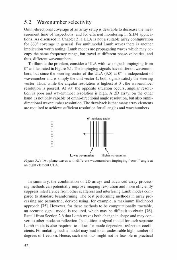
5.2 Wavenumber selectivityOmni-directional coverage of an array setup is desirable to decrease the mea-surement time of inspections, and for efficient monitoring in SHM applica-tions. As discussed in Chapter 3, a ULA is not a suitable array configurationfor 360◦ coverage in general. For multimodal Lamb waves there is anotherimplication worth noting: Lamb modes are propagating waves which may oc-cupy the same frequency range, but travel at different phase-velocities, andthus, different wavenumbers.

To illutrate the problem, consider a ULA with two signals impinging from0◦ as illustrated in Figure 5.1. The impinging signals have different wavenum-bers, but since the steering vector of the ULA (3.5) at 0◦ is independent ofwavenumber and is simply the unit vector 1, both signals satisfy the steeringvector. Thus, while the angular resolution is highest at 0◦, the wavenumberresolution is poorest. At 90◦ the opposite situation occurs, angular resolu-tion is poor and wavenumber resolution is high. A 2D array, on the otherhand, is not only capable of omni-directional angle resolution, but also omni-directional wavenumber resolution. The drawback is that many array elementsare required to achieve sufficient resolution for all angles and wavenumbers.

Figure 5.1: Two plane waves with different wavenumbers impinging from 0◦ angle atan eight element ULA.

In summary, the combination of 2D arrays and advanced array process-ing methods can potentially improve imaging resolution and more efficientlysuppress interference from other scatterers and interfering Lamb modes com-pared to standard beamforming. The best performing methods in array pro-cessing are parametric, derived using, for example, a maximum likelihoodapproach [75]. However, for these methods to be computationally tractable,an accurate signal model is required, which may be difficult to obtain [76].Recall from Section 2.6 that Lamb waves both change in shape and may con-vert to other modes at reflection. In addition, a signal model for each separateLamb mode is also required to allow for mode dependent reflection coeffi-cients. Formulating such a model may lead to an undesirable high number ofdegrees of freedom. Hence, such methods might not be feasible in practical

52

applications. This motivates an evaluation of methods that do not require sucha detailed signal model.

By considering a basic problem, such as, direction of arrival estimation ofa passive source, insight could be gained into properties of Lamb waves thatmight affect the applicability of different methods on the Lamb wave imagingproblem.

5.3 Paper I - Direction of arrival estimationPaper I provides an evaluation of three methods that do not require knowledgeabout the signal waveform, a phase-mode beamformer (PMBF) approach, theMVDR (or Capon) method, and the multiple signal classification (MUSIC)technique. The purpose of the evaluation was to give insight into the propertiesof Lamb waves that might affect the applicability of the MVDR and MUSICapproaches, as well as other methods. The methods were evaluated on bothsimulated and experimental data.

The setup modelled a passive acoustic emission scenario, where an activetransducer emits a multi-cycle sinusoid that propagates in a plate and is re-ceived by a passive UCA. It was assumed that the dispersion characteristics ofthe plate were unknown, as well as the number of propagating modes, makingthe problem a general frequency-wavenumber estimation problem. For eachfrequency, the power of each angle/wavenumber (θ − k) pair was to be esti-mated. The angular power spectrum was then estimated by summation overall wavenumbers for each angle.

In Sections 3.8 and 3.B, the MVDR and MUSIC methods inability of han-dling correlated signals was discussed. In the work presented in Paper I it wasassumed that the impinging signals were uncorrelated, thereby avoiding theneed of preprocessing, such as spatial smoothing, cf. Section 3.8.

The results showed that the MVDR approach and, to some extent, the MU-SIC approach performed significantly better on both simulated and experi-mental data, in terms of higher resolution and lower sidelobes than the phase-mode beamformer, which is basically a standard beamformer. It was furthershown that the MVDR beamformer and the MUSIC approach was less sensi-tive to the "false" grating lobes in the UCA’s array pattern discussed in Sec-tion 3.7. This could allow a less dense, and possibly irregular, array whichwould improve resolution without increasing the number of elements in thearray. This is particularly useful in the presence of multiple modes, since themodes may span a large range of wavenumbers. However, the most significantdrawback of the MVDR and MUSIC approaches when considering imagingare their inability to cope with correlated signal.

53

5.4 Lamb wave imagingThe findings encouraged further investigations on extending the methods fromthe passive array case to an active setup as this would enable imaging. This isthe topic of Papers II and III.

The objective of the plate imaging problem is obviously an accurate repre-sentation of defects in the plate. It can be assumed that the plate is finite andthat the defects have arbitrary shape and are likely to appear at any part ofthe plate. Thus, both near- and far-field coverage using a two dimensional ar-ray is essential. It is also desirable that the proposed method works with bothsingle and multiple transmitter setups. Furthermore, broadband signals are re-quired for high range resolution, and finally, the backscattered signals can beassumed to be highly correlated.

5.4.1 ModelTo provide some insight for the reader into the properties of the setup thatare relevant for imaging, a simplified model is used. Assume that there areR point-scatterers in the plate that scatter incident waves equally in all direc-tions and that no multiple scattering occur between scatterers. Further assumethat the array elements are point-like and perfectly omni-directional in bothtransmission and reception. Hence, assuming also that the output from eachelement is equal to the normal surface displacement, the output from receiv-ing element m, Gm(ω), is the sum of the contributions from all possible modecombinations for all scatterers r for transmitter p as

Gp,m(ω) =R∑

r=1

∑n,n′

1√zr,pzr,m

Rr,n,n′(ω)

·Hn(ω)T (ω)ej(kn(ω)‖zr−zm‖+kn′ (ω)‖zr−zp‖) (5.1)

where zr,p = ‖zr − zp‖ and zr,m = ‖zr − zm‖; zr, zm and zp are the po-sitions of the scatterer, the receiving element, and the transmitting element,respectively. The transfer function Hn(ω) describes the coupling between anexciting stress T (ω) and the resulting normal displacement of mode n. Thepoint scatterers are assumed to have an unknown, frequency and mode depen-dent reflection coefficient Rr,n,n′(ω), where n is the incident mode and n′ thereflected mode. In the case of mode conversion, n and n′ will differ.

5.4.2 Paper II – Single transmitter imagingPaper II concerns the use of a single transmitter – multiple receiver setup forperforming imaging of a plate.

In Secion 3.10 the steered covariance matrix (STCM) was described as analternative approach to frequency domain processing. A modification of the

54

STCM approach has been used to perform focusing in near-field medical ul-trasound imaging in [42, 40, 41]. This approach results in a broadband co-variance matrix focused both in angle and range, thereby requiring one co-variance matrix inversion for each point. However, for broadband dispersiveLamb waves, simply using delays will not align the signals since the frequencycomponents propagate at different phase velocities. A solution to this problemwas proposed in Paper II. By combining the steering operation with dispersioncompensation, cf. Sec 2.A, a focused covariance matrix was estimated for apotential scatterer in each point.

Several snapshots are required for covariance matrix estimation. As dis-cussed in Sec 3.10, averaging over adjacent points may not be a feasible ap-proach for broadband signals. In addition, such averaging does not decorrelatethe signals. Since only one transmitter were available spatial smoothing wasemployed. However, as discussed in Sec. 3.8, spatial smoothing requires aregular array shape to form identical subarrays. Hence, in Paper II a URA wasused, which is a suitable selection allowing 360◦ coverage.

An evaluation of the method was performed on both simulated and experi-mental data. For the experimental evaluation a number of defects were addedto the aluminium plate used for the results in Paper I. The defects were pairs ofdrilled through holes, a 1 cm wide notch, and some artificial pits with depthsof 1 to 3 mm as seen in Figure 5.2. A simplified model of the plate was usedfor the simulation results.

Figure 5.3 shows results from simulated data and Figure 5.4 from experi-mental data. Both the simulated and experimental data show that the MVDRapproach yields much higher resolution and interference suppression than thestandard beamformer. It was further shown in the paper that the proposedmethod performs better in terms of interfering Lamb mode suppression.

Issues related to uncertainties in the array steering vector and correlated sig-nals were discussed. These typically result in underestimation of amplitudes,which could be seen in some of the results.

5.4.3 Paper III - Multiple transmitter imagingA natural extension of the method presented in Paper II, was to use multi-transmitter data. By creating a full multistatic set using all array elements asboth transmitters and receivers, issues related to correlation between sourcesare eliminated. Furthermore, since spatial smoothing is avoided, much smallerarrays could be considered. Simulated and experimental data was used to com-pare the performance of the MVDR approach and the standard beamformer.

Simulations were performed on different array geometries and sizes. A sin-gle reflection of the S0 and A0 modes was simulated and the algorithms abilityto focus on one mode and suppress the other using various array configura-tions was evaluated. The performance of the methods was also evaluated inthe presence of mode conversion.

55

The paper also discusses issues related to focusing of broadband signalswhen using multiple transmitters. It was shown how the different transmitter-receiver pairs creates elliptic shaped focus lines which may cause a singlescatterer to appear spatially smeared between the transmitter snapshots. Fur-thermore, different defects may appear in different snapshots, which increasesthe number of interferers in the estimated covariance matrix. This reduces theefficiency of MVDR beamformer. A method to mitigate these effects is pro-posed and discussed.

Examples of results presented in the paper can be seen in Figure 5.5 forsimulated data and Figure 5.6 for measured data. Again, the MVDR approachclearly outperforms the standard beamformer. In the paper, comparisons of theperformance for different array sizes and configurations show that the MVDRapproach can allow smaller arrays without reduced performance compared toa standard beamformer on a larger array. It was further shown using simu-lated data that 2D arrays in conjunction with the proposed approach yieldsmuch more efficient suppression of interfering Lamb modes compared to thestandard beamformer.

5.5 ConclusionsIt has been shown that a two dimensional array in conjunction with a MVDRbeamformer can significantly improve resolution and interference suppressionin plate imaging. Due to the MVDR approach’s inability to handle correlatedsources, a decorrelating preprocessing step is required for single transmittersetups which reduces the effective aperture size. By contrast, multiple trans-mitter setups do not have this limitation, thereby allowing full aperture utiliza-tion.

56

Figure 5.2: Layout of the aluminum plate with artificial defects. In the results, thearrays were positioned in the center of the plate.

57

x [mm]

y [m

m]

−200 −100 0 100 200

−200

−100

0

100

200

−25

−20

−15

−10

−5

0

x [mm]

y [m

m]

−200 −100 0 100 200

−200

−100

0

100

200

−25

−20

−15

−10

−5

0

Figure 5.3: Results from simulated single transmitter data using standard beamformer(top) and MVDR approach (bottom). White crosses or arrows show which peaks thatare actual defects. The resolution of the MVDR approach is significantly higher. Theinterference shown in the top plot, which is mainly due to interfering modes, is mostlysupressed by the MVDR approach.

58

x [mm]

y [m

m]

−200 −100 0 100 200

−200

−100

0

100

200

−12

−10

−8

−6

−4

−2

0

x [mm]

y [m

m]

−200 −100 0 100 200

−200

−100

0

100

200

−12

−10

−8

−6

−4

−2

0

Figure 5.4: Results from experimental single transmitter data using standard beam-former (top) and MVDR (bottom). White crosses or arrows show which peaks thatare actual holes. The dashed lines show the positions of the pits and the notch, in thecenter right and center left, respectively. Resolution and interference suppression issignificantly better with the MVDR approach.

59

x [mm]

y [m

m]

−200 −100 0 100 200

−200

−100

0

100

200

−20

−15

−10

−5

0

x [mm]

y [m

m]

−200 −100 0 100 200

−200

−100

0

100

200

−20

−15

−10

−5

0

Figure 5.5: Results from simulated multi-transmitter data using standard beamformer(top) and MVDR (bottom). White crosses or arrows show which peaks that are ac-tual defects. Resolution and interference suppression is significantly better with theMVDR approach. The center holes (pair B, cf. 5.2) are not resolved by either of themethods.

60

x [mm]

y [m

m]

−200 −100 0 100 200

−200

−100

0

100

200

−20

−15

−10

−5

0

x [mm]

y [m

m]

−200 −100 0 100 200

−200

−100

0

100

200

−20

−15

−10

−5

0

Figure 5.6: Results from experimental multi-transmitter (3× 3 transmitter array) datausing standard beamformer (top) and MVDR (bottom). White crosses or arrows showwhich peaks that are actual holes. The dashed lines show the positions of the pits andthe notch, in the center right and center left, respectively. Resolution and interferencesuppression is significantly better with the MVDR approach. However, the amplitudesof the holes were underestimated.

61

6. Resonance based methods for theinspection of plate structures

6.1 IntroductionThe previous chapters in this thesis concerned the use of propagating Lambwaves for the inspection and monitoring of structures. That can be regarded asa time domain approach, since range resolution is achieved through temporalseparation.

This chapter concerns the use of resonance techniques for inspection, whichis the topic of Papers IV, V and VI. The work was funded by two EU projects,INCA and NANOSCAN. The participation in these projects involved the de-velopment and evaluation of ultrasonic resonance methods to inspect carbonfiber reinforced plastic (CFRP) panels, and multilayered structures used inaerospace applications. Within the INCA project, special attention was givento weakened bonds. As the name implies, a weakened bond is an adhesivebond where there is contact between the interfaces, but its strength is de-creased. Since the elastic properties of the interface changes very little, thistype of defect is very difficult to detect. By contrast, a complete disbond cre-ates a significant change in the interface and is in many cases detected withoutdifficulty.

An extensive amount of research has focused on the development and evalu-ation of ultrasonic techniques for NDT of adhesive joints. In Chapter 1, Lambwaves were mentioned as one possible technique [5, 6, 7]. Another approachis mechanical impedance analysis (MIA) which has some similarities to theresonance techniques discussed below [77, 78]. Adams and Cawley [79] re-views NDT techniques and defect types that can occur in bonded joints andcomposites.

An object’s natural modes of vibration are a valuable source of informationon the condition of the material. Some approaches, such as resonant ultra-sound spectroscopy (RUS) [80], use techniques to directly measure the reso-nance frequencies of the object. For objects with simple geometries these reso-nance frequency measurements, in conjunction with a physical forward modelof the object, enable estimation of the object’s material properties. However,complex objects are not suitable for this type of estimation due to the difficultyinvolved in creating an accurate model. Hence, a more production oriented ap-plication of this method has been developed based on the detection of changes

63

in the spectrum, so called resonance inspection. Using a large set of good andbad units as training data, units are either passed or failed during the test.

Another approach to utilize an object’s resonance frequencies for testing,is to place on the inspected object a resonant transducer that is acousticallycoupled through a thin layer of couplant. A frequency sweep over a limitedband is performed and an application tailored instrument measures the elec-trical impedance of the probe for a range of frequencies. This means that itis not the resonance spectrum of the structure that is observed, but the res-onance spectrum of the transducer coupled to the structure. The mechanicalload the structure exerts on the transducer will alter the frequency response ofthe transducer. Changes in the position of the resonance frequencies are thenused to detect defects. Since only a limited volume of the inspected object, inthe close vicinity of the transducer, is excited, these inspections are local. Thetechnique is available in some commercial instruments, such as the FokkerBond-Tester.

6.2 Narrowband Ultrasonic SpectroscopyInstead of estimating the properties of certain resonances, such as frequencyor peak-width, the complex valued electrical impedance of a transducer can bemeasured at a single frequency. This approach will be referred to as Narrow-band Ultrasonic Spectroscopy (NBUS) throughout this thesis, to contrast it tothe previously described method used in the Fokker Bond-Tester. As for thatmethod, the transducer is acoustically coupled to the inspected object througha thin layer of couplant, for example, water or oil, as illustrated in Figure 6.1.Defects within the object will result in a change of the load sensed by thetransducer, which can be detected as a change in electrical impedance.

Typically the operator monitors the measurements by observing theimpedance change in the impedance plane between different samples orlocations on the object. These measurements are therefore relative, whichmeans that the impedance measured at the inspected area is compared to theimpedance corresponding to a reference area, preferable defect free. Thetechnique resembles eddy current inspection but a piezoelectric transducer isused instead of a coil.

This technique has been implemented in some commercial instruments, forexample the BondMaster1 series and BondaScope 31002. Setting up an in-spection for impedance measurement involves selecting a transducer and aworking frequency, which is usually set automatically to the resonance fre-quency of the transducer. The most common application of the approach is

1Olymbus NDT2NDT Systems, Inc.

64

Narrowband transducer

Couplant

Layered structure

Z(ω)

Figure 6.1: General NBUS setup (transducer housing and connector are omitted forclarity).

for detecting disbonding in multilayered structures. A disbond is a conditionwhere the adherents are no longer bonded.

6.3 Paper IV – Experimental evaluationIn Paper IV, a model of a narrowband ultrasonic spectroscopy setup is pre-sented along with experimental results from the measurements on aluminium-epoxy structures and CRFPs.

In order to evaluate the basic potential and limitations of the technique,measurements where performed on different defects using various transduc-ers and working frequencies. Experimental results from measurements onsimulated delaminations in aluminium-epoxy structures and CRFPs showedthat transducer and frequency selection are not crucial in those cases. Thiswas not surprising since a delamination completely changes the mechanicalimpedance of the object. However, the amplitude of the impedance changevaried significantly between different transducers and frequencies. Detectionof weakened bonds, on the other hand, proved to be very difficult, and a widerange of transducers and resonance frequencies were tested. This encourageddevelopment of a model which could be used to provide insights and predictthe performance of different setups.

6.4 Paper V & VI – Transducer designPaper V and VI concern transducer design and the identification of relevantproperties of transducers and suitable working frequencies. The basis for thework was a suitable simulation model.

65

The simulations were performed using simplified models of the transducercoupled to the layered structure. These models were based on a one dimen-sional approximation, that is, both the transducer and the structure were as-sumed to be laterally infinite resulting in only thickness motion. A large platestructure can with good accuracy be regarded as semi-infinite. However, thiscan not be assumed in general for a transducer. Therefore, parallel to the one-dimensional model a finite element model was used as a reference, where theeffects of the lateral boundaries of the transducer were taken into account.

The sensitivity, that is, the amplitude of the impedance shift for differenttransducers and frequencies was simulated with respect to two parameters,couplant thickness and the presence of defects. There is no universal model forweakened bonds since the weakness can be caused by a number of problems,such as, contamination between the adherent and the adhesive, and porosity inthe adhesive. The comparison was therefore made by modeling a thin interfacelayer between the adhesive and the adherend. Initially this layer had the sameproperties as the adhesive, but by introducing a small change in its elasticity,the resulting change in impedance of the transducers could be compared. Thisis covered in Paper V.

Paper VI offers an interpretation of the simulation results. Two factors wereidentified that fundamentally determine the performance of the measurement:the standing wave pattern formed in the structure, and the efficiency of theconversion between mechanical and electromechanical energy, the so called,effective electro-mechanical coupling coefficient (EMCC). When the standingwave in the transducer coupled to the structure, matches that of the free res-onating transducer, the sensitivity is maximized. These factors depend on theworking frequency and the transducer design. Transducer design essentiallyinvolves proper selection of the geometry of the piezoelectric element, whichdetermines the resonance frequency of the transducer.

6.5 ConclusionsThe performance of narrowband ultrasonic spectroscopy inspections highlydepends on the transducer type and the selected working frequency. Defects,such as disbonds, are readily detected without careful tuning of the setup.However, weakened bonds are much more difficult to detect. Optimal trans-ducer design and working frequency selection may increase the sensitivity ofthe inspection to certain defects.

66

7. Conclusions

The abundant use of plates in engineered structures and vehicles has stimu-lated the development of techniques for NDT and SHM. The first part of thisthesis considers the use of arrays for Lamb wave inspection and monitoringof plates. Since Lamb waves can propagate over large distances, a large areaof a plate can be covered by a single array.

The results presented in this thesis show that two-dimensional (2D)arrays enable not only angular selectivity, but also wavenumber selectivity.Wavenumber selectivity enables reduction of the interference from otherLamb modes. A review of previous research indicated that most of thepresented work, with few exceptions, were based on standard beamformingmethods. However, for a 2D array setup to have sufficient resolution in alldirections for all wavenumbers, while maintaining low sidelobes, standardbeamforming methods may require a large number of elements, which maybe prohibitive due to practical and economical reasons.

A novel approach for plate imaging using Lamb waves was presented. Ex-tending the use of the MVDR approach, which has previously been applied inother fields of array imaging, to handle dispersive and multi-modal waves re-sulted in a significant improvement in terms of resolution and suppression ofinterference from nearby defects and interfering Lamb modes. Efficient sup-pression of interfering modes allows wider bandwidth of the probing pulses,which improves range resolution and allows more flexibility in the array ele-ment design.

The main drawback of the method, its inability to resolve correlatedsources, can be mitigated either through spatial smoothing, for singletransmitter data, or through the use of multiple transmitters. However, spatialsmoothing reduces the effective aperture size which is a disadvantage forsingle transmitter setups. The use of multiple transmitters eliminates thisissue, thereby enabling full aperture utilization. Hence, multiple transmittersetups are preferred.

A comparison between the MUSIC, MVDR and a standard beamformerapproach on a UCA showed that the MVDR and MUSIC approaches are lesssensitive to, so called, false grating lobes. This enables the use of irregulararrays, which may be not be usable for standard beamformers due to gratinglobes.

The second part of the thesis concerns resonant ultrasound inspection tech-niques of primarily multi-layered plate structures. Simulations and theoretical

67

argumentation showed that the working frequency and the transducer’s reso-nance frequency, which is determined by the type and geometry of its piezo-electric element, greatly affects the attainable sensitivity. Optimal conditionsoccur when the standing wave pattern formed in the transducer and the struc-ture, matches that of the free resonating transducer. This leads to the highestefficiency in the conversion between electrical and elastic energy, which ulti-mately leads to the highest sensitivity.

68

8. Future Work

There are several interesting future directions to explore. A few will be brieflymentioned below.

In this thesis the experimental evaluation of the adaptive imaging approachwas performed on isotropic homogeneous materials only. However, if disper-sion characteristics are available, the method can also be applied to anisotropicor multi-layered plates. Such experimental investigations would be of intereston for example composite structures.

In the presented results, no previous data is reused in the algorithm. Thismay be reasonable when performing a regular inspection. However, for SHMapplications, measurement data may be available from before the actual dam-age occurred. Including such baseline data into the method could improverobustness and sensitivity.

Other signal processing approaches could also be considered. For exam-ple, the iterative adaptive approach (IAA) is a nonparametric weighted leastsquares based method which has been applied to a wide range of problems[81, 82, 83, 84]. Initial results have shown that there are several potential Lambwave applications which would benefit from the approach, such as decompo-sition of Lamb modes, frequency-wavenumber estimation and beamforming.In contrast with the MVDR approach, the IAA method works in both coherentenvironments and can perform well even with only a few snapshots.

An evaluation of model-based approaches would be highly interesting,since such methods typically outperform other methods in scenarios whereaccurate prior information is available. However, the number of unknownsmay be significant, leading to models with a large number of degrees offreedom. Furthermore, the complicated response of the transducer–platecoupling for different modes may require a complicated calibrationprocedure. Although such approach would be of academic interest, its impactin the field are likely limited.

69

9. Swedish Summary

9.1 Oförstörande provningPlåtstrukturer är vanligt förekommande i världen omkring oss. Flygplan, båtaroch cisterner är bara några exempel på fordon eller konstruktioner beståendeav en betydande del platta eller svagt krökta plåtar. Många av dessa tillämp-ningar har höga säkerhetskrav vilket kräver kontinuerlig inspektion. I mångafall kan en okulär besiktning vara tillräcklig, men för kritiska delar av en kon-struktion kan det krävas mer sofistikerade metoder för att bestämma materi-alets inre tillstånd. I de flesta fall finns krav på objektets fortsatta funktionalitetvilket sammanfattar begreppet oförstörande provning (OFP).

Oförstörande provning är inte en teknik, utan ett samlingsnamn för enmängd olika tekniker baserade på olika fysikaliska principer till exempel,magnetism, röntgen eller värmeledning. En teknik som haft stor betydelseför en mängd olika tillämpningar är användandet av högfrekventa elastiskavågor, eller ultraljud. Ultraljudet genereras och tas emot av en sensorkopplad till ett instrument. En vanlig mätprincip, vilken även användsför medicinska tillämpningar, är så kallad pulsekomätning. En kort pulsgenereras som propagerar in i materialet och eventuella förändringar imaterialets egenskaper, naturliga eller skador, resulterar i att en del av pulsenreflekteras. Genom att samla in dessa ekon och söka efter avvikelser, kanman dra slutsatser angående materialets tillstånd. Efterbehandlingen är enviktig del av undersökningen där sofistikerade signalbehandlingsmetoder kananvändas för att ta fram användbar information ur en signal som vid förstaanblick kan se helt slumpmässig ut.

De senaste tjugo åren har en ansenlig mängd forskning fokuserat på vadmånga anser vara nästa stora steg inom området – structural health monitoring(SHM)1. Idén bygger på att sensorer integreras i en konstruktion som därmedkan övervakas kontinuerligt. Genom att tidigt varna för problem kan säker-heten förbättras och kostnader förenade med större haverier minskas.

Denna avhandling behandlar två olika tekniker för inspektion av plåtar. Denförsta delen handlar om propagerande elastiska plåtvågor och den andra omså kallad resonansprovning.

1I brist på vedertaget svenskt begrepp.

71

9.2 Lamb vågorNär ett materials storlek i en eller två riktningar närmar sig våglängden förelastiska vågor i materialet, börjar det bete sig som en vågledare. Vågledareleder den propagerande vågen, vilken under rätt omständigheter kan färdaslånga sträckor utan betydande dämpning. En typ av dessa vågor som upp-kommer i tunna plåtar är så kallade Lamb vågor. Den långa räckvidden fördessa vågor möjliggör undersökning av en större yta av materialet från en fixposition. De senaste årens forskning har lett till ökad förståelse om hur dessavågor beter sig när de propagerar i olika material och i synnerhet hur de reflek-teras. Svårigheten med dessa vågor är att de kan propagera i flera olika moder.Detta innebär att en enda puls som skickas in i plåten kan dela upp sig i fler-talet så kallade moder som färdas med olika hastigheter. Dessutom är dessavågor dispersiva, vilket innebär att pulsen kommer att smetas ut allt eftersomden färdas. Dessa två egenskaper gör analysen av dessa vågor mycket kom-plicerad.

Flertalet publikationer de senaste tio åren har behandlat användandet avgrupper av sensorer, så kallade arrayer. Dessa placeras ut på en mindre yta avplåten. Sensorerna genererar en Lambvåg som sprider sig i plåten. På sammasätt som den ovan beskrivna pulsekotekniken, kommer avvikelser i plåten attresultera i att en del av vågen reflekteras. Dessa reflektioner tas emot av ar-rayens sensorer och kan sedan analyseras i en dator för att rekonstruera enavbildning av plåtens avvikelser. Exempel på sådana avbildningar visas i fig-urerna 5.3–5.6. Tänkbara tillämpningar för dessa arrayer är både tillfälligainspektioner och SHM. I SHM kan ett antal sådana arrayer övervaka en störredel av en plåt.

Den första delen av denna avhandling beskriver utvecklingen av en sig-nalbehandlingsmetod för att rekonstruera dessa avbildningar. Tidigare pub-likationer inom området har varit begränsade till metoder som inte tillvaratarinformationen i de insamlade signalerna på ett effektivt sätt. Den föreslagnametoden kan på ett mer sofistikerat sätt filtrera bort störningar som uppkom-mer av att flera moder propagerar i plåten. Dessutom ger metoden betydligthögre upplösning än vad som åstadkommits tidigare.

9.3 ResonansprovningDen andra delen av denna avhandling berör så kallad resonansprovning.Genom att mäta plåtens så kallade självsvänging, eller resonans, fåsbetydande information om tillståndet inuti plåten. Dessa tekniker har främstanvänts för provning av flerlagerstrukturer och kompositmaterial. Metodernafungerar så att en sensor placeras på materialet som ska undersökas. Sensornär kopplad till ett instrument som får sensorn att vibrera med hjälp av enväxelspänning. Genom att sensorn har kontakt med materialet, kommer en

72

del av den mekaniska rörelsen hos sensorn att fortplanta sig ner i materialetoch reflekteras mot dess undersida. För vissa frekvenser hos växelspänningenkommer resonans att uppstå i både sensorn och materialet tillsammans. Vidförändringar i materialet kommer dessa frekvenser att påverkas. En vanlig typav fel denna metod kan upptäcka är så kallad delamingering. Delamineringinnebär att fogen som håller ihop två lager i en flerlagerstruktur intelängre håller ihop materialen. Denna del av avhandlingen beskriver genomsimuleringar och teoretiska resonemang vilka egenskaper dessa sensorer börha för att maximera känsligheten för olika typer av defekter.

73

10. Acknowledgements

Jag vill börja med att tacka min handledare Tadeusz Stepinski för att jag fåttmöjligheten att utföra detta arbete och som under hela denna tid varit väldigtengagerad i arbetet, vilket har varit ovärderligt.

Ett särskilt stort tack till Tomas Olofsson som ägnat mycket tid till att läsaavhandlingen och manuskripten samt kommit med tydliga förslag till förbät-tringar.

Tack också alla nuvarande och tidigare kollegor på Signaler och system.Det har varit kul att tillbringa denna tid tillsammans med er. Tack för allaintressanta diskussioner.

Jag vill också tacka alla mina vänner utanför jobbet. Hoppas att vi får mertid tillsammans efter det här, trots barn och allt! Särskilt vill jag tacka minakompisar i bandet. Våra rep och inspelningar har varit viktiga avbrott.

Ett stort tack också till mina svärföräldrar Ove och Anita. Jag är tacksamför att ni ställt upp för oss!

Tack mamma, pappa och Sandra för att ni alltid finns där!Sist men inte minst vill jag tacka min familj, Annelie, Elias och Filip. Ni är

det bästa och viktigaste som finns! Jag är så glad att jag har er!

75

Bibliography

[1] C. R. Farrar and K. Worden. An introduction to structural health monitoring.Philosophical Transactions of the Royal Society A: Mathematical, Physical andEngineering Sciences, 365(1851):303–315, 2007.

[2] P. Cawley, M. J. S. Lowe, D. N. Alleyne, B. Pavlakovic, and P. D. Wilcox. Prac-tical long range guided wave testing: Applications to pipes and rail. MaterialsEvaluation, 61(1):66–74, 2003.

[3] J. L. Rose. A baseline and vision of ultrasonic guided wave inspection potential.Journal of Pressure Vessel Technology, 124(3):273–282, 2002.

[4] D. C. Worlton. Experimental confirmation of Lamb waves at megacycle fre-quencies. Journal of Applied Physics, 32(6):967–971, 1961.

[5] S. I. Rokhlin. Lamb wave interaction with lap-shear adhesive joints: Theoryand experiment. The Journal of the Acoustical Society of America, 89(6):2758–2765, 1991.

[6] M. J. S. Lowe and P. Cawley. The applicability of plate wave techniques for theinspection of adhesive and diffusion bonded joints. Journal of NondestructiveEvaluation, 13(4):185–200, 1994.

[7] J. L. Rose, K. M. Rajana, and M. K. T. Hansch. Ultrasonic guided waves forNDE of adhesively bonded structures. The Journal of Adhesion, 50(1):71–82,1995.

[8] E. Lehfeldt and P. Höller. Lamb waves and lamination detection. Ultrasonics,5(4):255–257, 1967.

[9] T. L. Mansfield. Lamb wave inspection of aluminum sheet. Materials Evalua-tion, 33(4):96–100, 1975.

[10] D. N. Alleyne and P. Cawley. Optimization of Lamb wave inspection techniques.NDT & E International, 25(1):11–22, 1992.

[11] D. E. Chimenti and R. W. Martin. Nondestructive evaluation of composite lam-inates by leaky Lamb waves. Ultrasonics, 29(1):13–21, 1991.

[12] N. Guo and P. Cawley. The interaction of Lamb waves with delaminationsin composite laminates. The Journal of the Acoustical Society of America,94(4):2240–2246, 1993.

77

[13] Z. Su, L. Ye, and Y. Lu. Guided Lamb waves for identification of damage incomposite structures: a review. Journal of sound and vibration, 295(3-5):753–780, 2006.

[14] A. Raghavan and C. E. S. Cesnik. Review of guided-wave structural healthmonitoring. Shock and Vibration Digest, 39(2):91 – 114, 2007.

[15] J. L. Rose. Ultrasonic Waves in Solid Media. Cambridge University Press, 1999.

[16] J. D. Achenbach and Y. Xu. Wave motion in an isotropic elastic layer gener-ated by a time-harmonic point load of arbitrary direction. The Journal of theAcoustical Society of America, 106(1):83–90, 1999.

[17] I. I. Nunez, R. K. Ing, C. Negreira, and M. Fink. Transfer and Green func-tions based on modal analysis for lamb waves generation. The Journal of theAcoustical Society of America, 107(5):2370 – 2378, 2000.

[18] T. Demol, P. Blanquet, and C. Delebarre. Lamb waves generation using a flatmulti-element array device. In Proceedings of the 1995 IEEE Ultrasonics Sym-posium, volume 1, pages 791–794, 1995.

[19] R. S. C. Monkhouse, P. D. Wilcox, and P. Cawley. Flexible interdigital PVDFtransducers for the generation of Lamb waves in structures. Ultrasonics,35(7):489–498, 1997.

[20] J. L. Rose, S. P. Pelts, and M. J. Quarry. A comb transducer model for guidedwave NDE. Ultrasonics, 36(1-5):163–169, 1998.

[21] P. D. Wilcox. Omni-directional guided wave transducer arrays for the rapidinspection of large areas of plate structures. IEEE Transactions on Ultrasonics,Ferroelectrics and Frequency Control, 50(6):699 – 709, 2003.

[22] P. D. Wilcox, M. Lowe, and P. Cawley. Omnidirectional guided wave inspectionof large metallic plate structures using an EMAT array. IEEE Transactions onUltrasonics, Ferroelectrics and Frequency Control, 52(4):653–665, 2005.

[23] V. Giurgiutiu. Tuned lamb wave excitation and detection with piezoelectricwafer active sensors for structural health monitoring. Journal of Intelligent Ma-terial Systems and Structures, 16(2):291 – 305, 2005.

[24] D. N. Alleyne and P. Cawley. A two-dimensional fourier transform method forthe measurement of propagating multimode signals. The Journal of the Acous-tical Society of America, 89(3):1159 – 1168, 1991.

[25] M. Niethammer, L. J. Jacobs, J. Qu, and J. Jarzynski. Time-frequency repre-sentations of Lamb waves. The Journal of the Acoustical Society of America,109(5):1841–1847, 2001.

[26] D. N. Alleyne and P. Cawley. The interaction of Lamb waves with defects. IEEETransactions on Ultrasonics, Ferroelectrics and Frequency Control, 39(3):381–397, 1992.

78

[27] Y. Cho and J. L. Rose. A boundary element solution for a mode conversion studyon the edge reflection of Lamb waves. The Journal of the Acoustical Society ofAmerica, 99(4):2097–2109, 1996.

[28] M. J. S. Lowe and O. Diligent. Low-frequency reflection characteristics of theS0 Lamb wave from a rectangular notch in a plate. The Journal of the AcousticalSociety of America, 111(1):64–74, 2002.

[29] M. J. S. Lowe, P. Cawley, J. Y. Kao, and O. Diligent. The low frequency re-flection characteristics of the fundamental antisymmetric Lamb wave a0 from arectangular notch in a plate. The Journal of the Acoustical Society of America,112(6):2612–2622, 2002.

[30] Cho Y. and Rose J. L. An elastodynamic hybrid boundary element study forelastic guided wave interactions with a surface breaking defect. InternationalJournal of Solids and Structures, 37(30):4103 – 4124, 2000.

[31] P. D. Wilcox. A rapid signal processing technique to remove the effect of disper-sion from guided wave signals. IEEE Transaction on Ultrasonics, Ferroelectricsand Frequency Control, 50(4):419–427, 2003.

[32] D. H. Johnson and D. E. Dudgeon. Array signal processing: concepts and tech-niques. Simon & Schuster, 1992.

[33] H. L. Van Trees. Optimum Array Processing (Detection, Estimation, and Mod-ulation Theory, Part IV). Wiley-Interscience, New York, 1 edition, 2002.

[34] J. Capon. High-resolution frequency-wavenumber spectrum analysis. Proceed-ings of the IEEE, 57(8):1408 – 1418, 1969.

[35] P. Stoica and R. L. Moses. Introduction to spectral analysis. Prentice Hall UpperSaddle River, New Jersey, 1997.

[36] B. Widrow, K. Duvall, R. Gooch, and W. Newman. Signal cancellation phenom-ena in adaptive antennas: Causes and cures. IEEE Transactions on Antennas andPropagation, 30(3):469–478, 1982.

[37] H. Hung and M. Kaveh. Focussing matrices for coherent signal-subspaceprocessing. IEEE Transactions on Acoustics, Speech, and Signal Processing,36(8):1272 – 1281, 1988.

[38] T. J. Shan, M. Wax, and T. Kailath. On spatial smoothing for directon-of-arrivalestimation of coherent signals. IEEE Transactions on Acoustics, Speech, andSignal Processing, 33(4):806 – 811, 1985.

[39] K. W. Lo. Adaptive array processing for wide-band active sonars. IEEE Journalof Oceanic Engineering, 29(3):837–846, 2004.

[40] M. Sasso and C. Cohen-Bacrie. Medical ultrasound imaging using the fullyadaptive beamformer. In IEEE International Conference on Acoustics, Speechand Signal Processing, 2005., volume 2, pages 489–492, 2005.

79

[41] J. F. Synnevåg, A. Austeng, and S. Holm. Adaptive beamforming applied tomedical ultrasound imaging. IEEE Transactions on Ultrasonics, Ferroelectricsand Frequency Control, 54(8):1606–1613, 2007.

[42] Z. Wang, J. Li, and R. Wu. Time-delay and time-reversal-based robust Caponbeamformers for ultrasound imaging. IEEE Transactions on Medical Imaging,24(10):1308–1322, 2005.

[43] J. Li, P. Stoica, and Z. Wang. On robust capon beamforming and diagonal load-ing. IEEE Transactions on Signal Processing, 51(7):1702 – 1715, 2003.

[44] J. Li, L. Du, and P. Stoica. Fully automatic computation of diagonal loadinglevels for robust adaptive beamforming. In IEEE International Conference onAcoustics, Speech, and Signal Processing,2008, pages 2325–2328, 2008.

[45] L. Du, J. Li, and P. Stoica. User parameter free approaches to multistatic adap-tive ultrasound imaging. In 2008 IEEE International Symposium on BiomedicalImaging: From Macro to Nano (ISBI ’08), pages 1287 – 1290, 2008.

[46] J. Krolik and D. Swingler. Multiple broad-band source location using steeredcovariance matrices. IEEE Transactions on Acoustics, Speech and Signal Pro-cessing, 37(10):1481 – 1494, 1989.

[47] R. Schmidt. Multiple emitter location and signal parameter estimation. In Pro-ceedings of the RADC Spectrum Estimation Workshop, pages 243–248, 1979.

[48] G. S. Wagner and T. J. Owens. Broadband eigen-analysis for three-componentseismic array data. IEEE Transactions on Signal Processing, 43(7):1738 – 1741,1995.

[49] W. A. K. Deutsch, A. Cheng, and J. D. Achenbach. Self-focusing of Rayleighwaves and Lamb waves with a linear phased array. Research in NondestructiveEvaluation, 9(2):81–95, 1997.

[50] P. D. Wilcox, M. J. S. Lowe, and P. Cawley. Lamb and SH wave transducerarrays for the inspection of large areas of thick plates. In Annual Review ofProgress in QNDE, volume 19A, pages 1049 – 1056, 2000.

[51] P. D. Wilcox. Omni-directional guided wave transducer arrays for the rapidinspection of large areas of plate structures. IEEE Transactions on Ultrasonics,Ferroelectrics and Frequency Control, 50(6):699 – 709, 2003.

[52] P. Fromme, P. D. Wilcox, M. J. S. Lowe, and P. Cawley. On the developmentand testing of a guided ultrasonic wave array for structural integrity monitor-ing. IEEE Transactions on Ultrasonics, Ferroelectrics and Frequency Control,53(4):777 – 785, 2006.

[53] V. Giurgiutiu and J. Bao. Embedded Ultrasonic Structural Radar for the Nonde-structive Evaluation of Thin-Wall Structures. In Proceedings of the 2002 ASMEInternational Mechanical Engineering Congress, pages 17–22, 2002.

80

[54] L. Yu and V. Giurgiutiu. Design, implementation, and comparison of guidedwave phased arrays using embedded piezoelectric wafer active sensors for struc-tural health monitoring. In Proceedings of SPIE, volume 6173, pages 61731M1–61731M12, 2006.

[55] E. Moulin, N. Bourasseau, J. Assaad, and C. Delebarre. Lamb wave beam-steering for integrated health monitoring applications. In Proceedings of SPIE,volume 5046, pages 124–131, 2003.

[56] S. Sundararaman, D. E. Adams, and E. J. Rigas. Structural damage identificationin homogeneous and heterogeneous structures using beamforming. StructuralHealth Monitoring, 4(2):171–190, 2005.

[57] J. Rajagopalan, K. Balasubramaniam, and C. V. Krishnamurthy. A phase re-construction algorithm for Lamb wave based structural health monitoring ofanisotropic multilayered composite plates. The Journal of the Acoustical So-ciety of America, 119(2):872–878, 2006.

[58] F. Yan and J. L. Rose. Guided wave phased array beam steering in compositeplates. In Proceedings of SPIE, volume 6532, pages 65320G.1–65320G.9, 2007.

[59] A. Velichko and P. D. Wilcox. Guided wave arrays for high resolution inspec-tion. The Journal of the Acoustical Society of America, 123(1):186 – 196, 2008.

[60] F. Yan, R. L. Royer jr, and J. L. Rose. Ultrasonic Guided Wave Imaging Tech-niques in Structural Health Monitoring. Journal of Intelligent Material Systemsand Structures, 21(3):377–384, 2010.

[61] M. Fink, C. Prada, F. Wu, and D. Cassereau. Self focusing in inhomogeneousmedia with time reversal acousticmirrors. In Proceedings of the IEEE Ultrason-ics Symposium, pages 681–686, 1989.

[62] D. N. Alleyne, T. P. Pialucha, and P. Cawley. A signal regeneration techniquefor long-range propagation of dispersive lamb waves. Ultrasonics, 31(3):201 –204, 1993.

[63] R. K. Ing and M. Fink. Time recompression of dispersive lamb waves using atime reversal mirror-application to flaw detection in thin plates. In Proceedingsof the IEEE Ultrasonics Symposium, volume 1, pages 659–664, 1996.

[64] R. K. Ing and M. Fink. Self-focusing and time recompression of Lamb wavesusing a time reversal mirror. Ultrasonics, 36(1):179–186, 1998.

[65] D. P. Jansen and D. A. Hutchins. Immersion tomography using Rayleigh andLamb waves. Ultrasonics, 30(4):245–254, 1992.

[66] W. Wright, D. Hutchins, D. Jansen, and D. Schindel. Air-coupled Lamb wavetomography. IEEE Transactions on Ultrasonics, Ferroelectrics, and FrequencyControl, 44(1):53–59, 1997.

81

[67] J. C. P. McKeon and M. K. Hinders. Parallel projection and crosshole Lambwave contact scanning tomography. The Journal of the Acoustical Society ofAmerica, 106(5):2568–2577, 1999.

[68] C. H. Wang, J. T. Rose, and F. K. Chang. A synthetic time-reversal imag-ing method for structural health monitoring. Smart Materials and Structures,13(2):415–423, 2004.

[69] G. Konstantinidis, B. W. Drinkwater, and P. D. Wilcox. The temperature stabil-ity of guided wave structural health monitoring systems. Smart Materials andStructures, 15(4):967–976, 2006.

[70] J. E. Michaels and T. E. Michaels. An integrated strategy for detection andimaging of damage using a spatially distributed array of piezoelectric sensors.In Proc. of SPIE, volume 6532, pages 653203.1–653203.12, 2007.

[71] P. D. Wilcox, A. J. Croxford, J. E. Michaels, Y. Lu, and B. W. Drinkwater. AComparison of Temperature Compensation Methods for Guided Wave Struc-tural Health Monitoring. In Review of Progress in Quantitative NondestructiveEvaluation, volume 975, pages 1453–1460, 2008.

[72] J. E. Michaels, J. S. Hall, and T. E. Michaels. Adaptive imaging of damage fromchanges in guided wave signals recorded from spatially distributed arrays. InProceedings of SPIE, volume 7295, pages 729515–729515–11, 2009.

[73] R. Sicard, J. Goyette, and D. Zellouf. A SAFT algorithm for Lamb wave imagingof isotropic plate-like structures. Ultrasonics, 39(7):487–494, 2002.

[74] R. Sicard, A. Chahbaz, and J. Goyette. Guided Lamb waves and L-SAFT pro-cessing technique for enhanced detection and imaging of corrosion defects inplates with small depth-to wavelength ratio. IEEE Transactions on Ultrasonics,Ferroelectrics and Frequency Control, 51(10):1287–1297, 2004.

[75] H. Krim and M. Viberg. Two decades of array signal processing research: theparametric approach. IEEE Signal processing magazine, 13(4):67–94, 1996.

[76] T. Cicero, P. Cawley, F. Simonetti, and S.I. Rokhlin. Potential and Limitationsof a Deconvolution Approach for Guided Wave Structural Health Monitoring.Structural Health Monitoring, 8(5):381, 2009.

[77] P. Cawley. The impedance method of non-destructive inspection. NDT interna-tional, 17(2):59–65, 1984.

[78] P. Cawley. The sensitivity of the mechanical impedance method of nondestruc-tive testing. NDT international, 20(4):209–215, 1987.

[79] R. D. Adams and P. Cawley. A review of defect types and nondestructive testingtechniques for composites and bonded joints. NDT International, 21(4):208–222, 1988.

82

[80] A. Migliori and J. L. Sarrao. Resonant ultrasound spectroscopy: applicationsto physics, materials measurements, and nondestructive evaluation. Wiley-Interscience, 1997.

[81] J. Ling, T. Yardibi, X. Su, H. He, and J. Li. Enhanced channel estima-tion and symbol detection for high speed multi-input multi-output underwateracoustic communications. The Journal of the Acoustical Society of America,125(5):3067–3078, 2009.

[82] P. Stoica, J. Li, and J. Ling. Missing Data Recovery Via a Nonparametric It-erative Adaptive Approach. IEEE Signal Processing Letters, 16(4):241–244,2009.

[83] T. Yardibi, Jian Li, P. Stoica, Xue M., and A. B. Baggeroer. Source local-ization and sensing: A nonparametric iterative adaptive approach based onweighted least squares. IEEE Transactions onAerospace and Electronic Sys-tems, 46(1):425–443, 2010.

[84] E. Gudmundson, P. Stoica, J. Li, A. Jakobsson, M. D. Rowe, J. A. S. Smith,and J. Ling. Spectral estimation of irregularly sampled exponentially decayingsignals with applications to rf spectroscopy. Journal of Magnetic Resonance,203(1):167 – 176, 2010.

83

�� 0� ��

�/ ��.�12��3��2��4�-�� /�1��2��

��/��/ �� 2��4�-�� /1��2��5��00�� 5� �--��-��-��00��6��7��0 ��2��0��/ �� 8�0��9��7�/ 2��2�� 5�72 ��2�-�� / �� -��/� �� 2��-�2�2�� 3 � ��0��2�� -�� 00�3 �� 2��4�-�� /�1��2��6:;� ��<�-��5��==(5��2�� 7�0-�� 2�/�-�/��2�� >��0��2�� -�� 00��3 �� 2��4�-�� /�1��2��?6@

3 �� -� ��.�0-�� 6--6�-��.��.�.--./ �)&��&,+

��

��

ˇ ˆ - signals and systems, uppsala university · several of the available ndt methods, such as...

Documents