· leonardo pacciani mori [email protected] created date: 12/20/2018 12:50:47 am
TRANSCRIPT

Adaptive metabolic strategies:an (apparently) simple and effective answer to many challenging
problems in ecology and microbiology
The physics of complex systems IV: from Padova to therest of the world and back
Leonardo Pacciani [email protected] 20th, 2018

Introduction: theoretical ecology
Fairly recent discipline (born in 1972 from an article by Robert May)Many open problems
– “Competitive Exclusion Principle” (CEP): the number of competing coexistingspecies in an ecosystem is limited by the number of available resources.
species Sm>p
...
species Sp
...
species S2
species S1
resource Rp
...
resource R1
...
species Sm>p
...
species Sn≤p
...
species S2
species S1
resource Rp
...
resource R1
...
1 of 11

Introduction: theoretical ecologyFairly recent discipline (born in 1972 from an article by Robert May)
Many open problems– “Competitive Exclusion Principle” (CEP): the number of competing coexisting
species in an ecosystem is limited by the number of available resources.
species Sm>p
...
species Sp
...
species S2
species S1
resource Rp
...
resource R1
...
species Sm>p
...
species Sn≤p
...
species S2
species S1
resource Rp
...
resource R1
...
1 of 11

Introduction: theoretical ecologyFairly recent discipline (born in 1972 from an article by Robert May)Many open problems
– “Competitive Exclusion Principle” (CEP): the number of competing coexistingspecies in an ecosystem is limited by the number of available resources.
species Sm>p
...
species Sp
...
species S2
species S1
resource Rp
...
resource R1
...
species Sm>p
...
species Sn≤p
...
species S2
species S1
resource Rp
...
resource R1
...
1 of 11

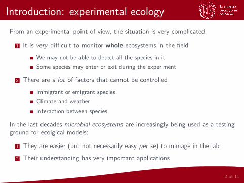
Introduction: experimental ecology
From an experimental point of view, the situation is very complicated:
1 It is very difficult to monitor whole ecosystems in the field
We may not be able to detect all the species in itSome species may enter or exit during the experiment
2 There are a lot of factors that cannot be controlled
Immigrant or emigrant speciesClimate and weatherInteraction between species
In the last decades microbial ecosystems are increasingly being used as a testingground for ecolgical models:
1 They are easier (but not necessarily easy per se) to manage in the lab
2 Their understanding has very important applications
2 of 11

Introduction: experimental ecologyFrom an experimental point of view, the situation is very complicated:
1 It is very difficult to monitor whole ecosystems in the field
We may not be able to detect all the species in itSome species may enter or exit during the experiment
2 There are a lot of factors that cannot be controlled
Immigrant or emigrant speciesClimate and weatherInteraction between species
In the last decades microbial ecosystems are increasingly being used as a testingground for ecolgical models:
1 They are easier (but not necessarily easy per se) to manage in the lab
2 Their understanding has very important applications
2 of 11

The context of our work
“Competitive Exclusion Principle” (CEP): there are many known cases in naturewhere this principle is clearly violated.
1 Bacterial community culture experiments
From Goldford et al. 2018
2 Direct bacterial competition experiments
From Friedman et al. 2017
3 of 11

The context of our work“Competitive Exclusion Principle” (CEP): there are many known cases in naturewhere this principle is clearly violated.
1 Bacterial community culture experiments
From Goldford et al. 2018
2 Direct bacterial competition experiments
From Friedman et al. 2017
3 of 11

The context of our work“Competitive Exclusion Principle” (CEP): there are many known cases in naturewhere this principle is clearly violated.
1 Bacterial community culture experiments
From Goldford et al. 2018
2 Direct bacterial competition experiments
From Friedman et al. 2017
3 of 11

The context of our work“Competitive Exclusion Principle” (CEP): there are many known cases in naturewhere this principle is clearly violated.
1 Bacterial community culture experiments
From Goldford et al. 2018
2 Direct bacterial competition experiments
From Friedman et al. 2017
3 of 11

Modeling ecological competition
Since the ’70s, the main mathematical tool used to model competitiveecosystems has been MacArthur’s consumer-resource model.
species Sm>p
...
species Sp
...
species S2
species S1
resource Rp
...
resource R1
...
ασi
species Sm>p
...
species Sn≤p
...
species S2
species S1
resource Rp
...
resource R1
...
ασi
4 of 11

Modeling ecological competitionSince the ’70s, the main mathematical tool used to model competitiveecosystems has been MacArthur’s consumer-resource model.
species Sm>p
...
species Sp
...
species S2
species S1
resource Rp
...
resource R1
...
ασi
species Sm>p
...
species Sn≤p
...
species S2
species S1
resource Rp
...
resource R1
...
ασi
As it is, the model reproduces the CEP. In order to violate it, very special assumptions orparameter fine-tunings are necessary (Posfai et al. 2017).
4 of 11

Our work
In the literature of consumer-resource models ασi are always considered as fixedparameters that do not change over time.
5 of 11

Our workIn the literature of consumer-resource models ασi are always considered as fixedparameters that do not change over time.
5 of 11

Our workIn the literature of consumer-resource models ασi are always considered as fixedparameters that do not change over time.
Problem B
In many experiments diauxic shifts have been observed (Monod 1949)!
0 2 4 6 8 10 12
0.01
0.05
0.10
0.50
1.00
Time (hours)
Ce
llc
on
ce
ntr
ati
on(g/l)
Growth of Klebsiella oxytoca on glucose and lactose. Data taken from Kompala et al. 1986, figure 11.
5 of 11

Our workIn the literature of consumer-resource models ασi are always considered as fixedparameters that do not change over time.
Our work in one sentenceWe have modified MacArthur’s consumer-resource model so that the metabolicstrategies evolve over time.
5 of 11

Our workIn the literature of consumer-resource models ασi are always considered as fixedparameters that do not change over time.
Our work in one sentenceWe have modified MacArthur’s consumer-resource model so that the metabolicstrategies evolve over time.
How?Adaptive framework: each species changes its metabolic strategies in order toincrease its own growth rate; adaptation velocity is measured by a parameter d .
5 of 11

What we have found
Using adaptive metabolic strategies allows us to explain many experimentallyobserved phenomena, that span from the single species to the whole community!1/4) With one species and two resources, the model reproduces diauxic shifts:
NoticeWe can explain the existence of diauxic shifts with a completely general model,neglecting the particular molecular mechanisms of the species’ metabolism.
6 of 11

What we have foundUsing adaptive metabolic strategies allows us to explain many experimentallyobserved phenomena, that span from the single species to the whole community!
1/4) With one species and two resources, the model reproduces diauxic shifts:
NoticeWe can explain the existence of diauxic shifts with a completely general model,neglecting the particular molecular mechanisms of the species’ metabolism.
6 of 11

What we have foundUsing adaptive metabolic strategies allows us to explain many experimentallyobserved phenomena, that span from the single species to the whole community!1/4) With one species and two resources, the model reproduces diauxic shifts:
NoticeWe can explain the existence of diauxic shifts with a completely general model,neglecting the particular molecular mechanisms of the species’ metabolism.
6 of 11

What we have found
2/4) When multiple species and resources are considered, the model naturallyviolates the Competitive Exclusion Principle:
7 of 11

What we have found
2/4) When multiple species and resources are considered, the model naturallyviolates the Competitive Exclusion Principle:
0 50 100 150 200
101
100
10-1
10-2
10-3
10-4
10-5
10-6
Fixed metabolic strategies
7 of 11

What we have found
2/4) When multiple species and resources are considered, the model naturallyviolates the Competitive Exclusion Principle:
0 50 100 150 200
101
100
10-1
10-2
10-3
10-4
10-5
10-6
Adaptive metabolic strategies
7 of 11

What we have found
3/4) When environmental conditions are variable (i.e. the nutrient supply rateschange in time) using adaptive ασi leads to more stable communities:
8 of 11
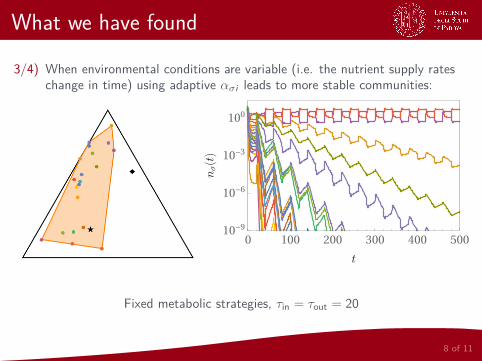
What we have found
3/4) When environmental conditions are variable (i.e. the nutrient supply rateschange in time) using adaptive ασi leads to more stable communities:
0 100 200 300 400 500
100
10-3
10-6
10-9
Fixed metabolic strategies, τin = τout = 20
8 of 11

What we have found
3/4) When environmental conditions are variable (i.e. the nutrient supply rateschange in time) using adaptive ασi leads to more stable communities:
0 100 200 300 400 500
101
100
10-1
10-2
10-3
10-4
10-5
10-6
Adaptive metabolic strategies, τin = τout = 20
8 of 11
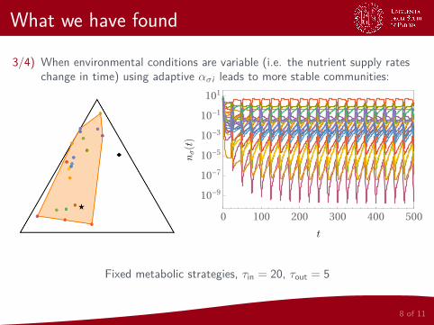
What we have found
3/4) When environmental conditions are variable (i.e. the nutrient supply rateschange in time) using adaptive ασi leads to more stable communities:
0 100 200 300 400 500
101
10-1
10-3
10-5
10-7
10-9
Fixed metabolic strategies, τin = 20, τout = 5
8 of 11

What we have found
3/4) When environmental conditions are variable (i.e. the nutrient supply rateschange in time) using adaptive ασi leads to more stable communities:
0 100 200 300 400 500
101
100
10-1
10-2
10-3
10-4
10-5
10-6
Adaptive metabolic strategies, τin = 20, τout = 5
8 of 11

What we have foundAdaptation velocity d is a crucial element of the model.
4/4) If adaptation is sufficiently slow there can be extinction and theCompetitive Exclusion Principle can be recovered.
20 species, 3 resources
9 of 11

What we have foundAdaptation velocity d is a crucial element of the model.4/4) If adaptation is sufficiently slow there can be extinction and the
Competitive Exclusion Principle can be recovered.
20 species, 3 resources
9 of 11

What we have foundAdaptation velocity d is a crucial element of the model.4/4) If adaptation is sufficiently slow there can be extinction and the
Competitive Exclusion Principle can be recovered.
20 species, 3 resources
9 of 11

Conclusions and future developments
ConclusionsUsing adaptive metabolic strategies in consumer-resource models allows us toexplain lots of different experimentally observed phenomena.
Future developments
Understand more deeply the role of adaptation velocity d : could it be thekey element to predict competition outcome?Design and perform experiments to verify the predictions
10 of 11

Conclusions and future developments
ConclusionsUsing adaptive metabolic strategies in consumer-resource models allows us toexplain lots of different experimentally observed phenomena.
Future developments
Understand more deeply the role of adaptation velocity d : could it be thekey element to predict competition outcome?
Design and perform experiments to verify the predictions
10 of 11

Conclusions and future developments
ConclusionsUsing adaptive metabolic strategies in consumer-resource models allows us toexplain lots of different experimentally observed phenomena.
Future developments
Understand more deeply the role of adaptation velocity d : could it be thekey element to predict competition outcome?Design and perform experiments to verify the predictions
10 of 11

References
Friedman, Jonathan et al. (2017). “Community structure follows simpleassembly rules in microbial microcosms”. In: Nature Ecology and Evolution1.5, pp. 1–7.
Goldford, Joshua E. et al. (2018). “Emergent simplicity in microbial communityassembly”. In: Science 361.6401, pp. 469–474.
Kompala, Dhinakar S. et al. (1986). “Investigation of bacterial growth on mixedsubstrates: Experimental evaluation of cybernetic models”. In: Biotechnologyand Bioengineering 28.7, pp. 1044–1055.
Monod, Jacques (1949). “The Growth of Bacterial Cultures”. In: Annual Reviewof Microbiology 3.1, pp. 371–394.
Posfai, Anna et al. (2017). “Metabolic Trade-Offs Promote Diversity in a ModelEcosystem”. In: Physical Review Letters 118.2, p. 28103.
11 of 11

Backup slides

Details of the model
The equations that define MacArthur’s consumer-resource model are thefollowing:
1 of 3

Details of the modelThe equations that define MacArthur’s consumer-resource model are thefollowing:
1 of 3

Details of the modelThe equations that define MacArthur’s consumer-resource model are thefollowing:
nσ = nσ
( p∑i=1
viασi ri (ci )− δσ
)(1a)
ci = si −m∑σ=1
nσασi ri (ci )− µici (1b)
1 of 3

Details of the modelThe equations that define MacArthur’s consumer-resource model are thefollowing:
nσ = nσ
( p∑i=1
viασi ri (ci )− δσ
)(1a)
ci = si −m∑σ=1
nσασi ri (ci )− µici (1b)
1 of 3
“metabolic strategies”
“resource values”
death rate
resource uptake rate, e.g.ri (ci ) = ci/(Ki + ci )resource supply rate
species’ populations
resources’ concentrations
resource degradation rate

Details of the modelWe can require that ασi evolves so that gσ =
∑pi=1 viασi ri (ci ) is maximized by
means of a simple “gradient ascent” equation:
ασi = 1τσ· ∂gσ∂ασi
= dδσvi ri where 1τσ
= dδσ (2)
Problem B
As it is, eq (2) does not prevent ασi from growing indefinitely!
SolutionWe must introduce some constraint in the resource uptake: the metabolicstrategies ασi must be somehow limited.
2 of 3

Details of the modelOur choice:
p∑i=1
wiασi := Eσ(t) ≤ Qδσ (3)
Final equation (after some work):
ασi = ασidδσ
[vi ri −Θ
( p∑i=1
wiασi −Qδσ
)wi∑p
k=1 w2kασk
p∑j=1
vj rjwjασj
](4)
Attention B
We have also made sure that ασi (t) ≥ 0 ∀t.
3 of 3
“resource costs”

Details of the modelOur choice:
p∑i=1
wiασi := Eσ(t) ≤ Qδσ (3)
Final equation (after some work):
ασi = ασidδσ
[vi ri −Θ
( p∑i=1
wiασi −Qδσ
)wi∑p
k=1 w2kασk
p∑j=1
vj rjwjασj
](4)
Attention B
We have also made sure that ασi (t) ≥ 0 ∀t.
3 of 3
“resource costs”

Details of the modelOur choice:
p∑i=1
wiασi := Eσ(t) ≤ Qδσ (3)
Final equation (after some work):
ασi = ασidδσ
[vi ri −Θ
( p∑i=1
wiασi −Qδσ
)wi∑p
k=1 w2kασk
p∑j=1
vj rjwjασj
](4)
Attention B
We have also made sure that ασi (t) ≥ 0 ∀t.
3 of 3
“resource costs”