© copyright by supriya gupta 2015
TRANSCRIPT


© Copyright by Supriya Gupta 2015
All Rights Reserved

Applying Predictive Analytics to Detect and Diagnose Impending
Problems in Electric Submersible Pumps
A Thesis
Presented to
the Faculty of the Department of Chemical and Biomolecular Engineering
University of Houston
in Partial Fulfillment
of the Requirements for the Degree
Master of Science
in Petroleum Engineering
by
Supriya Gupta
August 2015

Applying Predictive Analytics to Detect and Diagnose Impending
Problems in Electric Submersible Pumps
________________
Supriya Gupta
Approved: ____________________________________
Chair of the Committee
Dr. Michael Nikolaou, Professor
Chemical and Biomolecular Engineering
Committee Members: ____________________________________
Dr. Christine Ehlig-Economides
William C. Miller Endowed Chair Professor
Petroleum Engineering
____________________________________
Dr. Karolos Grigoriadis
David Zimmerman Professor
Associate Director, Aerospace Engineering
Mechanical Engineering
___________________________ ____________________________
Dr. Suresh K. Khator Dr. Thomas K. Holley
Associate Dean Professor and Director
Cullen College of Engineering Petroleum Engineering

v
ACKNOWLEDGEMENTS
This thesis and the underlying research could not have been possible without
significant support from several people during the course of my research. First of all, I
would like to express my deepest gratitude to Dr. Michael Nikolaou for his
encouragement and guidance throughout the course of this research. Through continued
mentorship and support, he helped me build on my interest in data analytics, and carry
out research that can enable practical application of analytics principles in oilfield
production operations.
I am also grateful to Dr. Luigi Saputelli for his invaluable mentorship, brilliant
suggestions and thought provoking feedback throughout the course of my research work.
I deeply value the mentorship of Dr. Cesar Enrique Bravo for highlighting the need for
analytics-driven solutions and sharing his wisdom during several insightful discussions.
I would also like to thank Shyam Panjwani from Professor Nikolaou’s research
group who was instrumental in helping me master analytical techniques for this research.
Furthermore, I am thankful to Vineet Lasrado who volunteered to help me gain access to
the right data for performing analyses and spent significant amount of time in explaining
to me the data-sets and their key characteristics.
I would also like to thank my classmate Shakti Sehra for his support in helping
me master software tools, Anne Sturm at the Petroleum Engineering Department for her
continued support and direction, and my friends and family for their support. Finally, I
would like to thank Dr. Economides and Dr. Grigoriadis, for accepting my request to be
my thesis committee members.

vi
Applying Predictive Analytics to Detect and Diagnose Impending
Problems in Electric Submersible Pumps
An Abstract
of a
Thesis
Presented to
the Faculty of the Department of Chemical and Biomolecular Engineering
University of Houston
in Partial Fulfillment
of the Requirements for the Degree
Master of Science
in Petroleum Engineering
by
Supriya Gupta
August 2015

vii
ABSTRACT
The electrical submersible pump (ESP) is currently the fastest growing artificial-
lift pumping technology. Deployed across 15 to 20 percent of oil-wells worldwide, ESPs
are an efficient and reliable option at high production volumes and greater depths.
However, ESP performance is often observed to decline gradually and reach the point of
service interruption due to factors like high gas volumes, high temperature, and
corrosion. The financial impact of ESP failure is substantial, from both lost production
and replacement costs. Therefore, ESP performance in extensively monitored, and
numerous workflows exist to suggest actions in case of breakdowns. However, such
workflows are reactive in nature, i.e., action is taken after tripping or failure.
Furthermore, given the emerging trend in the E&P industry of using downhole
sensors for real-time surveillance of parameters impacting ESP performance there is an
opportunity for predicting and preventing ESP shutdowns using data analytics. Therefore,
a data-driven analytical framework is proposed to advance towards a proactive approach
to ESP health monitoring based on predictive analytics to detect impending problems,
diagnose their cause, and prescribe preventive action.

viii
TABLE OF CONTENTS
ACKNOWLEDGEMENTS ............................................................. v
ABSTRACT .................................................................................. vii
TABLE OF CONTENTS ............................................................. viii
LIST OF FIGURES .......................................................................... x
LIST OF TABLES .......................................................................... xi
NOMENCLATURE ...................................................................... xii
CHAPTER 1 ..................................................................................... 1
ELECTRICAL SUBMERSIBLE PUMPS ...................................... 1
1.1 Background ........................................................................................ 1
1.2 Challenges with ESP Systems ........................................................... 2
CHAPTER 2 ..................................................................................... 5
STATE OF THE ART ...................................................................... 5
2.1 Monitoring ESP Performance ............................................................ 5
2.2 Troubleshooting ESP Installations .................................................... 6
2.3 Need and Opportunities ..................................................................... 7
CHAPTER 3 ..................................................................................... 9
DATA-DRIVEN ANALYTICS IN OIL AND GAS ....................... 9
3.1 Relevance in Oil and Gas Exploration and Production ..................... 9
3.2 Definition of Analytics ....................................................................10
CHAPTER 4 ................................................................................... 12
ESP ANALYTICS ......................................................................... 12
4.1 Study Objective ................................................................................12
4.2 Study Workflow ...............................................................................12

ix
CHAPTER 5 ................................................................................... 14
ESP ANALYTICS WORKFLOW METHODOLOGY ................ 14
5.1 Prediction of Impending Events ......................................................14
5.1.1 Determination of Decision Variables ............................................................ 14
5.1.2 Application of Principal Component Analysis (PCA) Methodology ........... 18
5.1.3 Model Results ............................................................................................... 23
5.1.4 Pattern Recognition ....................................................................................... 23
5.1.4.1 Pattern Recognition using Scores of Principal components ................ 23
5.1.4.2 Pattern Recognition using Hotelling T-square Statistics ..................... 29
5.2 Diagnosis of Potential Cause ...........................................................31
5.2.1 Contribution Plots ......................................................................................... 31
5.3 Prescription of Preventive Action ........................................................34
5.3.1 Determination of stable operation range ....................................................... 34
5.3.2 Remedial action to correct impending problem ............................................ 36
CHAPTER 6 ................................................................................... 38
CONCLUSION AND RECOMMENDATIONS .......................... 38
6.1 Conclusion ............................................................................................38
6.2 Significance and Recommendations ....................................................39
REFERENCES ............................................................................... 40
APPENDIX .................................................................................... 44
A.1 Principal Component Analysis ........................................................44
A.2 Robust Principal Component Analysis ............................................47

x
LIST OF FIGURES
Figure 1: An electrical submersible pump system [3] ........................................................ 2
Figure 2: Industry Spending on Artificial Lift Technology ................................................ 3
Figure 3: Ammeter Chart Example: Pump off with Gas Interference [9] .......................... 6
Figure 4: Parameters measured by downhole and surface gauges ...................................... 8
Figure 5: ESP Analytics workflow designed for the study ............................................... 13
Figure 6: Stable Operation Zone Parameter Behavior ...................................................... 20
Figure 7: Deviation from normal behavior as observed in parameters ............................. 22
Figure 8: Comparison of Scores of Stable Operation Zone and Trip 1 ............................ 24
Figure 9: Comparison of Scores of Stable Operation Zone and Trip 2 ............................ 26
Figure 10: Comparison of Scores of Stable Operation Zone and Trip 3 .......................... 26
Figure 11: Comparison of Scores of Stable Operation Zone and Trip 4 .......................... 27
Figure 12: Comparison of Scores of Stable Operation Zone and Trip 5 .......................... 27
Figure 13: Hotelling T-square Plot for Stable Operating Zone and various Trips ........... 30
Figure 14: Diagnostic Plot for Trip 1 ................................................................................ 33
Figure 15: Diagnostic Plot for Trip 2 ................................................................................ 33
Figure 16: Prescriptive plot for ESP Heath Performance ................................................. 35
Figure 17: New Hotelling T-square values for the trips after resetting the parameters .... 37
Figure 18: Diagram of Principal Components in 2-D space ............................................. 45

xi
LIST OF TABLES
Table 1: Assumptions and Results from GE Study of ESP failure costs ............................ 4
Table 2: PCA Model Results ............................................................................................ 23

xii
NOMENCLATURE
Variables
H Head generated by the pump, ft
𝜌 Specific gravity of the fluid
Q Pumping Rate, bpd
X Input Matrix
E Residual Matrix
T Scores Matrix
P Loadings Matrix
t Number of time steps or batches
P Number of parameters
R Number of Principal components
D Diagonal Matrix
I Identity Matrix
T2 or D Hotelling T-square statistic
Covariance Matrix
N Count of time steps or batches
𝑥𝑛𝑒𝑤 Prediction dataset for 1 time step or batch [1XP]
𝑐𝑝𝑛 Contribution of parameter p at time step n
𝑐𝑝 Average contribution of parameter p for all time steps in prediction set
𝜒2 Chi-square distribution

xiii
Acronyms
ESP Electrical Submersible Pump
PCA Principal Component Analysis
SCADA Supervisory control and data acquisition
DHM Downhole Measurement
TDH Total Developed Head
PIP Pump Intake Pressure
FBHP Flowing Bottomhole pressure
Superscripts
T Transpose of a Matrix
-1 Inverse of a Matrix
Subscripts
i ith row
new A new batch or time step

1
CHAPTER 1
ELECTRICAL SUBMERSIBLE PUMPS
1.1 Background
Artificial lift techniques are employed when reservoirs do not have enough energy
to naturally produce oil or gas to the surface or at desired economic rates. More than 90%
of producing oil wells require some form of artificial lift [1]. The electrical submersible
pump (ESP) is the fastest growing form of artificial-lift pumping technology [1]. About
15 to 20 percent of almost one million wells worldwide are pumped with some form of
artificial lift employing ESPs [2]. ESPs are often considered very efficient and reliable
for pumping high volumes from deeper depths among all oil field lift systems. They are
adaptable to highly deviated wells and deployed in varied operating environments all
over the world. These pumps have a very broad application range and enable recovery of
hydrocarbon fluids from greater depths at higher temperatures while handling a range of
viscosities, gas-liquid ratios, and solids production.
Figure 1 illustrates a conventional ESP installation system. It primarily consists of
an electric submersible motor, a multistage centrifugal pump, tubing string and protector
section. The ESP runs in the tubing string. The motor is at the lower part of the
installation unit and is a three phase induction motor providing energy to drive the pump.
The protector or seal section connects motor to the pump, prevents well fluids from
entering the motor and equalizes pressures between the motor and the wellbore
A gas separator is situated above the protector and allows well fluids to enter the
centrifugal pump. In addition, it removes free gas from the wellstream. The multistage

2
centrifugal pump, central to the ESP operation, lifts the liquid to the surface. It converts
energy of the electric motor into velocity or kinetic energy and then into pressure energy
of a fluid (head) that is being pumped.
Figure 1: An electrical submersible pump system [3]
1.2 Challenges with ESP Systems
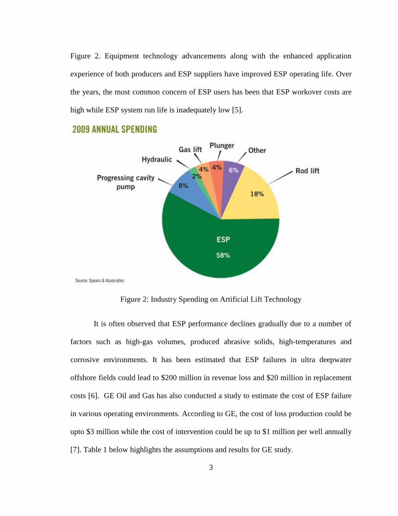
In 2009, Spears & Associates estimated that ESP accounted for 58% of the total
artificial lift market of $5.8 billion [4]. In other words, the industry spends more money
annually on ESPs than for all other forms of artificial lift combined, as illustrated in
3
Figure 2. Equipment technology advancements along with the enhanced application
experience of both producers and ESP suppliers have improved ESP operating life. Over
the years, the most common concern of ESP users has been that ESP workover costs are
high while ESP system run life is inadequately low [5].
Figure 2: Industry Spending on Artificial Lift Technology
It is often observed that ESP performance declines gradually due to a number of
factors such as high-gas volumes, produced abrasive solids, high-temperatures and
corrosive environments. It has been estimated that ESP failures in ultra deepwater
offshore fields could lead to $200 million in revenue loss and $20 million in replacement
costs [6]. GE Oil and Gas has also conducted a study to estimate the cost of ESP failure
in various operating environments. According to GE, the cost of loss production could be
upto $3 million while the cost of intervention could be up to $1 million per well annually
[7]. Table 1 below highlights the assumptions and results for GE study.

4
Table 1: Assumptions and Results from GE Study of ESP failure costs
Lost production Cost
Price of oil barrel $100
Typical production 500 b/d
Water cut 70%
Estimated downtime 2 days
Estimated incidents/year 10
Estimated savings 500 b/d x 20 x 0.3 x $60 = $1.8MM
Intervention Cost
Onshore conventional well $5K to $25K per intervention
Onshore unconventional well $150K to $250K
Offshore well Up to $1MM
Given the high cost of an ESP failure, operators are increasingly using downhole
and surface sensors to monitor ESP performance. Safe operating thresholds for key
parameters are set in ESP so that it proactively stops working if those parameters are
operating beyond its safety limit and a failure is imminent. This is known as a Trip. It is
one step before a failure.
Numerous workflows exist that provide suggestions for actions in case of an ESP
failure. However, such workflows are reactive in nature, i.e., action is taken after a failure
has occurred. Consequently, there is a need and an opportunity to advance from a reactive
approach towards failure situations to a more proactive approach based on predictive
analysis and preventive action by combining reservoir and production engineering
principles with sophisticated mathematical models for predicting ESP trip and failure
events. A proactive approach can be based on monitoring vital statistics related to ESP
operation and performance, thus helping detect impending failures and thereby
optimizing production, reducing intervention costs, and extending the life expectancy of
the ESP.

5
CHAPTER 2
STATE OF THE ART
2.1 Monitoring ESP Performance
As real-time technology gains momentum in the oil industry, more and more wells
are equipped with permanent downhole sensors which offer a wealth of information [8].
Supervisory control and data acquisition (SCADA) systems and data historians offer a lot
of value in terms of reduced operating cost and increased recovery factor [8]. E&P
companies are deploying web-based monitoring platforms for real-time surveillance of
producing assets. Related workflows assist engineers with their daily surveillance
activities for production systems, reservoirs, wells, and fields. This technological
framework is redefining production optimization and reservoir management [1] by
providing numerous capabilities, such as real-time collaboration of asset teams spread
across geographies and enabling faster decision making.
There is a growing trend towards ESPs being fitted with gauges and sensors over the last
decade [8]. These downhole monitoring tools protect the ESP by providing valuable
operational and production data such as pump intake pressure, pump discharge pressure,
bottomhole pressure, motor temperature, current leakage and vibration. A few essential
parameters are continuously monitored and analyzed to assess the health of the ESP
equipment and anticipate impending failure and trip events. This is done to ensure
profitable and safe operations. Furthermore, such data enables production engineers to
perform pressure transient analysis to analyze reservoir performance by monitoring the
key variables during pump shutdowns and startups.

6
2.2 Troubleshooting ESP Installations
ESP system monitoring has evolved over the years and ammeter charts came to be
offered as the earliest and simplest diagnostic solution to minimize downtimes for many
decades. They measure and record the electric current drawn by the ESP motor. The
current is recorded continuously in the function of time on a continuous chart with the
proper scale. Figure 3 is a typical example of Ammeter chart in the scenario of gas
locking. Such behavior is observed when the capacity of the ESP unit is greater than the
inflow to the well and the well produces substantial free gas volumes.
Figure 3: Ammeter Chart Example: Pump off with Gas Interference [9]
The proper interpretation of ammeter charts can provide useful information to
detect and correct minor operational issues [9]. It provides a very one-sided picture of

7
ESP unit’s operations since it relies on only electrical measurements. Electrical failures
are often caused by mechanical or other problems which, over time, develop into a failure
of an electrical nature. The detection of the initial or root failure, therefore, is not an easy
task and requires additional information [9].
The ESP installation works as a system consisting of (1) mechanical, (2)
hydraulic and (3) electrical components [9] and, in order to diagnose and prevent trips or
failure, a dynamic system which can capture multiple parameters affecting an ESP
operation in real-time and provide an end to end solution is necessary.
Nowadays a lot of ESP controllers use microprocessors to provide greatly
improved control and protection of the ESP system’s electric components [10]. They use
several other electrical variables than just the current drawn by the motor which can then
be stored for immediate or future analysis [10]. Many onshore installations use only
ammeter because of the moderate workover costs whereas offshore wells rely on
sophisticated downhole measurements (DHMs) to a great extent [9]. DHMs provide
continuous measurement of crucial downhole parameters such as pump intake pressure
and pump discharge pressure pressure for troubleshooting the system.
2.3 Need and Opportunities
Relevant production data has been growing from kilobytes to terabytes in recent
years, thus becoming “Big Data” [11]. The entire process of gathering, processing, and
analyzing such data is often referred to as analytics [11]. Analytics helps to get
maximum value from production data, identifying patterns that allow for real-time event
detection, failure prevention, production optimization and forecasting, and helping to
reduce the uncertainty in asset management.
8
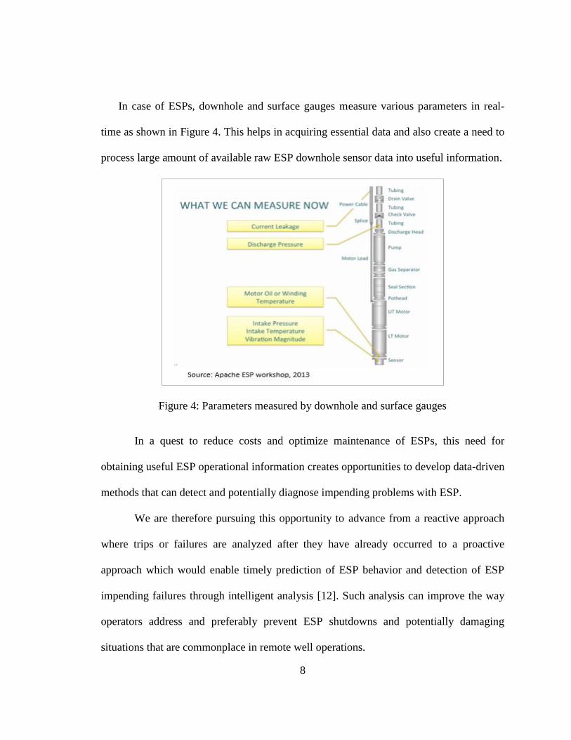
In case of ESPs, downhole and surface gauges measure various parameters in real-
time as shown in Figure 4. This helps in acquiring essential data and also create a need to
process large amount of available raw ESP downhole sensor data into useful information.
Figure 4: Parameters measured by downhole and surface gauges
In a quest to reduce costs and optimize maintenance of ESPs, this need for
obtaining useful ESP operational information creates opportunities to develop data-driven
methods that can detect and potentially diagnose impending problems with ESP.
We are therefore pursuing this opportunity to advance from a reactive approach
where trips or failures are analyzed after they have already occurred to a proactive
approach which would enable timely prediction of ESP behavior and detection of ESP
impending failures through intelligent analysis [12]. Such analysis can improve the way
operators address and preferably prevent ESP shutdowns and potentially damaging
situations that are commonplace in remote well operations.

9
CHAPTER 3
DATA-DRIVEN ANALYTICS IN OIL AND GAS
3.1 Relevance in Oil and Gas Exploration and Production
Historically, E&P Oil and gas industry has used vast quantities of data to
understand subsurface reservoirs and define optimum hydrocarbon evacuation strategies.
Data in the form of seismic surveys, open hole and cased hole logging data, PVT and
core sample analysis, reservoir production and pressure information etc. has been
traditionally used to describe the reservoir and make technical decisions. In the recent
past, improvement in sensors and computation toolkit has shifted the industry’s focus
towards intelligent oilfield technologies that can enable increased real-time surveillance
and analytics to improve oilfield performance. For example, real-time down-hole drilling
data can be paired with production data from nearby wells to help adapt their drilling
strategy, especially in unconventional fields [13]. Such intelligent oilfield capabilities are
provided by a set of tools and techniques known within the industry as analytics [13].
In addition to using analytics techniques developed for oilfield applications,
several analytics commonly used in other industries are also being adapted for application
to oilfield workflows, leading to an increasingly expanding toolkit of robust and effective
solutions for oilfield automation.

10
3.2 Definition of Analytics
Various researchers have provided definitions of analytics as outlined below:
Bravo et al. (2013) have defined analytics as ” a set of techniques and tools
intended for data access, integration, analysis, and visualization, which makes it
possible to identify valuable patterns to improve the decision-making process in a
work environment [11].”
Derrick et al. (2013) define it as “application of ideas from a loose coalition of
technical disciplines, including statistics, artificial intelligence, and information
technology to the discovery and communication of meaningful patterns in data
[14].”
Stone (2007) describes analytics as “investigating pattern-recognition techniques
that find correlations and relationships in large data sets [15].”
In addition to understanding the term analytics, it is especially important to understand
the term “big data”. According to Brule (2013), “big data” has three main features:
volume, velocity, and variety [16]. Therefore, the term “big data” often refers to large,
unstructured datasets with non-standard formats or frequency of data capture. Such
datasets often combine what is called “data in motion” (e.g., real-time data), with “data-
at-rest,” such as configuration and historic data [11].
Analytics can be used to analyze the past, evaluate current performance, and predict
future behavior of a system or process. Bravo et al (2013) have classified analytics into
three categories [11]:
Descriptive analytics: This type of analytics is relies on analysis and visualization
of historic data to obtain insights into a system or process. Typical outcomes from

11
descriptive analytics include dashboards, score cards, business intelligence tools
etc.
Predictive analytics: This type of analytics involves prediction of the future
behavior of a process or system based on analysis of historic data.
Prescriptive analytics: This type of analytics is used to define decisions that
optimize the performance of a system or process based on the models built using
the predictive analytics techniques. Bertolucci (2013) has defined prescriptive
analytics as “technology that goes beyond descriptive and predictive analytics;
prescriptive tools recommend specific courses of action and show the likely
outcome of each decision [17].”

12
CHAPTER 4
ESP ANALYTICS
4.1 Study Objective
The overall objective of this research study is real-time detection and diagnosis of
impending ESP trips or failures. We have adopted the following methodology to achieve
this objective:
Use of historical data to determine and evaluate key operational variables
(decision variables) that affect ESP performance.
Use of a hybrid approach (combination of first principles and empirical statistics)
to develop mathematical models that capture how key variables affect trends and
patterns in the behavior of ESPs. Such trends or patterns can then be associated
with satisfactory operation, impending problems, or existing problems.
Evaluation of effectiveness of the mathematical models in detecting trends and
patterns in available ESP operation data.
Examination of the possibility of using the above models to diagnose potential
causes of detected problems.
Development of an approach to prescribe remedial actions to address the
problems and prevent downtime due to trip or failure.
4.2 Study Workflow
ESP workflow has been designed which integrates different analytical techniques
i.e., predictive analytics, diagnostic analytics and prescriptive analytics in a step by step
manner to provide a complete end to end solution for ESP health monitoring and

13
prevention of trips or failures. In the first step of the workflow, decision variables
significant to ESP operation are used to detect patterns indicating impending events (trips
or failures). In the second step, these parameters are ranked based on their contribution to
the impending event to detect the cause. In the third step, a stable operating range is
determined and a remedial action is suggested to mitigate or prevent the impending event.
Figure 5 illustrates the ESP Analytics workflow designed. The various steps of the
workflow will be described in the following chapters.
Figure 5: ESP Analytics workflow designed for the study

14
CHAPTER 5
ESP ANALYTICS WORKFLOW METHODOLOGY
5.1 Prediction of Impending Events
The first step in the workflow involves prediction of an impending abnormal
event such as a Trip or a Failure which can lead to pump downtime. The intent was to use
real-time data obtained from surface and downhole sensors to build data analytical
models and use the results in a meaningful manner to proactively predict impending
events.
5.1.1 Determination of Decision Variables
It is very important to identify and determine key parameters significant to ESP
performance which can serve as decision variables for input to the analytical model. An
oilfield in the Middle East having well with ESP pumps was chosen for the study. Two
different kinds of data records were obtained:
The first data record contained time series information of different parameters
across surface, wellbore and downhole gauges. The data was being recorded in
real-time at a one minute interval for one well.
The second record contained information on the time when a trip or failure
occurred in that well.
The information from these two records was assimilated to correlate the behavior of
the parameters long before, immediately before and exactly during the trip or failure
event. Five events were analyzed in this study.

15
Twenty-two real time parameters were chosen as decision variables for the model.
These variables are defined below:
1) Flowline Pressure – It is also called the back pressure and is pressure at the
discharge of the tubing from the well.
2) Wellhead Pressure – This is pressure at the wellhead of the producing well.
3) Wellhead Temperature – This is the temperature at the wellhead of the
producing well.
4) Motor Current A, 5) Motor Current B and 6) Motor Current C –The ESP
system contains a three phase induction motor. Downhole sensors measure the
current drawn by the three phases of the motor. Any changes in the pump, the
well, or the electrical system translate into changes in the current drawn by the
ESP motor. Trends in the ESP system’s loading can be detected from these
current changes. Motor damage caused by electrical or mechanical problems can
also be detected from motor current. Changes in produced fluid properties can
also be traced by monitoring motor current [9].
7) Pump Intake Pressure -This parameter indicates the flowing pressure in the well
at the level of the ESP pump’s suction. The PIP helps to detect whether free gas
enters the pump or not [9]. It is also strongly related to the well’s FBHP (flowing
bottomhole pressure) and its inflow rate; greater PIPs meaning lower liquid rates
[9]. Because of all these factors, PIP can provide a reliable way to control the
operation of the ESP system. Changes in PIP indicate changes in pump
performance, well inflow, or installation integrity [9].

16
8) Pump Discharge Pressure - It is a measure of the discharge pressure of the
pump. This reading and the pump intake pressure provide a measurement of the
total developed head (TDH) of the pump. Comparison of this value to the design
TDH enables monitoring of hydraulic performance of the pump.
9) Intake Temperature - This measurement provides the temperature of the intake
fluid into the pump. It increases as warmer reservoir fluids flow into the wellbore.
10) Leakage Current – This measurement is the current leakage from the ESP cable
due to earth fault.
11) Motor Temperature - Motor temperature is the measured temperature of the
motor windings or that of the motor oil [9]. If used in system control, measured
temperature must not be allowed to rise significantly above the motor’s rated
temperature.
12) System Vibration -System vibration indicate the onset of problems which may
later lead to more severe mechanical or electrical problems.
13) Water Cut – It is a measure of the ratio of water produced to the amount of total
liquids produced in the well.
14) Free Gas Intake - It is a measure of the gas produced in the wellbore that enters
into the pump. Free gas in the ESP pump rapidly ruins the pump’s efficiency and
increased gas volumes may cause fluctuations of pump output causing surges in
well production.
15) Total Liquid Flowrate – It is a measure of the total liquids being produced in the
well. It allows the determination of the pump’s operating point on the
performance curve. It is the first indicator of downhole problems such as

17
equipment wear, leaks, etc. Changing well inflow can easily be detected from the
trend of liquid rate [9].
16) System efficiency – This is the ratio of the power exerted by the pump to lift a
given amount of liquid against the operating head (Phydr) and the mechanical
power required to drive the pump (BHP) [9]. Phydr is calculated using the
equation
𝑃ℎ𝑦𝑑𝑟 = 7.368 ∗ 10−6𝐻𝑞𝜌, (1)
where H is head generated by the pump in ft, q is the pumping rate in bpd and 𝜌
specific gravity of the fluid.
17) Pump Fluid Density – This is the density of the fluid entering the centrifugal
pump. The centrifugal pump imparts a high rotational velocity on the fluid
entering its impeller but the amount of kinetic energy passed on to the fluid
greatly depends on the given fluid’s density. Liquid, being denser than gas,
receives a great amount of kinetic energy that, after conversion in the pump stage,
increases the pressure whereas gas cannot produce the same amount of pressure
increase [9]. Due to this reason, centrifugal pumps should always be fed by gas-
free, single-phase liquid to ensure reliable operation [9].
18) Pump Head- The pressure rise associated with the liquid passing through all the
stages of the pump made up of rotating impeller and stationary diffuser in series
[9]. Pump head is a function of the diving frequency, flow rate, number of pump
stages, fluid gravity and pump efficiency [9].

18
19) Total Pump Head- This corresponds to the total dynamic head. It is the total
equivalent height to which the fluid is pumped and considering friction losses in
the wellbore.
20) P across Pump – This is the difference of the discharge pressure of the pump
and the intake pressure of the pump. It represents the increase in the operating
pressure of the ESP.
21) P across Choke – This is the difference between wellhead pressure and the
flowline pressure. It helps to estimate the value of the back pressure
22) P ESP to Wellhead – This is the difference of the discharge pressure of the
pump and the wellhead pressure.
The data for these parameters was obtained at a frequency of one minute for a two
year time period for one well. This time period saw several failure and trip events. The
reason behind choosing a large number of variables (22) some of which are inter-
dependent was to be able to capture behavior of all kinds of different attributes which
could essentially lead to different failures.
5.1.2 Application of Principal Component Analysis (PCA) Methodology
After the decision variables were determined, data-driven techniques employing
multi-variate statistics were applied to build models to detect and potentially diagnose
impending problems with ESP operation.
Since we are trying to analyze twenty two parameters in real time with a
frequency of one minute, it is imperative to use a statistical technique which can reduce
the dimensionality in space and provide vectors which are a combination of more than

19
one of the decision variables. This enables us to observe the behavior of the reduced
variables and draw patterns to link to anomalies. In addition, absence of an output
dependent variable which is a consequence of the input parameters eliminates the
possibility of using any regression techniques.
Principal Component Analysis (PCA) methodology is a dimensionality reduction
data driven methodology explained in Appendix A.1. It was chosen for modeling real
time decision variables to identify patterns in the data. It is a statistical technique that
uses an orthogonal transformation to convert a set of observations of possibly correlated
or dependent variables into a set of linearly uncorrelated variables which are called
Principal Components [18]. The covariance among each pair of principal components is
zero. In this manner, PCA removes all the dependencies within the variables. The number
of principal components is less than or equal to the number of original variables [19].
Unfortunately in classical PCA, both the classical variance (which is being
maximized) and the classical covariance matrix (which is being decomposed) are very
sensitive to anomalous observations [19]. Therefore as a consequence, the first
components are often attracted toward outlying points and may not capture the variation
of the regular observations [19]. This can lead to the conclusion that data reduction based
on classical PCA becomes unreliable if outliers are present in the data [19].
In our analysis, since we are obtaining real time downhole data there is a very
high probability of encountering outliers as at times the sensors do not function properly
or are recording erroneous data. So, Robust PCA [19] technique as explained in
Appendix A.2 was adopted for modeling purposes to remove outliers and use the

20
meaningful data readings as an input feed to the model. The model was constructed using
PLS Eigenvector Toolbox integrated within Matlab.
The PCA model used in the study follows a three step process.
Feed Training Dataset
From the real time data, a stable time period was identified when no trip or
failure event was observed and all the 22 parameters were operating at a stable
value Figure 6 is an example plot of four such variables operating at a stable value
for the entire time range. This data set matrix of t time steps or batches and p
parameters (22) was chosen as the X matrix and normalized and fed into the PCA
model.
Figure 6: Stable Operation Zone Parameter Behavior
21
Run Robust PCA Model
Using the dataset chosen in the earlier step, Robust PCA model was run to
resist 25% of the outliers. Corresponding T, P and E matrices were obtained as a
result of the model. T matrix is the scores matrix [tXR], which is a resultant
matrix of the value of Principal components (R) at very time step(t). P matrix is
the loadings matrix [pXR] which represents the correlations between variables
and the principal components. Optimized number of principal components were
selected so that the total number of principal components captured majority of the
variance in data and any further increase in the number of principal components
did not capture significantly increase the variance captured. First principal
component explains as much as possible variance in the data set and the second
principal component explains the next possible variance and the last principal
component explains the lowest variance. The T matrix obtained for the stable
operating zone was obtained and used for comparison at later stages. The model is
created with the loadings matrix P and the residual matrix E and can be used for
any future analysis.
Feed Prediction Dataset
From the real time data sets, we identified windows of time periods when
deviations from stable behavior were observed. These transition zones where the
abnormal behavior started until the time when a trip or failure was observed were
captured. Behavior of only four parameters during the transition zones for three
different trip prediction sets are shown in three red boxes in Figure 7. These
matrices were fed as independent Prediction X matrices, each of t time steps by p

22
variables (22) into the model created in the preceding step. For each of the
prediction sets, the t time period starts at the point when a deviation from normal
trend is seen to the time when the trip or failure eventually occurs. The length of
the time period t may vary for each of the trip or failure events depending on how
long the deviation from normal behavior was observed. The model with the P and
E matrix is rerun for each of these new X matrices. A new T matrix for each
prediction data set is obtained and compared against the stable T matrix recorded
in the preceding step. This comparison is explained in the section 5.1.4.
Figure 7: Deviation from normal behavior as observed in parameters
23
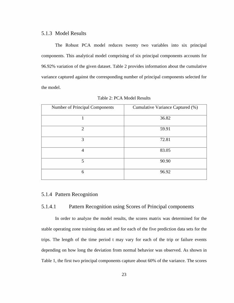
5.1.3 Model Results
The Robust PCA model reduces twenty two variables into six principal
components. This analytical model comprising of six principal components accounts for
96.92% variation of the given dataset. Table 2 provides information about the cumulative
variance captured against the corresponding number of principal components selected for
the model.
Table 2: PCA Model Results
Number of Principal Components Cumulative Variance Captured (%)
1 36.82
2 59.91
3 72.81
4 83.05
5 90.90
6 96.92
5.1.4 Pattern Recognition
5.1.4.1 Pattern Recognition using Scores of Principal components
In order to analyze the model results, the scores matrix was determined for the
stable operating zone training data set and for each of the five prediction data sets for the
trips. The length of the time period t may vary for each of the trip or failure events
depending on how long the deviation from normal behavior was observed. As shown in
Table 1, the first two principal components capture about 60% of the variance. The scores
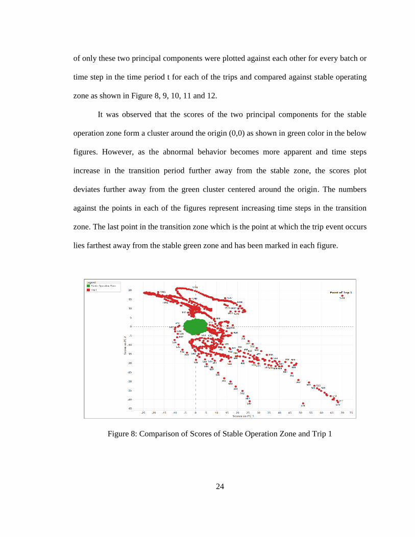
24
of only these two principal components were plotted against each other for every batch or
time step in the time period t for each of the trips and compared against stable operating
zone as shown in Figure 8, 9, 10, 11 and 12.
It was observed that the scores of the two principal components for the stable
operation zone form a cluster around the origin (0,0) as shown in green color in the below
figures. However, as the abnormal behavior becomes more apparent and time steps
increase in the transition period further away from the stable zone, the scores plot
deviates further away from the green cluster centered around the origin. The numbers
against the points in each of the figures represent increasing time steps in the transition
zone. The last point in the transition zone which is the point at which the trip event occurs
lies farthest away from the stable green zone and has been marked in each figure.
Figure 8: Comparison of Scores of Stable Operation Zone and Trip 1

25
It is observed that the transition zone spirals around the green zone in Figure 8.
This pattern can be justified and correlated with the actual scenario leading to the trip. In
the first half of the transition zone, there was an increase in motor temperature because of
underutilization of the pump leading to abnormal functioning of ESP. During this time
period, as time steps increase, the scores shown in red deviate further away from the
stable values within the green zone. This behavior continued until 580th minute.
However, to resolve the issue, the production engineer increased the choke flow rate to
increase the drawdown. This behavior is captured by the pattern depicted between 581st
and 682nd minute where the scores start moving towards the stable range due to the
mitigation steps being taken on the field. However, during the drawdown the wellbore
pressure while decreasing reached below the bubble point leading to production of gas in
the ESP pump. This behavior is shown starting 842nd minute when the scores again start
deviating from the green zone. The increased production of gas lead the ESP to trip at
1518th minute. In this manner, the mathematical results are correlated to the actual
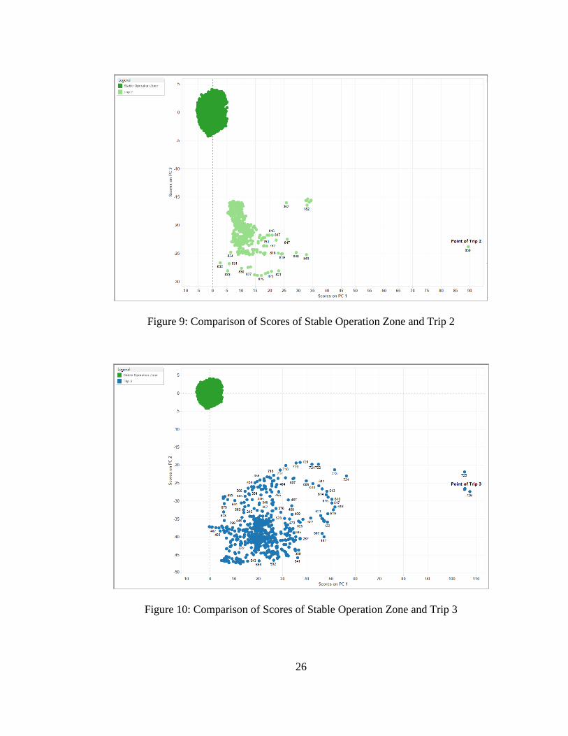
physics of the ESP trip event.
In another example, the transition from the normal behavior was observed for 850
minutes until it tripped in the scenario depicted in Figure 9 and no steps were adopted to
resolve the issue. Today there is no mechanism to record and visualize this abnormal
behavior. Having a dashboard representation of ESP operation using PCA model can help
the engineers visualize and analyze the health of ESP under observation.
26
Figure 9: Comparison of Scores of Stable Operation Zone and Trip 2
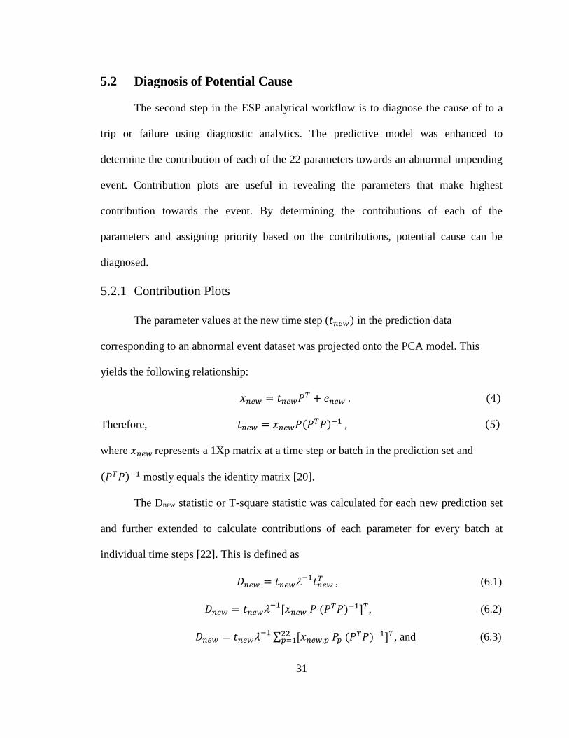
Figure 10: Comparison of Scores of Stable Operation Zone and Trip 3

27
Figure 11: Comparison of Scores of Stable Operation Zone and Trip 4
Figure 12: Comparison of Scores of Stable Operation Zone and Trip 5

28
These patterns help distinguish between stable operation conditions and
impending abnormal events in ESPs. This pattern recognition approach can help us
proactively monitor and predict trips and failures in advance. The trip happens at 1518
time step in Figure 9. As the frequency of time steps is in minutes, therefore the trip
happened at 1518th minute from start of the abnormal transition region. As this is a real
scenario from an oilfield, it can be inferred that the ESP was behaving abnormally for
more than 24 hours before it actually tripped. Had this mechanism of identifying patterns
using PCA Modeling been in place, there would have been ample time for preventive
action that could mitigate or altogether avoid each problem.
This methodology can be extended to a real-time monitoring platform to observe
health of any ESP. The Robust PCA model can be initially trained using stable time
period data for the different parameters. The first two principal components can be used
to get the green stable zone in the plot of scores of principal component 1 and principal
component 2. Once, the model is trained and we have obtained the P and E matrix, the
data for the various parameters obtained from the sensors every minute can be
assimilated and fed as prediction data into the model to obtain the new scores of the first
two principal components at that time step. This can be continuously fed for every time
step and the results can be obtained. As long as ESP is operating smoothly, the point will
lie within the green zone. Otherwise, if with increasing time steps, it is observed that the
points move farther away from the stable zone cluster, it indicates that the ESP is
functioning abnormally and approaching towards a trip or a failure.

29
5.1.4.2 Pattern Recognition using Hotelling T-square Statistics
In the general form the PCA Model, 𝑋 = 𝑇𝑃𝑇 + 𝐸, 𝑇𝑃𝑇 represents the
systematic part of the process variation described by the model and the residual matrix 𝐸
contains the non-systematic part not described by the model [20]. T is columnwise
orthogonal and P is columnwise orthonormal, i.e., 𝑇𝑇𝑇 = 𝐷 and 𝑃𝑇𝑃 = 𝐼, where D is a
diagonal matrix and I is the identity matrix [20].
The Hotelling T-square statistic represent a measure of the variation in each
sample in the model. It indicates how far each sample is from the center (scores = 0) of
the model [21].
𝐻𝑜𝑡𝑒𝑙𝑙𝑖𝑛𝑔 𝑇2𝑖 = 𝑡𝑖−1𝑡𝑖
𝑇, (2)
where ti refers to the ith row of TR, the t X R matrix of scores for each new batch or time
step in the model; is the covariance matrix of stable operation zone T [20] and is a
diagonal matrix containing the eigenvalues 1 through 𝑅 corresponding to R principal
components in the model represented as
−1=
𝑇𝑇𝑇
(𝑁−1)−1 , (3)
where N represents the count of time steps or batches obtained for the stable operation
zone
Hotelling T-square distribution statistic was calculated at every time step in the
stable operation zone and the various transition zones leading the trips. This statistic was
plotted against time on a semi-log plot as shown in Figure 13. It was observed that this
statistic monitored over time stays within the chi-square limit for stable operation and

30
exceeds the limit during unstable (transient) ESP operation, long before an ESP trips or
fails. The actual value of this statistic during the transition period leading to a trip or
failure shows an increase of more than two orders of magnitude compared to its normal
value. The statistic successfully identified all impending trips or failures a few hours
before they actually occurred as shown in Figure 13.
Figure 13: Hotelling T-square Plot for Stable Operating Zone and various Trips
By proactively monitoring the Scores Plot and the Hotelling T-square Plot in real-
time, an impending event can be predicted much in advance. However, predicting an
impending event is not a complete solution. As part of this study, models to diagnose the
cause and prevent an ESP from failing were also established.
31
5.2 Diagnosis of Potential Cause
The second step in the ESP analytical workflow is to diagnose the cause of to a
trip or failure using diagnostic analytics. The predictive model was enhanced to
determine the contribution of each of the 22 parameters towards an abnormal impending
event. Contribution plots are useful in revealing the parameters that make highest
contribution towards the event. By determining the contributions of each of the
parameters and assigning priority based on the contributions, potential cause can be
diagnosed.
5.2.1 Contribution Plots
The parameter values at the new time step (𝑡𝑛𝑒𝑤) in the prediction data
corresponding to an abnormal event dataset was projected onto the PCA model. This
yields the following relationship:
𝑥𝑛𝑒𝑤 = 𝑡𝑛𝑒𝑤𝑃𝑇 + 𝑒𝑛𝑒𝑤 . (4)
Therefore, 𝑡𝑛𝑒𝑤 = 𝑥𝑛𝑒𝑤𝑃(𝑃𝑇𝑃)−1 , (5)
where 𝑥𝑛𝑒𝑤 represents a 1Xp matrix at a time step or batch in the prediction set and
(𝑃𝑇𝑃)−1 mostly equals the identity matrix [20].
The Dnew statistic or T-square statistic was calculated for each new prediction set
and further extended to calculate contributions of each parameter for every batch at
individual time steps [22]. This is defined as
𝐷𝑛𝑒𝑤 = 𝑡𝑛𝑒𝑤−1𝑡𝑛𝑒𝑤
𝑇 , (6.1)
𝐷𝑛𝑒𝑤 = 𝑡𝑛𝑒𝑤−1[𝑥𝑛𝑒𝑤 𝑃 (𝑃𝑇𝑃)−1]𝑇, (6.2)
𝐷𝑛𝑒𝑤 = 𝑡𝑛𝑒𝑤−1 ∑ [𝑥𝑛𝑒𝑤,𝑝 𝑃𝑝 (𝑃𝑇𝑃)−1]𝑇22
𝑝=1 , and (6.3)
32
𝐷𝑛𝑒𝑤 = ∑ 𝑡𝑛𝑒𝑤−1[𝑥𝑛𝑒𝑤,𝑝 𝑃𝑝 (𝑃𝑇𝑃)−1]𝑇22
𝑝=1 . (6.4)
Therefore, the contribution of each parameter 𝑥𝑛𝑒𝑤,𝑗 of a new batch 𝑥𝑛𝑒𝑤 to the D
statistic equals 𝑐𝑝= 𝑡𝑛𝑒𝑤−1[𝑥𝑛𝑒𝑤,𝑗 𝑃𝑝 (𝑃𝑇𝑃)−1]𝑇 [20] where 𝑡𝑛𝑒𝑤 is a matrix of 1X R,
−1 is a matrix of RXR, 𝑥𝑛𝑒𝑤,𝑗 is a matrix of 1X1, 𝑃𝑝 is a matrix of 1XR and P is a matrix
of PXR.
Average contribution of each parameter for the prediction set having t time steps is
𝐶𝑝 = ∑𝑐𝑝𝑛
𝑡
𝑡𝑡=1 . (7)
The contributions can help in deciding the ranking of parameters. Higher the
value of the contribution, higher is the rank. The ranking chart can be used to determine
the parameter causing the impending failure or trip. Diagnostic plots for two Trip
scenarios are shown in Figure 14 and Figure 15. The parameters in these plots are
arranged in decreasing order of their contribution from left to right. Motor Temperature
mainly lead to the abnormal behavior in Trip 1. The ranking of the parameters using this
methodology are in agreement with what was observe during this trip as explained in
Section 5.1.4.1 with regard to Figure 7. Motor temperature can increase due to production
of gas in the pump, presence of abrasive solids or underutilization of the pump. In this
scenario, as the choke was increased, the scores started to adjust snd move towards the
stable zone. However, if by increasing the choke, the scores would have not moved
towards stable zone as was observed in Figure 7, it would indicate that the correct action
is not being taken to solve the problem. It could also mean that there is skin and
increasing the choke is not the solution. It would perhaps require a stimulation job to

33
resolve the problem. In this manner, combination of ESP health monitoring using pattern
recognition and contribution charts can help troubleshoot and fix the problems.
Figure 14: Diagnostic Plot for Trip 1
System Vibration mainly influenced the abnormal behavior in Trip 2. Vibrations
indicate onset of potential severe mechanical or electrical problems.
Figure 15: Diagnostic Plot for Trip 2
0.000
0.2000.4000.600
0.8001.0001.200
1.400
Co
ntr
ibu
tio
n
Parameters
Diagnostic Plot for Trip 1
0.000.200.400.600.801.001.20
Co
ntr
ibu
ton
Parameters
Diagnostic Plot for Trip 2

34
These contribution charts can be extended to a real-time monitoring platform and
can contribute towards diagnosing the cause behind an abnormal behavior in real-time.
5.3 Prescription of Preventive Action
The third step in the workflow is application of Prescriptive analytics to suggest
remedial steps to correct the abnormal behavior and avoid trips or failures.
5.3.1 Determination of stable operation range
Dnew statistic definition can be further extended as [23]
𝐷𝑛𝑒𝑤 = 𝑡𝑛𝑒𝑤−1𝑡𝑛𝑒𝑤
𝑇 ~ 𝑅(𝐼2−1)
𝐼(𝐼−𝑅)𝐹(𝑅, 𝐼 − 𝑅, 𝛼). (8)
The D-statistic divided by some constant, follows an F-distribution with R and I-
R degrees of freedom. 𝛼 represents the boundary and is equivalent to the value at which
the cdf of the probability distribution is equal to 0.95.
We used the above equation to calculate the stable operating range for each
parameter by setting an inequality as
𝑡𝑛𝑒𝑤−1𝑡𝑛𝑒𝑤
𝑇 ≦ 𝑅(𝐼2−1)
𝐼(𝐼−𝑅)𝐹(𝑅, 𝐼 − 𝑅, 𝛼). (9.1)
On substituting the value of 𝑡𝑛𝑒𝑤 from equation (5),
𝑥𝑛𝑒𝑤𝑃−1𝑃𝑇𝑥𝑛𝑒𝑤 𝑇 ≦
𝑅(𝐼2−1)
𝐼(𝐼−𝑅)𝐹(𝑅, 𝐼 − 𝑅, 𝛼), (9.2)
where 𝑥𝑛𝑒𝑤 is a 1XP matrix. In order to determine the minimum and maximum stable
operating values and set an operating range for each parameter, we solve the above
quadratic inequality individually for each parameter 𝑥𝑛𝑒𝑤,𝑝 and setting the stable

35
operating values used in the training dataset for the other P-1 parameters within 𝑥𝑛𝑒𝑤
matrix.
Figure 16: Prescriptive plot for ESP Heath Performance
The green bars in Figure 16 represent the stable operating range for each of the 22
parameters. Since there is significant difference between magnitudes of various
parameters, the operating value is expressed in percentage. The line graphs represent the
reading of the various parameters at the time of two separate trip events, Trip 1 and Trip
2.
0
50
100
150
200
250
Op
erat
ing
Val
ue
(%)
Decision Variables
Prescriptive Plot for ESP Health Performance
Stable Zone Trip 1 Trip 2

36
This plot is useful to distinguish between parameters operating within the stable range
and those operating outside their stable ranges and show how far are some of the
parameters operating outside their stable ranges in real time for every time step.
Controllable parameters such as choke and motor current can be reset such that all the
parameters get adjusted to lie within the stable green bands. This plot is significant in
enabling effective decision making and can also be extended to monitor the behavior of
parameters in real-time operations.
5.3.2 Remedial action to correct impending problem
By resetting those parameters which are operating outside the stable green bands
to a value inside the stable ranges, it is possible to correct the abnormal behavior and
ensure that the ESP operates smoothly again.
The F-distribution has relationship with chi-square distribution [24]. Therefore,
the above relationship can be represented as
𝑅(𝐼2−1)
𝐼(𝐼−𝑅)𝐹(𝑅, 𝐼 − 𝑅, 𝛼) ~𝜒2. (10)
Once the parameters are reset to ensure that all parameters are operating inside
stable bands, this batch is fed as prediction dataset into the model again. The new
Hotelling T-square value obtained for this batch was observed to be within the stable
operating zone. On substituting Equation (9.1) in Equation (10), we get
𝑇𝑖,𝑟𝑒𝑐𝑎𝑙𝑐𝑢𝑙𝑎𝑡𝑒𝑑2 = 𝑡𝑖,𝑟𝑒𝑐𝑎𝑙𝑐𝑢𝑙𝑎𝑡𝑒𝑑
−1𝑡𝑖,𝑟𝑒𝑐𝑎𝑙𝑐𝑢𝑙𝑎𝑡𝑒𝑑𝑇 ≦ 𝜒2. (11)
Hence, the recalculated value of Hotelling T-square statistic which was earlier
more than two orders of magnitude is now less than 𝜒2. It was observed that this statistic
now stayed within the 95% confidence limit for the prediction data batch and did not
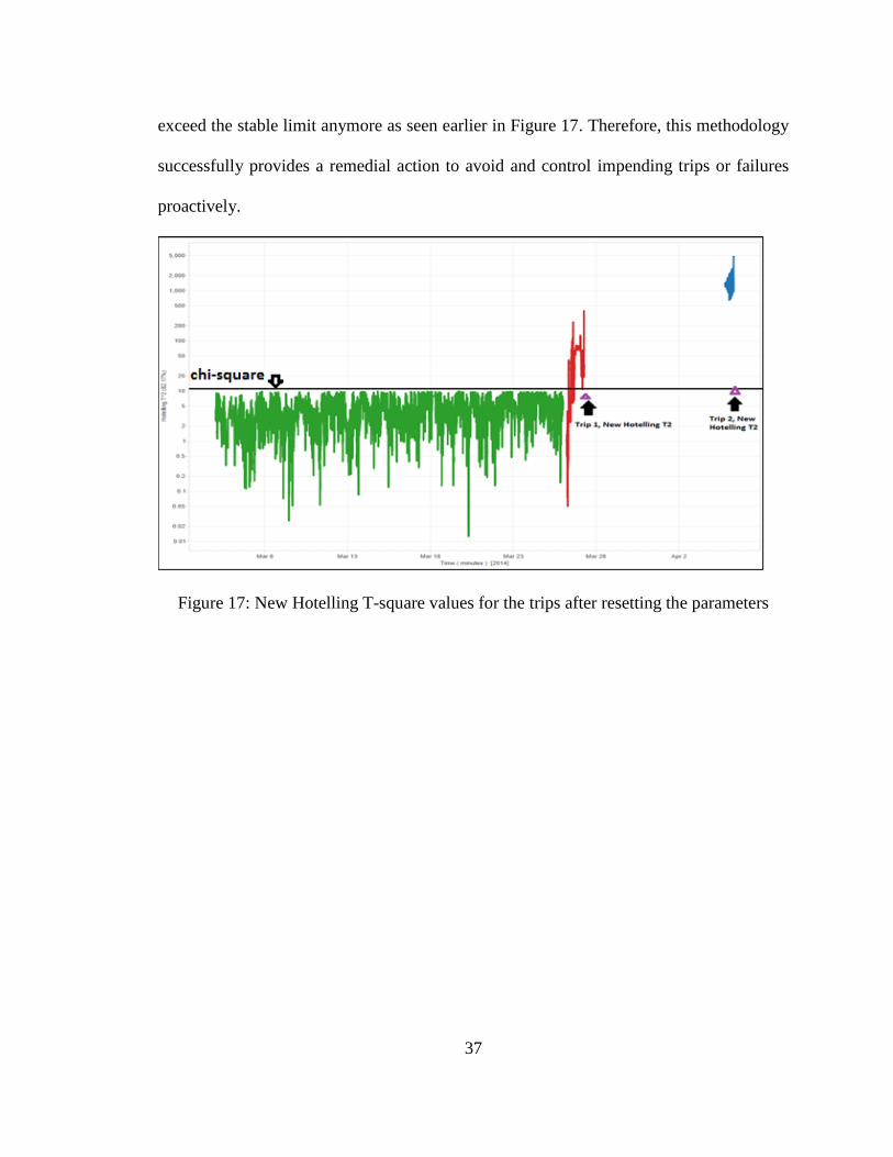
37
exceed the stable limit anymore as seen earlier in Figure 17. Therefore, this methodology
successfully provides a remedial action to avoid and control impending trips or failures
proactively.
Figure 17: New Hotelling T-square values for the trips after resetting the parameters

38
CHAPTER 6
CONCLUSION AND RECOMMENDATIONS
6.1 Conclusion
A methodology for data-driven detection and diagnosis of impending ESP
problems in real time has been proposed using Principal Component Analysis (PCA)
dimensionality reduction technique. It creates an opportunity to advance from a reactive
approach towards a more proactive approach based on predictive analysis, detection of an
impending problem, diagnosis of the cause of the impending problem, and prescription of
preventive action that will avoid or at least mitigate the impending problem.
In building the predictive model, historical data was used to determine and
evaluate key operational variables (decision variables) that affect ESP performance.
Based on historical data, a hybrid approach (combination of first principles and empirical
statistics) was used to develop Principal Component Analysis model to capture trends and
patterns in the behavior of ESPs. Trends or patterns during normal operation were
identified and correlated to either satisfactory operation or impending problems. Six
principal components obtained from the model output were sufficient to capture more
than 96% of observed variance with 95% confidence limit. It can identify patterns in data
based on scores and Hotelling T-square statistic and correlate them with normal operation
or impending event. The model was further enhanced to identify key parameters
contributing to impending failure. It eventually prescribes stable operating ranges for
each parameter, thereby prescribing remedial action to mitigate and/ or prevent failure.

39
With this tool, there would be ample time to take preventive action that could mitigate or
altogether avoid each problem.
6.2 Significance and Recommendations
This real-time analytical framework enables a shift towards proactive ESP
monitoring to identify impending problems long before they occur thereby safeguarding
ESP operation, reducing intervention costs and optimizing production. This approach
creates opportunities to increase pump uptime, extend the life expectancy of ESPs and
improve oilfield economics.
There are opportunities to extend the mathematical model to attribute different
categories of failure or abnormal behavior like high gas, corrosion, electrical problems to
different forms of patterns or clusters. This methodology can also be tested against other
mechanical systems or other forms of artificial lift technology.

40
REFERENCES
1) Bates R., Cosad C., Fielder L., Kosmala A., Hudson S., Romero G. and
Shanmugam V., “Taking the Pulse of Producing Wells-ESP Surveillance,”
Oilfield Review 16, no.2 (Summer 2004):16-25.
2) Breit, S., and Ferrier, N., "Electric Submersible Pumps in the Oil and Gas
Industry." Pumps & Systems. Wood Group ESP, Inc., Apr. 2008. Web. 26 Aug.
2014. Retrieved from http://www.pump-zone.com/topics/pumps/pumps/electric-
submersible-pumps-oil-and-gas-industry
3) Romero, O.J., Hupp, A. 2013 Subsea Electrical Submersible Pump Significance
in Petroleum Offshore Production, J. Energy Resources Technology 136(1): 1–8.
4) Spears & Associates, "Oilfield Market Report, 1999-2010," Tulsa, 2009.
5) Vandevier, J. (2010). “Run-Time Analysis Assesses Pump Performance.” Oil and
Gas Journal 108.37; pp. 76-79.
6) Holdaway, Keith R., (2014). Harness Oil and Gas Big Data With Analytics:
Optimize Exploration and Production With Data-Driven Models, New Jersey,
NY: John Wiley & Sons.
7) Carrillo, W. (2013). “Prognostics for Oil & Gas Artificial Lift applications.” GE
Oil & Gas, PHM Conference, New Orleans (2013). Retrieved from
https://www.phmsociety.org/sites/phmsociety.org/files/HMOG_01_GE.pdf
8) Camilleri, L. A. P., & Zhou, W. (2011, January 1). Obtaining Real-Time Flow
Rate, Water Cut, and Reservoir Diagnostics from ESP Gauge Data. Paper SPE
145542-MS presented at Offshore Europe Oil & Gas Conference and Exhibition,
6-8 September, Aberdeen, UK

41
9) Gabor Takacs, 2009, “Electrical Submersible Pumps Manual: Design, Operations,
and Maintenance”(pp.63, 99, 323-338), Gulf Professional Publishing, Elsevier,
Oxford, UK
10) Rider, J. and Dubue, R.: “Troubleshooting ESP Systems using Intelligent
Controls.” Paper presented at the ESP Workshop held in Houston, Texas, April
26–28, 2000.
11) Bravo, C., Rodriguez, J., Saputelli, L., & Rivas Echevarria, F. (2014, April 1).
Applying Analytics to Production Workflows: Transforming Integrated
Operations into Intelligent Operations. Paper SPE 167823-MS presented at the
SPE Intelligent Energy Conference & Exhibition, 1-3 April, Utrecht, The
Netherlands
12) Al-Jasmi, A., Nasr, H., Goel, H. K., Moricca, G., Carvajal, G. A., Dhar , J.,
Querales, M., Villamizar, M. A. , Cullick, A. S. , Rodriguez, J. A. , Velasquez, G.,
Yong, Z. , Bermudez, F. , Kain J,(2013). ESP “Smart Flow” Integrates Quality
and Control Data for Diagnostics and Optimization in Real Time. Paper SPE
163809 presented at the SPE Digital Energy Conference, The Woodlands, Texas,
USA, 05-07 March.
13) Bertocco, R., Padmanabhan,V. (2014, March 26). “Big Data analytics in Oil and
gas.” Bain & Company. Retrieved from
http://www.bain.com/Images/BAIN_BRIEF_Big_Data_analytics_in_oil_and_gas.

42
14) Derrick, T., Gavia, J., Jenkins, C., Oster, C., Sandlin, J., and Wright, K. 2013.
Analytics beyond R2: Year one. Paper SPE 163713 presented at the SPE Digital
Energy Conference and Exhibition, The Woodlands, TX, 5–7 March.
15) Stone, P. 2007. Introducing Predictive Analytics: Opportunities. Paper SPE
106865 presented at the SPE Digital Energy Conference and Exhibition, Houston,
Texas, 11–22 April.
16) Brule, M. R. 2013. Big Data in E&P: Real-time adaptive analytics and data flow
architecture. Paper SPE 163721 presented at the Digital Energy Conference and
Exhibition, The Woodlands, Texas, 5–7 March.
17) Bertolucci, J. (2013, December 31). “Big Data Analytics: Descriptive Vs.
Predictive Vs. Prescriptive.” Post, InformationWeek. Retrieved from
http://www.informationweek.com/big-data/big-data-analytics/big-data-analytics-
descriptive-vs-predictive-vs-prescriptive/d/d-id/1113279
18) Jackson, J.E. (1991). A User's Guide to Principal Components (Wiley).
19) Hubert M., Rousseeuw P. J., Branden K. V. (2005), ROBPCA: a new approach to
robust principal components analysis, Technometrics, 47, 64–79.
20) Westerhuis J., Gurden S., and Smilde A., Generalized contribution plots in
multivariate statistical process monitoring. Chemometrics and Intelligent
Laboratory Systems, vol. 51, pp. 95–114, 2000.
21) Paz-Kagan, T., Shachak, M., Zaady, E., Karnieli, A., 2014. A spectral soil quality
index (SSQI) for characterizing soil function in areas of changed land use.
Geoderma 230–231, 171–184

43
22) Nomikos P., Detection and diagnosis of abnormal batch operations based on
multi-way principal component analysis, ISA Trans. 35 (1996) 259–266.
23) Tracy N.D., Young J.C., Mason R.L., Multivariate control charts for individual
observations, J. Quality Technol. 24 (1992) 88–95.
24) Alexandersson, A. (2004), Graphing confidence ellipses: An update of ellip for
Stata 8, The Stata Journal, 4, 242-256.
25) Eriksson L, Johansson E, Kettaneh-Wold N, Wold S. Multi- and Megavariate
Data Analysis; Principles and Applications. Umetrics AB, Umeå, Sweden 2001,
ISBN 91-973730-1-X.

44
APPENDIX
A.1 Principal Component Analysis
Principal component analysis (PCA) is a statistical method to explain covariance
structure of data by means of a small number of components [19]. It converts a set of
possibly correlated variables into a set of linearly uncorrelated variables called Principal
components, enabling better understanding of the different sources of variation [18].
The classical PCA model is represented as
𝑋 = 𝑇𝑃𝑇 + 𝐸, (A.1-1)
where;
X is the input matrix (t by p),
T is the scores matrix (t by R); the scores matrix represents the relationship between
observations [25],
P is the loading matrix (p by R); it signifies the contribution and significance of the
parameters [25],
E is the residual matrix (t by p); it represents the variance not captured by the PCA
model,
where;
t = number of time steps,
p= number of parameters, and
R=number of principal components.
The first component corresponds to the direction in which variance in
observations projected on it is the largest [19]. The second component is orthogonal to
45
the first component and maximizes the variance of the data points projected on it.
Repeating this process of projecting observations onto orthogonal components yields all
principal components, corresponding to eigenvectors of the empirical covariance matrix
[19].
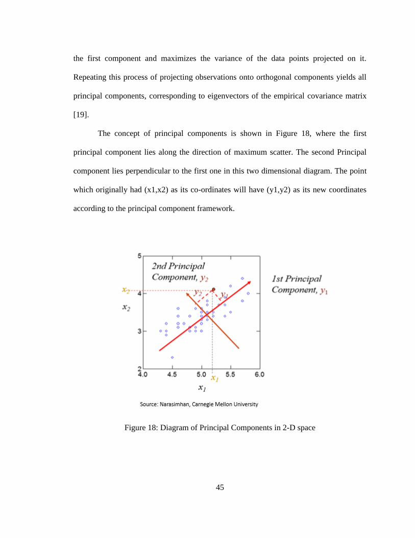
The concept of principal components is shown in Figure 18, where the first
principal component lies along the direction of maximum scatter. The second Principal
component lies perpendicular to the first one in this two dimensional diagram. The point
which originally had (x1,x2) as its co-ordinates will have (y1,y2) as its new coordinates
according to the principal component framework.
Figure 18: Diagram of Principal Components in 2-D space

46
Below are the steps which were performed while applying the PCA technique:
1. Standardize the data using the formula
𝑥𝑠𝑡𝑑 =𝑥−𝑚𝑒𝑎𝑛(𝑥)
𝑠𝑡𝑑 𝑑𝑒𝑣(𝑥). (A.1-2)
2. Calculate the covariance matrix to find the degree to which variables are linearly
correlated where
n
i
ii
n
xxxxxx
1
221121
1
))((),cov( . (A.1-3)
3. Calculate the eigenvalues which represent variations of the coordinates on each
Principal axis. The cross-product xx is first determined and eigenvalues are found
by finding the solution of the equation
0 IS . (A.1-4)
4. Calculate the eigenvectors. Each eigenvector consists of p values which
represents the contribution of each variable to the Principal Component axis
Eigenvectors are found by solving the equation
Ax= x, (A.1-5)
where x is the eigenvector and A is the transformed x data. The eigenvector
matrix is a pXR matrix and is represented by U.
5. The scores matrix represents the coordinates of each time step n on the Rth
principal component. The value of score for each principal component R at every
time step n is calculated using
npRiRnRRn xuxuxus 222211 . (A.1-6)
47
6. As a next step, the correlation between variables and PC’s are calculated and form
the loading matrix.
7. The % variance obtained by each eigenvector is calculated as the ratio of the
eigenvalue over the sum of all eigenvalues.
A.2 Robust Principal Component Analysis
The original input data in PCA is represented as t by p matrix X = Xt,p, where t =
number of time steps, and p = original number of decision variables. The Robust PCA
methodology has three steps as described by Hubert et al. (2005) [19].
Firstly, the data is preprocessed to ensure that transformed data lies in a subspace
whose dimension is less than p – 1.
Secondly, a preliminary covariance matrix 𝑜 is constructed and used for
selecting the number of components R that will be retained in the sequel, yielding
a R-dimensional subspace that fits the data well.
Finally, data points are projected on this subspace where their location and scatter
matrix are estimated, from which its R nonzero eigenvalues l1,l2 . . . , lR are
computed. The corresponding eigenvectors are the R robust principal
components.
In the original space of dimension p, these R components span an R-dimensional
subspace. The (column) eigenvectors if written next to one another yield the p by R
matrix Pp,R with orthogonal columns. The location estimate is represented by the p-
variate column vector µ̂, called the robust center. The scores are the t by R matrix
𝑇𝑡,𝑅 = (𝑋𝑡,𝑃 − 1𝑡µ̂′)𝑃𝑝,𝑅, (A.2-1)

48
where 1t is the column vector with all t components equal to 1. Moreover, the R robust
principal components generate a p by p robust scatter matrix of rank R given by
= 𝑃𝑝,𝑅𝐿𝑅,𝑅𝑃𝑝,𝑅′ , (A.2-2)
where LR,R is the diagonal matrix with the eigenvalues l1,l2 . . . , lR.

49