contentsphysics.ucsd.edu/.../courses/fall2013/physics210b/lectures/ch05.pdf · contents 5 the...

Contents

5 The Boltzmann Equation 1

5.1 References . . . . . . . . . . . . . . . . . . . . . . . . . . . . . . . . . . . . . . . . . . . . . . . . . . . . 1

5.2 Equilibrium, Nonequilibrium and Local Equilibrium . . . . . . . . . . . . . . . . . . . . . . . . . . . 2

5.3 Boltzmann Transport Theory . . . . . . . . . . . . . . . . . . . . . . . . . . . . . . . . . . . . . . . . . 3

5.3.1 Derivation of the Boltzmann equation . . . . . . . . . . . . . . . . . . . . . . . . . . . . . . . 3

5.3.2 Collisionless Boltzmann equation . . . . . . . . . . . . . . . . . . . . . . . . . . . . . . . . . . 5

5.3.3 Collisional invariants . . . . . . . . . . . . . . . . . . . . . . . . . . . . . . . . . . . . . . . . . 6

5.3.4 Scattering processes . . . . . . . . . . . . . . . . . . . . . . . . . . . . . . . . . . . . . . . . . . 7

5.3.5 Detailed balance . . . . . . . . . . . . . . . . . . . . . . . . . . . . . . . . . . . . . . . . . . . . 8

5.3.6 Kinematics and cross section . . . . . . . . . . . . . . . . . . . . . . . . . . . . . . . . . . . . . 10

5.3.7 H-theorem . . . . . . . . . . . . . . . . . . . . . . . . . . . . . . . . . . . . . . . . . . . . . . . 10

5.4 Weakly Inhomogeneous Gas . . . . . . . . . . . . . . . . . . . . . . . . . . . . . . . . . . . . . . . . . 12

5.5 Relaxation Time Approximation . . . . . . . . . . . . . . . . . . . . . . . . . . . . . . . . . . . . . . . 14

5.5.1 Approximation of collision integral . . . . . . . . . . . . . . . . . . . . . . . . . . . . . . . . . 14

5.5.2 Computation of the scattering time . . . . . . . . . . . . . . . . . . . . . . . . . . . . . . . . . 14

5.5.3 Thermal conductivity . . . . . . . . . . . . . . . . . . . . . . . . . . . . . . . . . . . . . . . . . 15

5.5.4 Viscosity . . . . . . . . . . . . . . . . . . . . . . . . . . . . . . . . . . . . . . . . . . . . . . . . 16

5.5.5 Oscillating external force . . . . . . . . . . . . . . . . . . . . . . . . . . . . . . . . . . . . . . . 19

5.5.6 Quick and Dirty Treatment of Transport . . . . . . . . . . . . . . . . . . . . . . . . . . . . . . 20

5.5.7 Thermal diffusivity, kinematic viscosity, and Prandtl number . . . . . . . . . . . . . . . . . . 20

5.6 Diffusion and the Lorentz model . . . . . . . . . . . . . . . . . . . . . . . . . . . . . . . . . . . . . . . 21

5.6.1 Failure of the relaxation time approximation . . . . . . . . . . . . . . . . . . . . . . . . . . . . 21

5.6.2 Modified Boltzmann equation and its solution . . . . . . . . . . . . . . . . . . . . . . . . . . 22

i

ii CONTENTS

5.7 Linearized Boltzmann Equation . . . . . . . . . . . . . . . . . . . . . . . . . . . . . . . . . . . . . . . 24

5.7.1 Linearizing the collision integral . . . . . . . . . . . . . . . . . . . . . . . . . . . . . . . . . . . 24

5.7.2 Linear algebraic properties of L . . . . . . . . . . . . . . . . . . . . . . . . . . . . . . . . . . . 24

5.7.3 Steady state solution to the linearized Boltzmann equation . . . . . . . . . . . . . . . . . . . 26

5.7.4 Variational approach . . . . . . . . . . . . . . . . . . . . . . . . . . . . . . . . . . . . . . . . . 26

5.8 The Equations of Hydrodynamics . . . . . . . . . . . . . . . . . . . . . . . . . . . . . . . . . . . . . . 30

5.9 Nonequilibrium Quantum Transport . . . . . . . . . . . . . . . . . . . . . . . . . . . . . . . . . . . . 30

5.9.1 Boltzmann equation for quantum systems . . . . . . . . . . . . . . . . . . . . . . . . . . . . . 30

5.9.2 The Heat Equation . . . . . . . . . . . . . . . . . . . . . . . . . . . . . . . . . . . . . . . . . . . 34

5.9.3 Calculation of Transport Coefficients . . . . . . . . . . . . . . . . . . . . . . . . . . . . . . . . 35

5.9.4 Onsager Relations . . . . . . . . . . . . . . . . . . . . . . . . . . . . . . . . . . . . . . . . . . . 36

5.10 Appendix : Boltzmann Equation and Collisional Invariants . . . . . . . . . . . . . . . . . . . . . . . 37

Chapter 5

The Boltzmann Equation

5.1 References

– H. Smith and H. H. Jensen, Transport Phenomena (Oxford, 1989)An outstanding, thorough, and pellucid presentation of the theory of Boltzmann transport in classical andquantum systems.

– P. L. Krapivsky, S. Redner, and E. Ben-Naim, A Kinetic View of Statistical Physics (Cambridge, 2010)Superb, modern discussion of a broad variety of issues and models in nonequilibrium statistical physics.

– E. M. Lifshitz and L. P. Pitaevskii, Physical Kinetics (Pergamon, 1981)Volume 10 in the famous Landau and Lifshitz Course of Theoretical Physics. Surprisingly readable, andwith many applications (some advanced).

– M. Kardar, Statistical Physics of Particles (Cambridge, 2007)A superb modern text, with many insightful presentations of key concepts. Includes a very instructivederivation of the Boltzmann equation starting from the BBGKY hierarchy.

– J. A. McLennan, Introduction to Non-equilibrium Statistical Mechanics (Prentice-Hall, 1989)Though narrow in scope, this book is a good resource on the Boltzmann equation.

– F. Reif, Fundamentals of Statistical and Thermal Physics (McGraw-Hill, 1987)This has been perhaps the most popular undergraduate text since it first appeared in 1967, and with goodreason. The later chapters discuss transport phenomena at an undergraduate level.

– N. G. Van Kampen, Stochastic Processes in Physics and Chemistry (3rd edition, North-Holland, 2007)This is a very readable and useful text. A relaxed but meaty presentation.

1

2 CHAPTER 5. THE BOLTZMANN EQUATION

5.2 Equilibrium, Nonequilibrium and Local Equilibrium

Classical equilibrium statistical mechanics is described by the full N -body distribution,

f0(x1, . . . ,xN ; p1, . . . ,pN ) =

Z−1N · 1

N ! e−βHN (p,x) OCE

Ξ−1 · 1N ! e

βµNe−βHN (p,x) GCE .

(5.1)

We assume a Hamiltonian of the form

HN =

N∑

i=1

p2i

2m+

N∑

i=1

v(xi) +

N∑

i<j

u(xi − xj), (5.2)

typically with v = 0, i.e. only two-body interactions. The quantity

f0(x1, . . . ,xN ; p1, . . . ,pN )ddx1 d

dp1

hd· · · d

dxN ddpNhd

(5.3)

is the probability, under equilibrium conditions, of finding N particles in the system, with particle #1 lying within

d3x1 of x1 and having momentum within ddp1 of p1, etc. The temperature T and chemical potential µ are constants,independent of position. Note that f(xi, pi) is dimensionless.

Nonequilibrium statistical mechanics seeks to describe thermodynamic systems which are out of equilibrium,meaning that the distribution function is not given by the Boltzmann distribution above. For a general nonequilib-rium setting, it is hopeless to make progress – we’d have to integrate the equations of motion for all the constituentparticles. However, typically we are concerned with situations where external forces or constraints are imposedover some macroscopic scale. Examples would include the imposition of a voltage drop across a metal, or a tem-perature differential across any thermodynamic sample. In such cases, scattering at microscopic length and timescales described by the mean free path ℓ and the collision time τ work to establish local equilibrium throughout thesystem. A local equilibrium is a state described by a space and time varying temperature T (r, t) and chemicalpotential µ(r, t). As we will see, the Boltzmann distribution with T = T (r, t) and µ = µ(r, t) will not be a solutionto the evolution equation governing the distribution function. Rather, the distribution for systems slightly out ofequilibrium will be of the form f = f0 + δf , where f0 describes a state of local equilibrium.

We will mainly be interested in the one-body distribution

f(r,p; t) =

N∑

i=1

⟨δ(xi(t) − r) δ(pi(t) − p

) ⟩

= N

∫ N∏

i=2

ddxi ddpi f(r,x2, . . . ,xN ; p,p2, . . . ,pN ; t) .

(5.4)

In this chapter, we will drop the 1/~ normalization for phase space integration. Thus, f(r,p, t) has dimensions ofh−d, and f(r,p, t) d3r d3p is the average number of particles found within d3r of r and d3p of p at time t.

In the GCE, we sum the RHS above over N . Assuming v = 0 so that there is no one-body potential to breaktranslational symmetry, the equilibrium distribution is time-independent and space-independent:

f0(r,p) = n (2πmkBT )−3/2 e−p2/2mkBT , (5.5)

where n = N/V or n = n(T, µ) is the particle density in the OCE or GCE. From the one-body distribution we can

5.3. BOLTZMANN TRANSPORT THEORY 3

compute things like the particle current, j, and the energy current, jε:

j(r, t) =

∫ddp f(r,p; t)

p

m(5.6)

jε(r, t) =

∫ddp f(r,p; t) ε(p)

p

m, (5.7)

where ε(p) = p2/2m. Clearly these currents both vanish in equilibrium, when f = f0, since f0(r,p) dependsonly on p2 and not on the direction of p. In a steady state nonequilibrium situation, the above quantities aretime-independent.

Thermodynamics says thatdq = T ds = dε− µdn , (5.8)

where s, ε, and n are entropy density, energy density, and particle density, respectively, and dq is the differentialheat density. This relation may be case as one among the corresponding current densities:

jq = T js = jε − µ j . (5.9)

Thus, in a system with no particle flow, j = 0 and the heat current jq is the same as the energy current jε.

When the individual particles are not point particles, they possess angular momentum as well as linear momen-tum. Following Lifshitz and Pitaevskii, we abbreviate Γ = (p,L) for these two variables for the case of diatomicmolecules, and Γ = (p,L, n · L) in the case of spherical top molecules, where n is the symmetry axis of the top.We then have, in d = 3 dimensions,

dΓ =

d3p point particles

d3p L dL dΩL diatomic molecules

d3p L2 dL dΩL d cosϑ symmetric tops ,

(5.10)

where ϑ = cos−1(n · L). We will call the set Γ the ‘kinematic variables’. The instantaneous number density at r isthen

n(r, t) =

∫dΓ f(r, Γ ; t) . (5.11)

One might ask why we do not also keep track of the angular orientation of the individual molecules. There aretwo reasons. First, the rotations of the molecules are generally extremely rapid, so we are justified in averagingover these motions. Second, the orientation of, say, a rotor does not enter into its energy. While the same can besaid of the spatial position in the absence of external fields, (i) in the presence of external fields one must keeptrack of the position coordinate r since there is physical transport of particles from one region of space to another,and (iii) the collision process, which as we shall see enters the dynamics of the distribution function, takes placein real space.

5.3 Boltzmann Transport Theory

5.3.1 Derivation of the Boltzmann equation

For simplicity of presentation, we assume point particles. Recall that

f(r,p, t) d3r d3p ≡

# of particles with positions within d3r of

r and momenta within d3p of p at time t.(5.12)


We now ask how the distribution functions f(r,p, t) evolves in time. It is clear that in the absence of collisions,the distribution function must satisfy the continuity equation,

∂f

∂t+ ∇·(uf) = 0 . (5.13)

This is just the condition of number conservation for particles. Take care to note that ∇ and u are six-dimensionalphase space vectors:

u = ( x , y , z , px , py , pz ) (5.14)

∇ =

(∂

∂x,∂

∂y,∂

∂z,∂

∂px,∂

∂py,∂

∂pz

). (5.15)

The continuity equation describes a distribution in which each constituent particle evolves according to a pre-scribed dynamics, which for a mechanical system is specified by

dr

dt=∂H

∂p= v(p) ,

dp

dt= −∂H

∂r= Fext , (5.16)

where F is an external applied force. Here,

H(p, r) = ε(p) + Uext(r) . (5.17)

For example, if the particles are under the influence of gravity, then Uext(r) = mg · r and F = −∇Uext = −mg.

Note that as a consequence of the dynamics, we have ∇ ·u = 0, i.e. phase space flow is incompressible, providedthat ε(p) is a function of p alone, and not of r. Thus, in the absence of collisions, we have

∂f

∂t+ u ·∇f = 0 . (5.18)

The differential operator Dt ≡ ∂t + u ·∇ is sometimes called the ‘convective derivative’, because Dtf is the timederivative of f in a comoving frame of reference.

Next we must consider the effect of collisions, which are not accounted for by the semiclassical dynamics. In acollision process, a particle with momentum p and one with momentum p can instantaneously convert into a pairwith momenta p′ and p′, provided total momentum is conserved: p + p = p′ + p′. This means that Dtf 6= 0.Rather, we should write

∂f

∂t+ r · ∂f

∂r+ p · ∂f

∂p=

(∂f

∂t

)

coll

(5.19)

where the right side is known as the collision integral. The collision integral is in general a function of r, p, and tand a functional of the distribution f .

After a trivial rearrangement of terms, we can write the Boltzmann equation as

∂f

∂t=

(∂f

∂t

)

str

+

(∂f

∂t

)

coll

, (5.20)

where (∂f

∂t

)

str

≡ −r · ∂f∂r

− p · ∂f∂p

(5.21)

is known as the streaming term. Thus, there are two contributions to ∂f/∂t : streaming and collisions.


5.3.2 Collisionless Boltzmann equation

In the absence of collisions, the Boltzmann equation is given by

∂f

∂t+∂ε

∂p· ∂f∂r

− ∇Uext ·∂f

∂p= 0 . (5.22)

In order to gain some intuition about how the streaming term affects the evolution of the distribution f(r,p, t),consider a case where Fext = 0. We then have

∂f

∂t+

p

m· ∂f∂r

= 0 . (5.23)

Clearly, then, any function of the form

f(r,p, t) = ϕ(r − v(p) t , p

)(5.24)

will be a solution to the collisionless Boltzmann equation, where v(p) = ∂ε∂p . One possible solution would be the

Boltzmann distribution,

f(r,p, t) = eµ/kBT e−p2/2mkBT , (5.25)

which is time-independent1. Here we have assumed a ballistic dispersion, ε(p) = p2/2m.

For a slightly less trivial example, let the initial distribution be ϕ(r,p) = Ae−r2/2σ2

e−p2/2κ2

, so that

f(r,p, t) = Ae−(r− pt

m

)2/2σ2

e−p2/2κ2

. (5.26)

Consider the one-dimensional version, and rescale position, momentum, and time so that

f(x, p, t) = Ae−12 (x−p t)2 e−

12 p2

. (5.27)

Consider the level sets of f , where f(x, p, t) = Ae−12α2

. The equation for these sets is

x = p t±√α2 − p2 . (5.28)

For fixed t, these level sets describe the loci in phase space of equal probability densities, with the probabilitydensity decreasing exponentially in the parameter α2. For t = 0, the initial distribution describes a Gaussiancloud of particles with a Gaussian momentum distribution. As t increases, the distribution widens in x but notin p – each particle moves with a constant momentum, so the set of momentum values never changes. However,the level sets in the (x , p) plane become elliptical, with a semimajor axis oriented at an angle θ = ctn−1(t) withrespect to the x axis. For t > 0, he particles at the outer edges of the cloud are more likely to be moving away fromthe center. See the sketches in fig. 5.1

Suppose we add in a constant external force Fext. Then it is easy to show (and left as an exercise to the reader toprove) that any function of the form

f(r,p, t) = Aϕ

(r − p t

m+

Fextt2

2m, p − Fextt

m

)(5.29)

satisfies the collisionless Boltzmann equation (ballistic dispersion assumed).

1Indeed, any arbitrary function of p alone would be a solution. Ultimately, we require some energy exchanging processes, such as collisions,in order for any initial nonequilibrium distribution to converge to the Boltzmann distribution.


Figure 5.1: Level sets for a sample f(x, p, t) = Ae−12 (x−pt)2e−

12 p2

, for values f = Ae−12α2

with α in equally spacedintervals from α = 0.2 (red) to α = 1.2 (blue). The time variable t is taken to be t = 0.0 (upper left), 0.2 (upperright), 0.8 (lower right), and 1.3 (lower left).

5.3.3 Collisional invariants

Consider a function A(r,p) of position and momentum. Its average value at time t is

A(t) =

∫d3r d3p A(r,p) f(r,p, t) . (5.30)

Taking the time derivative,

dA

dt=

∫d3r d3p A(r,p)

∂f

∂t

=

∫d3r d3p A(r,p)

− ∂

∂r· (rf) − ∂

∂p· (pf) +

(∂f

∂t

)

coll

=

∫d3r d3p

(∂A

∂r· drdt

+∂A

∂p· dpdt

)f +A(r,p)

(∂f

∂t

)

coll

.

(5.31)

Hence, if A is preserved by the dynamics between collisions, then2

dA

dt=∂A

∂r· drdt

+∂A

∂p· dpdt

= 0 . (5.32)

2Recall from classical mechanics the definition of the Poisson bracket, A, B = ∂A∂r · ∂B

∂p − ∂B∂r · ∂A

∂p . Then from Hamilton’s equations r = ∂H∂p

and p = − ∂H∂r , where H(p,r, t) is the Hamiltonian, we have dA

dt= A, H. Invariants have zero Poisson bracket with the Hamiltonian.


We therefore have that the rate of change of A is determined wholly by the collision integral

dA

dt=

∫d3r d3p A(r,p)

(∂f

∂t

)

coll

. (5.33)

Quantities which are then conserved in the collisions satisfy A = 0. Such quantities are called collisional invariants.Examples of collisional invariants include the particle number (A = 1), the components of the total momentum(A = pµ) (in the absence of broken translational invariance, due e.g. to the presence of walls), and the total energy(A = ε(p)).

5.3.4 Scattering processes

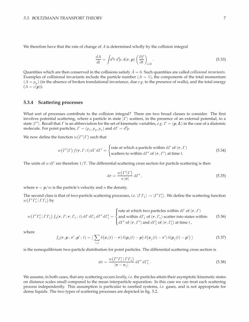
What sort of processes contribute to the collision integral? There are two broad classes to consider. The firstinvolves potential scattering, where a particle in state |Γ 〉 scatters, in the presence of an external potential, to astate |Γ ′〉. Recall that Γ is an abbreviation for the set of kinematic variables, e.g. Γ = (p,L) in the case of a diatomicmolecule. For point particles, Γ = (px, py, pz) and dΓ = d3p.

We now define the function w(Γ ′|Γ

)such that

w(Γ ′|Γ

)f(r, Γ ; t) dΓ dΓ ′ =

rate at which a particle within dΓ of (r, Γ )

scatters to within dΓ ′ of (r, Γ ′) at time t.(5.34)

The units of w dΓ are therefore 1/T . The differential scattering cross section for particle scattering is then

dσ =w(Γ ′|Γ

)

n |v| dΓ ′ , (5.35)

where v = p/m is the particle’s velocity and n the density.

The second class is that of two-particle scattering processes, i.e. |ΓΓ1〉 → |Γ ′Γ ′1〉. We define the scattering function

w(Γ ′Γ ′

1 |ΓΓ1

)by

w(Γ ′Γ ′

1 |ΓΓ1

)f2(r, Γ ; r, Γ1 ; t) dΓ dΓ1 dΓ

′ dΓ ′1 =

rate at which two particles within dΓ of (r, Γ )

and within dΓ1 of (r, Γ1) scatter into states within

dΓ ′ of (r, Γ ′) and dΓ ′1 of (r, Γ ′

1) at time t ,

(5.36)

where

f2(r,p ; r′,p′ ; t) =⟨∑

i,j

δ(xi(t) − r) δ(pi(t) − p

)δ(xj(t) − r′) δ(pj(t) − p′) ⟩ (5.37)

is the nonequilibrium two-particle distribution for point particles. The differential scattering cross section is

dσ =w(Γ ′Γ ′

1 |ΓΓ1

)

|v − v1|dΓ ′ dΓ ′

1 . (5.38)

We assume, in both cases, that any scattering occurs locally, i.e. the particles attain their asymptotic kinematic stateson distance scales small compared to the mean interparticle separation. In this case we can treat each scatteringprocess independently. This assumption is particular to rarefied systems, i.e. gases, and is not appropriate fordense liquids. The two types of scattering processes are depicted in fig. 5.2.


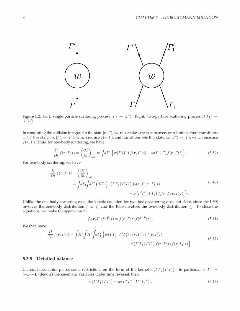
Figure 5.2: Left: single particle scattering process |Γ 〉 → |Γ ′〉. Right: two-particle scattering process |ΓΓ1〉 →|Γ ′Γ ′

1〉.

In computing the collision integral for the state |r, Γ 〉, we must take care to sum over contributions from transitionsout of this state, i.e. |Γ 〉 → |Γ ′〉, which reduce f(r, Γ ), and transitions into this state, i.e. |Γ ′〉 → |Γ 〉, which increasef(r, Γ ). Thus, for one-body scattering, we have

D

Dtf(r, Γ ; t) =

(∂f

∂t

)

coll

=

∫dΓ ′

w(Γ |Γ ′) f(r, Γ ′; t) − w(Γ ′ |Γ ) f(r, Γ ; t)

. (5.39)

For two-body scattering, we have

D

Dtf(r, Γ ; t) =

(∂f

∂t

)

coll

=

∫dΓ1

∫dΓ ′∫dΓ ′

1

w(ΓΓ1 |Γ ′Γ ′

1

)f2(r, Γ

′; r, Γ ′1; t)

− w(Γ ′Γ ′

1 |ΓΓ1

)f2(r, Γ ; r, Γ1; t)

.

(5.40)

Unlike the one-body scattering case, the kinetic equation for two-body scattering does not close, since the LHSinvolves the one-body distribution f ≡ f1 and the RHS involves the two-body distribution f2. To close theequations, we make the approximation

f2(r, Γ′; r, Γ ; t) ≈ f(r, Γ ; t) f(r, Γ ; t) . (5.41)

We then have

D

Dtf(r, Γ ; t) =

∫dΓ1


1

w(ΓΓ1 |Γ ′Γ ′

1

)f(r, Γ ′; t) f(r, Γ ′

1; t)

− w(Γ ′Γ ′

1 |ΓΓ1

)f(r, Γ ; t) f(r, Γ1; t)

.

(5.42)

5.3.5 Detailed balance

Classical mechanics places some restrictions on the form of the kernel w(ΓΓ1 |Γ ′Γ ′

1

). In particular, if Γ T =

(−p,−L) denotes the kinematic variables under time reversal, then

w(Γ ′Γ ′

1 |ΓΓ1

)= w

(Γ TΓ T

1 |Γ ′TΓ ′1

T). (5.43)


This is because the time reverse of the process |ΓΓ1〉 → |Γ ′Γ ′1〉 is |Γ ′TΓ ′

1T〉 → |Γ TΓ T

1 〉.

In equilibrium, we must have

w(Γ ′Γ ′

1 |ΓΓ1

)f0(Γ ) f0(Γ1) d

4Γ = w(Γ TΓ T

1 |Γ ′TΓ ′1

T)f0(Γ ′T ) f0(Γ ′

1T ) d4Γ T (5.44)

whered4Γ ≡ dΓ dΓ1 dΓ

′dΓ ′1 , d4Γ T ≡ dΓ T dΓ T

1 dΓ′TdΓ ′

1T . (5.45)

Since dΓ = dΓ T etc., we may cancel the differentials above, and after invoking eqn. 5.43 and suppressing thecommon r label, we find

f0(Γ ) f0(Γ1) = f0(Γ ′T ) f0(Γ ′1

T ) . (5.46)

This is the condition of detailed balance. For the Boltzmann distribution, we have

f0(Γ ) = Ae−ε/kBT , (5.47)

where A is a constant and where ε = ε(Γ ) is the kinetic energy, e.g. ε(Γ ) = p2/2m in the case of point particles.Note that ε(Γ T ) = ε(Γ ). Detailed balance is satisfied because the kinematics of the collision requires energyconservation:

ε+ ε1 = ε′ + ε′1 . (5.48)

Since momentum is also kinematically conserved, i.e.

p + p1 = p′ + p′1 , (5.49)

any distribution of the form

f0(Γ ) = Ae−(ε−p·V )/kBT (5.50)

also satisfies detailed balance, for any velocity parameter V . This distribution is appropriate for gases which areflowing with average particle V .

In addition to time-reversal, parity is also a symmetry of the microscopic mechanical laws. Under the parityoperation P , we have r → −r and p → −p. Note that a pseudovector such as L = r × p is unchanged underP . Thus, Γ P = (−p,L). Under the combined operation of C = PT , we have ΓC = (p,−L). If the microscopicHamiltonian is invariant under C, then we must have

w(Γ ′Γ ′

1 |ΓΓ1

)= w

(ΓCΓC

1 |Γ ′CΓ ′1

C). (5.51)

For point particles, invariance under T and P then means

w(p′,p′1 |p,p1) = w(p,p1 |p′,p′

1) , (5.52)

and therefore the collision integral takes the simplified form,

Df(p)

Dt=

(∂f

∂t

)

coll

=

∫d3p1

∫d3p′∫d3p′1 w(p′,p′

1 |p,p1)f(p′) f(p′

1) − f(p) f(p1),

(5.53)

where we have suppressed both r and t variables.

The most general statement of detailed balance is

f0(Γ ′) f0(Γ ′1)

f0(Γ ) f0(Γ1)=w(Γ ′Γ ′

1 |ΓΓ1

)

w(ΓΓ1 |Γ ′Γ ′

1

) . (5.54)

Under this condition, the collision term vanishes for f = f0, which is the equilibrium distribution.


5.3.6 Kinematics and cross section

We can rewrite eqn. 5.53 in the form

Df(p)

Dt=

∫d3p1

∫dΩ |v − v1|

∂σ

∂Ω

f(p′) f(p′

1) − f(p) f(p1), (5.55)

where ∂σ∂Ω is the differential scattering cross section. If we recast the scattering problem in terms of center-of-mass

and relative coordinates, we conclude that the total momentum is conserved by the collision, and furthermore thatthe energy in the CM frame is conserved, which means that the magnitude of the relative momentum is conserved.

Thus, we may write p′ − p′1 = |p − p1| Ω, where Ω is a unit vector. Then p′ and p′

1 are determined to be

p′ = 12

(p + p1 + |p − p1| Ω

)

p′1 = 1

2

(p + p1 − |p − p1| Ω

).

(5.56)

5.3.7 H-theorem

Let’s consider the Boltzmann equation with two particle collisions. We define the local (i.e. r-dependent) quantity

ρϕ(r, t) ≡∫dΓ ϕ(Γ, f) f(Γ, r, t) . (5.57)

At this point, ϕ(Γ, f) is arbitrary. Note that the ϕ(Γ, f) factor has r and t dependence through its dependence onf , which itself is a function of r, Γ , and t. We now compute

∂ρϕ

∂t=

∫dΓ

∂(ϕf)

∂t=

∫dΓ

∂(ϕf)

∂f

∂f

∂t

= −∫dΓ u · ∇(ϕf) −

∫dΓ

∂(ϕf)

∂f

(∂f

∂t

)

coll

= −∮dΣ n · (uϕf) −

∫dΓ

∂(ϕf)

∂f

(∂f

∂t

)

coll

.

(5.58)

The first term on the last line follows from the divergence theorem, and vanishes if we assume f = 0 for infinitevalues of the kinematic variables, which is the only physical possibility. Thus, the rate of change of ρϕ is entirelydue to the collision term. Thus,

∂ρϕ

∂t=

∫dΓ

∫dΓ1


1

w(Γ ′Γ ′

1 |ΓΓ1

)ff1 χ− w

(ΓΓ1 |Γ ′Γ ′

1

)f ′f ′

1 χ

=

∫dΓ

∫dΓ1


1 w(Γ ′Γ ′

1 |ΓΓ1

)ff1 (χ− χ′) ,

(5.59)

where f ≡ f(Γ ), f ′ ≡ f(Γ ′), f1 ≡ f(Γ1), f′1 ≡ f(Γ ′

1), χ = χ(Γ ), with

χ =∂(ϕf)

∂f= ϕ+ f

∂ϕ

∂f. (5.60)

We now invoke the symmetryw(Γ ′Γ ′

1 |ΓΓ1

)= w

(Γ ′

1 Γ′ |Γ1 Γ

), (5.61)

which allows us to write

∂ρϕ

∂t= 1

2

∫dΓ

∫dΓ1


1 w(Γ ′Γ ′

1 |ΓΓ1

)ff1 (χ+ χ1 − χ′ − χ′

1) . (5.62)


This shows that ρϕ is preserved by the collision term if χ(Γ ) is a collisional invariant.

Now let us consider ϕ(f) = ln f . We define h ≡ ρ∣∣ϕ=ln f

. We then have

∂h

∂t= − 1

2

∫dΓ

∫dΓ1


1 w f′f ′

1 · x lnx , (5.63)

where w ≡ w(Γ ′Γ ′

1 |ΓΓ1

)and x ≡ ff1/f

′f ′1. We next invoke the result


1 w(Γ ′Γ ′

1 |ΓΓ1

)=


1 w(ΓΓ1 |Γ ′Γ ′

1

)(5.64)

which is a statement of unitarity of the scattering matrix3. Multiplying both sides by f(Γ ) f(Γ1), then integratingover Γ and Γ1, and finally changing variables (Γ, Γ1) ↔ (Γ ′, Γ ′

1), we find

0 =

∫dΓ

∫dΓ1


1 w(ff1 − f ′f ′

1

)=

∫dΓ

∫dΓ1


1 w f′f ′

1 (x − 1) . (5.65)

Multiplying this result by 12 and adding it to the previous equation for h, we arrive at our final result,

∂h

∂t= − 1

2

∫dΓ

∫dΓ1


1 w f′f ′

1 (x ln x− x+ 1) . (5.66)

Note that w, f ′, and f ′1 are all nonnegative. It is then easy to prove that the function g(x) = x ln x − x + 1 is

nonnegative for all positive x values4, which therefore entails the important result

∂h(r, t)

∂t≤ 0 . (5.67)

Boltzmann’s H function is the space integral of the h density: H =∫d3r h.

Thus, everywhere in space, the function h(r, t) is monotonically decreasing or constant, due to collisions. In

equilibrium, h = 0 everywhere, which requires x = 1, i.e.

f0(Γ ) f0(Γ1) = f0(Γ ′) f0(Γ ′1) , (5.68)

or, taking the logarithm,

ln f0(Γ ) + ln f0(Γ1) = ln f0(Γ ′) + ln f0(Γ ′1) . (5.69)

But this means that ln f0 is itself a collisional invariant, and if 1, p, and ε are the only collisional invariants, thenln f0 must be expressible in terms of them. Thus,

ln f0 =µ

kBT

+V ·pk

BT

− ε

kBT, (5.70)

where µ, V , and T are constants which parameterize the equilibrium distribution f0(p), corresponding to thechemical potential, flow velocity, and temperature, respectively.

3See Lifshitz and Pitaevskii, Physical Kinetics, §2.4The function g(x) = x ln x − x + 1 satisfies g′(x) = ln x, hence g′(x) < 0 on the interval x ∈ [0, 1) and g′(x) > 0 on x ∈ (1,∞]. Thus,

g(x) monotonically decreases from g(0) = 1 to g(1) = 0, and then monotonically increases to g(∞) = ∞, never becoming negative.


5.4 Weakly Inhomogeneous Gas

Consider a gas which is only weakly out of equilibrium. We follow the treatment in Lifshitz and Pitaevskii, §6. Asthe gas is only slightly out of equilibrium, we seek a solution to the Boltzmann equation of the form f = f0 + δf ,where f0 is describes a local equilibrium. Recall that such a distribution function is annihilated by the collisionterm in the Boltzmann equation but not by the streaming term, hence a correction δf must be added in order toobtain a solution.

The most general form of local equilibrium is described by the distribution

f0(r, Γ ) = C exp

(µ− ε(Γ ) + V · p

kBT

), (5.71)

where µ = µ(r, t), T = T (r, t), and V = V (r, t) vary in both space and time. Note that

df0 =

(dµ+ p · dV + (ε− µ− V · p)

dT

T− dε

)(− ∂f0

∂ε

)

=

(1

ndp+ p · dV + (ε− h)

dT

T− dε

)(− ∂f0

∂ε

) (5.72)

where we have assumed V = 0 on average, and used

dµ =

(∂µ

∂T

)

p

dT +

(∂µ

∂p

)

T

dp

= −s dT +1

ndp ,

(5.73)

where s is the entropy per particle and n is the number density. We have further written h = µ+ Ts, which is theenthalpy per particle. Here, cp is the heat capacity per particle at constant pressure5. Finally, note that when f0 isthe Maxwell-Boltzmann distribution, we have

−∂f0

∂ε=

f0

kBT. (5.74)

The Boltzmann equation is written

(∂

∂t+

p

m· ∂∂r

+ F · ∂∂p

)(f0 + δf

)=

(∂f

∂t

)

coll

. (5.75)

The RHS of this equation must be of order δf because the local equilibrium distribution f0 is annihilated by thecollision integral. We therefore wish to evaluate one of the contributions to the LHS of this equation,

∂f0

∂t+

p

m· ∂f

0

∂r+ F · ∂f

0

∂p=

(− ∂f0

∂ε

)1

n

∂p

∂t+ε− h

T

∂T

∂t+mv ·

[(v ·∇)V

]

+ v ·(m∂V

∂t+

1

n∇p

)+ε− h

Tv · ∇T − F · v

.

(5.76)

5In the chapter on thermodynamics, we adopted a slightly different definition of cp as the heat capacity per mole. In this chapter cp is theheat capacity per particle.

5.4. WEAKLY INHOMOGENEOUS GAS 13

To simplify this, first note that Newton’s laws applied to an ideal fluid give ρV = −∇p, where ρ = mn is the massdensity. Corrections to this result, e.g. viscosity and nonlinearity in V , are of higher order.

Next, continuity for particle number means n + ∇ · (nV ) = 0. We assume V is zero on average and that allderivatives are small, hence ∇·(nV ) = V ·∇n+ n∇·V ≈ n∇·V . Thus,

∂ lnn

∂t=∂ ln p

∂t− ∂ lnT

∂t= −∇·V , (5.77)

where we have invoked the ideal gas law n = p/kBT above.

Next, we invoke conservation of entropy. If s is the entropy per particle, then ns is the entropy per unit volume,in which case we have the continuity equation

∂(ns)

∂t+ ∇ · (nsV ) = n

(∂s

∂t+ V ·∇s

)+ s

(∂n

∂t+ ∇ · (nV )

)= 0 . (5.78)

The second bracketed term on the RHS vanishes because of particle continuity, leaving us with s+ V ·∇s ≈ s = 0(since V = 0 on average, and any gradient is first order in smallness). Now thermodynamics says

ds =

(∂s

∂T

)

p

dT +

(∂s

∂p

)

T

dp

=cpTdT − k

B

pdp ,

(5.79)

since T(

∂s∂T

)p

= cp and(

∂s∂p

)T

=(

∂v∂T

)p, where v = V/N . Thus,

cpkB

∂ lnT

∂t− ∂ ln p

∂t= 0 . (5.80)

We now have in eqns. 5.77 and 5.80 two equations in the two unknowns ∂ ln T∂t and ∂ ln p

∂t , yielding

∂ lnT

∂t= − kB

cV∇·V (5.81)

∂ ln p

∂t= − cp

cV∇·V . (5.82)

Thus eqn. 5.76 becomes

∂f0

∂t+

p

m· ∂f

0

∂r+ F · ∂f

0

∂p=

(− ∂f0

∂ε

)ε(Γ ) − h

Tv · ∇T +mvαvβ Qαβ

+h− Tcp − ε(Γ )

cV /kB

∇·V − F · v,

(5.83)

where

Qαβ =1

2

(∂Vα

∂xβ

+∂Vβ

∂xα

). (5.84)

Therefore, the Boltzmann equation takes the form

ε(Γ ) − h

Tv · ∇T +mvαvβ Qαβ − ε(Γ ) − h+ Tcp

cV /kB

∇·V − F · v

f0

kBT+∂ δf

∂t=

(∂f

∂t

)

coll

. (5.85)


Notice we have dropped the terms v · ∂ δf∂r and F · ∂ δf

∂p , since δf must already be first order in smallness, and both

the ∂∂r operator as well as F add a second order of smallness, which is negligible. Typically ∂ δf

∂t is nonzero ifthe applied force F (t) is time-dependent. We use the convention of summing over repeated indices. Note thatδαβ Qαβ = Qαα = ∇·V . For ideal gases in which only translational and rotational degrees of freedom are excited,h = cpT .

5.5 Relaxation Time Approximation

5.5.1 Approximation of collision integral

We now consider a very simple model of the collision integral,

(∂f

∂t

)

coll

= − f − f0

τ= −δf

τ. (5.86)

This model is known as the relaxation time approximation. Here, f0 = f0(r,p, t) is a distribution function whichdescribes a local equilibrium at each position r and time t. The quantity τ is the relaxation time, which can inprinciple be momentum-dependent, but which we shall first consider to be constant. In the absence of streamingterms, we have

∂ δf

∂t= −δf

τ=⇒ δf(r,p, t) = δf(r,p, 0) e−t/τ . (5.87)

The distribution f then relaxes to the equilibrium distribution f0 on a time scale τ . We note that this approximationis obviously flawed in that all quantities – even the collisional invariants – relax to their equilibrium values on thescale τ . In the Appendix, we consider a model for the collision integral in which the collisional invariants are allpreserved, but everything else relaxes to local equilibrium at a single rate.

5.5.2 Computation of the scattering time

Consider two particles with velocities v and v′. The average of their relative speed is

〈 |v − v′| 〉 =

∫d3v

∫d3v′ P (v)P (v′) |v − v′| , (5.88)

where P (v) is the Maxwell velocity distribution,

P (v) =

(m

2πkBT

)3/2

exp

(− mv2

2kBT

), (5.89)

which follows from the Boltzmann form of the equilibrium distribution f0(p). It is left as an exercise for thestudent to verify that

vrel ≡ 〈 |v − v′| 〉 =4√π

(k

BT

m

)1/2

. (5.90)

Note that vrel =√

2 v, where v is the average particle speed. Let σ be the total scattering cross section, which forhard spheres is σ = πd2, where d is the hard sphere diameter. Then the rate at which particles scatter is

1

τ= n vrel σ . (5.91)

5.5. RELAXATION TIME APPROXIMATION 15

Figure 5.3: Graphic representation of the equation nσ vrel τ = 1, which yields the scattering time τ in terms of thenumber density n, average particle pair relative velocity vrel, and two-particle total scattering cross section σ. Theequation says that on average there must be one particle within the tube.

The particle mean free path is simply

ℓ = v τ =1√

2nσ. (5.92)

While the scattering length is not temperature-dependent within this formalism, the scattering time is T -dependent,with

τ(T ) =1

n vrel σ=

√π

4nσ

(m

kBT

)1/2

. (5.93)

As T → 0, the collision time diverges as τ ∝ T−1/2, because the particles on average move more slowly at lowertemperatures. The mean free path, however, is independent of T , and is given by ℓ = 1/

√2nσ.

5.5.3 Thermal conductivity

We consider a system with a temperature gradient ∇T and seek a steady state (i.e. time-independent) solutionto the Boltzmann equation. We assume Fα = Qαβ = 0. Appealing to eqn. 5.85, and using the relaxation timeapproximation for the collision integral, we have

δf = −τ(ε− cp T )

kBT 2

(v · ∇T ) f0 . (5.94)

We are now ready to compute the energy and particle currents. In order to compute the local density of any quantityA(r,p), we multiply by the distribution f(r,p) and integrate over momentum:

ρA

(r, t) =

∫d3pA(r,p) f(r,p, t) , (5.95)

For the energy (thermal) current, we let A = ε vα = ε pα/m, in which case ρA

= jα. Note that∫d3pp f0 = 0 since f0

is isotropic in p even when µ and T depend on r. Thus, only δf enters into the calculation of the various currents.Thus, the energy (thermal) current is

jαε (r) =

∫d3p ε vα δf

= − nτ

kBT 2

⟨vαvβ ε (ε− cp T )

⟩ ∂T∂xβ

,

(5.96)

where the repeated index β is summed over, and where momentum averages are defined relative to the equilib-rium distribution, i.e.

〈φ(p) 〉 =

∫d3p φ(p) f0(p)

/∫d3p f0(p) =

∫d3v P (v)φ(mv) . (5.97)


In this context, it is useful to point out the identity

d3p f0(p) = n d3v P (v) , (5.98)

where

P (v) =

(m

2πkBT

)3/2

e−m(v−V )2/2kBT (5.99)

is the Maxwell velocity distribution.

Note that if φ = φ(ε) is a function of the energy, and if V = 0, then

d3p f0(p) = n d3v P (v) = n P (ε) dε , (5.100)

whereP (ε) = 2√

π(k

BT )−3/2 ε1/2 e−ε/kBT , (5.101)

is the Maxwellian distribution of single particle energies. This distribution is normalized with∞∫0

dε P (ε) = 1.

Averages with respect to this distribution are given by

〈φ(ε) 〉 =

∞∫

0

dε φ(ε) P (ε) = 2√π(kBT )−3/2

∞∫

0

dε ε1/2 φ(ε) e−ε/kBT . (5.102)

If φ(ε) is homogeneous, then for any α we have

〈 εα 〉 = 2√πΓ(α+ 3

2

)(k

BT )α . (5.103)

Due to spatial isotropy, it is clear that we can replace

vα vβ → 13v2 δαβ =

2ε

3mδαβ (5.104)

in eqn. 5.96. We then have jε = −κ∇T , with

κ =2nτ

3mkBT 2

〈 ε2(ε− cp T

)〉 =

5nτk2BT

2m= π

8nℓv cp , (5.105)

where we have used cp = 52kB

and v2 = 8kBTπm . The quantity κ is called the thermal conductivity. Note that κ ∝ T 1/2.

5.5.4 Viscosity

Consider the situation depicted in fig. 5.4. A fluid filling the space between two large flat plates at z = 0 andz = d is set in motion by a force F = F x applied to the upper plate; the lower plate is fixed. It is assumed that thefluid’s velocity locally matches that of the plates. Fluid particles at the top have an average x-component of theirmomentum 〈px〉 = mV . As these particles move downward toward lower z values, they bring their x-momentawith them. Therefore there is a downward (−z-directed) flow of 〈px〉. Since x-momentum is constantly beingdrawn away from z = d plane, this means that there is a −x-directed viscous drag on the upper plate. The viscousdrag force per unit area is given by Fdrag/A = −ηV/d, where V/d = ∂Vx/∂z is the velocity gradient and η is theshear viscosity. In steady state, the applied force balances the drag force, i.e. F + Fdrag = 0. Clearly in the steady

state the net momentum density of the fluid does not change, and is given by 12ρV x, where ρ is the fluid mass

density. The momentum per unit time injected into the fluid by the upper plate at z = d is then extracted by the


Figure 5.4: Gedankenexperiment to measure shear viscosity η in a fluid. The lower plate is fixed. The viscous dragforce per unit area on the upper plate is Fdrag/A = −ηV/d. This must be balanced by an applied force F .

lower plate at z = 0. The momentum flux density Πxz = n 〈 px vz 〉 is the drag force on the upper surface per unit

area: Πxz = −η ∂Vx

∂z . The units of viscosity are [η] = M/LT .

We now provide some formal definitions of viscosity. As we shall see presently, there is in fact a second type ofviscosity, called second viscosity or bulk viscosity, which is measurable although not by the type of experimentdepicted in fig. 5.4.

The momentum flux tensor Παβ = n 〈 pα vβ 〉 is defined to be the current of momentum component pα in thedirection of increasing xβ . For a gas in motion with average velocity V , we have

Παβ = nm 〈 (Vα + v′α)(Vβ + v′β) 〉= nmVαVβ + nm 〈 v′αv′β 〉= nmVαVβ + 1

3nm 〈v′2 〉 δαβ

= ρ VαVβ + p δαβ ,

(5.106)

where v′ is the particle velocity in a frame moving with velocity V , and where we have invoked the ideal gas lawp = nk

BT . The mass density is ρ = nm.

When V is spatially varying,Παβ = p δαβ + ρ VαVβ − σαβ , (5.107)

where σαβ is the viscosity stress tensor. Any symmetric tensor, such as σαβ , can be decomposed into a sum of(i) a traceless component, and (ii) a component proportional to the identity matrix. Since σαβ should be, to firstorder, linear in the spatial derivatives of the components of the velocity field V , there is a unique two-parameterdecomposition:

σαβ = η

(∂Vα

∂xβ

+∂Vβ

∂xα

− 23 ∇·V δαβ

)+ ζ∇·V δαβ

= 2η(Qαβ − 1

3 Tr (Q) δαβ

)+ ζ Tr (Q) δαβ .

(5.108)

The coefficient of the traceless component is η, known as the shear viscosity. The coefficient of the componentproportional to the identity is ζ, known as the bulk viscosity. The full stress tensor σαβ contains a contribution fromthe pressure:

σαβ = −p δαβ + σαβ . (5.109)

The differential force dFα that a fluid exerts on on a surface element n dA is

dFα = −σαβ nβ dA , (5.110)


Figure 5.5: Left: thermal conductivity (λ in figure) of Ar between T = 800 K and T = 2600 K. The best fit to asingle power law λ = aT b results in b = 0.651. Source: G. S. Springer and E. W. Wingeier, J. Chem Phys. 59, 1747(1972). Right: log-log plot of shear viscosity (µ in figure) of He between T ≈ 15 K and T ≈ 1000 K. The red linehas slope 1

2 . The slope of the data is approximately 0.633. Source: J. Kestin and W. Leidenfrost, Physica 25, 537(1959).

where we are using the Einstein summation convention and summing over the repeated index β. We will nowcompute the shear viscosity η using the Boltzmann equation in the relaxation time approximation.

Appealing again to eqn. 5.85, with F = 0 and h = cpT , we find

δf = − τ

kBT

mvαvβ Qαβ +

ε− cp T

Tv · ∇T − ε

cV /kB

∇·Vf0 . (5.111)

We assume ∇T = ∇·V = 0, and we compute the momentum flux:

Πxz = n

∫d3p pxvz δf

= −nm2τ

kBT

Qαβ 〈 vx vz vα vβ 〉

= − nτ

kBT

(∂Vx

∂z+∂Vz

∂x

)〈mv2

x ·mv2z 〉

= −nτkBT

(∂Vz

∂x+∂Vx

∂z

).

(5.112)

Thus, if Vx = Vx(z), we have

Πxz = −nτkBT∂Vx

∂z(5.113)

from which we read off the viscosity,η = nk

BTτ = π

8nmℓv . (5.114)

Note that η(T ) ∝ T 1/2.

How well do these predictions hold up? In fig. 5.5, we plot data for the thermal conductivity of argon andthe shear viscosity of helium. Both show a clear sublinear behavior as a function of temperature, but the sloped lnκ/dT is approximately 0.65 and d ln η/dT is approximately 0.63. Clearly the simple model is not even gettingthe functional dependence on T right, let alone its coefficient. Still, our crude theory is at least qualitatively correct.


Why do both κ(T ) as well as η(T ) decrease at low temperatures? The reason is that the heat current which flowsin response to ∇T as well as the momentum current which flows in response to ∂Vx/∂z are due to the presence ofcollisions, which result in momentum and energy transfer between particles. This is true even when total energyand momentum are conserved, which they are not in the relaxation time approximation. Intuitively, we mightthink that the viscosity should increase as the temperature is lowered, since common experience tells us that fluids‘gum up’ as they get colder – think of honey as an extreme example. But of course honey is nothing like anideal gas, and the physics behind the crystallization or glass transition which occurs in real fluids when they getsufficiently cold is completely absent from our approach. In our calculation, viscosity results from collisions, andwith no collisions there is no momentum transfer and hence no viscosity. If, for example, the gas particles wereto simply pass through each other, as though they were ghosts, then there would be no opposition to maintainingan arbitrary velocity gradient.

5.5.5 Oscillating external force

Suppose a uniform oscillating external force Fext(t) = F e−iωt is applied. For a system of charged particles, thisforce would arise from an external electric field Fext = qE e−iωt, where q is the charge of each particle. We’llassume ∇T = 0. The Boltzmann equation is then written

∂f

∂t+

p

m· ∂f∂r

+ F e−iωt · ∂f∂p

= −f − f0

τ. (5.115)

We again write f = f0 + δf , and we assume δf is spatially constant. Thus,

∂ δf

∂t+ F e−iωt · v ∂f

0

∂ε= −δf

τ. (5.116)

If we assume δf(t) = δf(ω) e−iωt then the above differential equation is converted to an algebraic equation, withsolution

δf(t) = − τ e−iωt

1 − iωτ

∂f0

∂εF · v . (5.117)

We now compute the particle current:

jα(r, t) =

∫d3p v δf

=τ e−iωt

1 − iωτ·Fβ

kBT

∫d3p f0(p) vα vβ

=τ e−iωt

1 − iωτ· nFα

3kBT

∫d3v P (v)v2

=nτ

m· Fα e

−iωt

1 − iωτ.

(5.118)

If the particles are electrons, with charge q = −e, then the electrical current is (−e) times the particle current. Wethen obtain

j(elec)

α (t) =ne2τ

m· Eα e

−iωt

1 − iωτ≡ σαβ(ω) Eβ e

−iωt , (5.119)

where

σαβ(ω) =ne2τ

m· 1

1 − iωτδαβ (5.120)

is the frequency-dependent electrical conductivity tensor. Of course for fermions such as electrons, we should beusing the Fermi distribution in place of the Maxwell-Boltzmann distribution for f0(p). This affects the relationbetween n and µ only, and the final result for the conductivity tensor σαβ(ω) is unchanged.


5.5.6 Quick and Dirty Treatment of Transport

Suppose we have some averaged intensive quantity φ which is spatially dependent through T (r) or µ(r) or V (r).For simplicity we will write φ = φ(z). We wish to compute the current of φ across some surface whose equationis dz = 0. If the mean free path is ℓ, then the value of φ for particles crossing this surface in the +z direction isφ(z − ℓ cos θ), where θ is the angle the particle’s velocity makes with respect to z, i.e. cos θ = vz/v. We perform thesame analysis for particles moving in the −z direction, for which φ = φ(z + ℓ cos θ). The current of φ through thissurface is then

jφ = nz

∫

vz>0

d3v P (v) vz φ(z − ℓ cos θ) + nz

∫

vz<0

d3v P (v) vz φ(z + ℓ cos θ)

= −nℓ ∂φ∂z

z

∫d3v P (v)

v2z

v= − 1

3nvℓ∂φ

∂zz ,

(5.121)

where v =√

8kBTπm is the average particle speed. If the z-dependence of φ comes through the dependence of φ on

the local temperature T , then we have

jφ = − 13 nℓv

∂φ

∂T∇T ≡ −K∇T , (5.122)

where

K = 13nℓv

∂φ

∂T(5.123)

is the transport coefficient. If φ = 〈ε〉, then ∂φ∂T = cp, where cp is the heat capacity per particle at constant pressure.

We then find jε = −κ∇T with thermal conductivity

κ = 13nℓv cp . (5.124)

Our Boltzmann equation calculation yielded the same result, but with a prefactor of π8 instead of 1

3 .

We can make a similar argument for the viscosity. In this case φ = 〈px〉 is spatially varying through its dependenceon the flow velocity V (r). Clearly ∂φ/∂Vx = m, hence

jzpx

= Πxz = − 13nmℓv

∂Vx

∂z, (5.125)

from which we identify the viscosity, η = 13nmℓv. Once again, this agrees in its functional dependences with the

Boltzmann equation calculation in the relaxation time approximation. Only the coefficients differ. The ratio of thecoefficients is KQDC/KBRT = 8

3π = 0.849 in both cases6.

5.5.7 Thermal diffusivity, kinematic viscosity, and Prandtl number

Suppose, under conditions of constant pressure, we add heat q per unit volume to an ideal gas. We know fromthermodynamics that its temperature will then increase by an amount ∆T = q/ncp. If a heat current jq flows, thenthe continuity equation for energy flow requires

ncp∂T

∂t+ ∇ · jq = 0 . (5.126)

6Here we abbreviate QDC for ‘quick and dirty calculation’ and BRT for ‘Boltzmann equation in the relaxation time approximation’.

5.6. DIFFUSION AND THE LORENTZ MODEL 21

Gas η (µPa · s) κ (mW/m · K) cp/kBPr

He 19.5 149 2.50 0.682Ar 22.3 17.4 2.50 0.666Xe 22.7 5.46 2.50 0.659H2 8.67 179 3.47 0.693N2 17.6 25.5 3.53 0.721O2 20.3 26.0 3.50 0.711

CH4 11.2 33.5 4.29 0.74CO2 14.8 18.1 4.47 0.71NH3 10.1 24.6 4.50 0.90

Table 5.1: Viscosities, thermal conductivities, and Prandtl numbers for some common gases at T = 293 K andp = 1 atm. (Source: Table 1.1 of Smith and Jensen, with data for triatomic gases added.)

In a system where there is no net particle current, the heat current jq is the same as the energy current jε, andsince jε = −κ∇T , we obtain a diffusion equation for temperature,

∂T

∂t=

κ

ncp∇2T . (5.127)

The combinationa ≡ κ

ncp(5.128)

is known as the thermal diffusivity. Our Boltzmann equation calculation in the relaxation time approximationyielded the result κ = nk

BTτcp/m. Thus, we find a = k

BTτ/m via this method. Note that the dimensions of a are

the same as for any diffusion constant D, namely [a] = L2/T .

Another quantity with dimensions of L2/T is the kinematic viscosity, ν = η/ρ, where ρ = nm is the mass density.We found η = nkBTτ from the relaxation time approximation calculation, hence ν = kBTτ/m. The ratio ν/a,called the Prandtl number, Pr = ηcp/mκ, is dimensionless. According to our calculations, Pr = 1. According to

table 5.1, most monatomic gases have Pr ≈ 23 .

5.6 Diffusion and the Lorentz model

5.6.1 Failure of the relaxation time approximation

As we remarked above, the relaxation time approximation fails to conserve any of the collisional invariants. It istherefore unsuitable for describing hydrodynamic phenomena such as diffusion. To see this, let f(r,v, t) be thedistribution function, here written in terms of position, velocity, and time rather than position, momentum, andtime as befor7. In the absence of external forces, the Boltzmann equation in the relaxation time approximation is

∂f

∂t+ v · ∂f

∂r= −f − f0

τ. (5.129)

The density of particles in velocity space is given by

n(v, t) =

∫d3r f(r,v, t) . (5.130)

7The difference is trivial, since p = mv.


In equilibrium, this is the Maxwell distribution times the total number of particles: n0(v) = NPM(v). The number

of particles as a function of time, N(t) =∫d3v n(v, t), should be a constant.

Integrating the Boltzmann equation one has

∂n

∂t= − n− n0

τ. (5.131)

Thus, with δn(v, t) = n(v, t) − n0(v), we have

δn(v, t) = δn(v, 0) e−t/τ . (5.132)

Thus, n(v, t) decays exponentially to zero with time constant τ , from which it follows that the total particle numberexponentially relaxes to N0. This is physically incorrect; local density perturbations can’t just vanish. Rather, theydiffuse.

5.6.2 Modified Boltzmann equation and its solution

To remedy this unphysical aspect, consider the modified Boltzmann equation,

∂f

∂t+ v · ∂f

∂r=

1

τ

[− f +

∫dv

4πf

]≡ 1

τ

(P − 1

)f , (5.133)

where P is a projector onto a space of isotropic functions of v: PF =∫

dv4π F (v) for any function F (v). Note that

PF is a function of the speed v = |v|. For this modified equation, known as the Lorentz model, one finds ∂tn = 0.

The model in eqn. 5.133 is known as the Lorentz model8. To solve it, we consider the Laplace transform,

f(k,v, s) =

∞∫

0

dt e−st

∫d3r e−ik·r f(r,v, t) . (5.134)

Taking the Laplace transform of eqn. 5.133, we find

(s+ iv · k + τ−1

)f(k,v, s) = τ−1

P f(k,v, s) + f(k,v, t = 0) . (5.135)

We now solve for P f(k,v, s):

f(k,v, s) =τ−1

s+ iv · k + τ−1P f(k,v, s) +

f(k,v, t = 0)

s+ iv · k + τ−1, (5.136)

which entails

P f(k,v, s) =

[∫dv

4π

τ−1

s+ iv · k + τ−1

]P f(k,v, s) +

∫dv

4π

f(k,v, t = 0)

s+ iv · k + τ−1. (5.137)

Now we have

∫dv

4π

τ−1

s+ iv · k + τ−1=

1∫

−1

dxτ−1

s+ ivkx+ τ−1

=1

vktan−1

(vkτ

1 + τs

).

(5.138)

8See the excellent discussion in the book by Krapivsky, Redner, and Ben-Naim, cited in §8.1.

5.6. DIFFUSION AND THE LORENTZ MODEL 23

Thus,

P f(k,v, s) =

[1 − 1

vkτtan−1

(vkτ

1 + τs

)]−1∫dv

4π

f(k,v, t = 0)

s+ iv · k + τ−1. (5.139)

We now have the solution to Lorentz’s modified Boltzmann equation:

f(k,v, s) =τ−1

s+ iv · k + τ−1

[1 − 1

vkτtan−1

(vkτ

1 + τs

)]−1∫dv

4π

f(k,v, t = 0)

s+ iv · k + τ−1

+f(k,v, t = 0)

s+ iv · k + τ−1.

(5.140)

Let us assume an initial distribution which is perfectly localized in both r and v:

f(r,v, t = 0) = δ(v − v0) . (5.141)

For these initial conditions, we find

∫dv

4π

f(k,v, t = 0)

s+ iv · k + τ−1=

1

s+ iv0 · k + τ−1· δ(v − v0)

4πv20

. (5.142)

We further have that

1 − 1

vkτtan−1

(vkτ

1 + τs

)= sτ + 1

3k2v2τ2 + . . . , (5.143)

and therefore

f(k,v, s) =τ−1

s+ iv · k + τ−1· τ−1

s+ iv0 · k + τ−1· 1

s+ 13v

20 k

2 τ + . . .· δ(v − v0)

4πv20

+δ(v − v0)

s+ iv0 · k + τ−1.

(5.144)

We are interested in the long time limit t≫ τ for f(r,v, t). This is dominated by s ∼ t−1, and we assume that τ−1

is dominant over s and iv · k. We then have

f(k,v, s) ≈ 1

s+ 13v

20 k

2 τ· δ(v − v0)

4πv20

. (5.145)

Performing the inverse Laplace and Fourier transforms, we obtain

f(r,v, t) = (4πDt)−3/2 e−r2/4Dt · δ(v − v0)

4πv20

, (5.146)

where the diffusion constant isD = 1

3v20 τ . (5.147)

The units are [D] = L2/T . Integrating over velocities, we have the density

n(r, t) =

∫d3v f(r,v, t) = (4πDt)−3/2 e−r2/4Dt . (5.148)

Note that ∫d3r n(r, t) = 1 (5.149)

for all time. Total particle number is conserved!


5.7 Linearized Boltzmann Equation

5.7.1 Linearizing the collision integral

We now return to the classical Boltzmann equation and consider a more formal treatment of the collision term inthe linear approximation. We will assume time-reversal symmetry, in which case

(∂f

∂t

)

coll

=

∫d3p1

∫d3p′∫d3p′1 w(p′,p′

1 |p,p1)f(p′) f(p′

1) − f(p) f(p1). (5.150)

The collision integral is nonlinear in the distribution f . We linearize by writing

f(p) = f0(p) + f0(p)ψ(p) , (5.151)

where we assume ψ(p) is small. We then have, to first order in ψ,

(∂f

∂t

)

coll

= f0(p) Lψ + O(ψ2) , (5.152)

where the action of the linearized collision operator is given by

Lψ =

∫d3p1

∫d3p′∫d3p′1 w(p′,p′

1 |p,p1) f0(p1)

ψ(p′) + ψ(p′

1) − ψ(p) − ψ(p1)

=

∫d3p1

∫dΩ |v − v1|

∂σ

∂Ωf0(p1)

ψ(p′) + ψ(p′

1) − ψ(p) − ψ(p1),

(5.153)

where we have invoked eqn. 5.55 to write the RHS in terms of the differential scattering cross section. In derivingthe above result, we have made use of the detailed balance relation,

f0(p) f0(p1) = f0(p′) f0(p′1) . (5.154)

We have also suppressed the r dependence in writing f(p), f0(p), and ψ(p).

From eqn. 5.85, we then have the linearized equation(L− ∂

∂t

)ψ = Y, (5.155)

where, for point particles,

Y =1

kBT

ε(p) − cpT

Tv · ∇T +mvαvβ Qαβ − kB ε(p)

cV∇·V − F · v

. (5.156)

Eqn. 5.155 is an inhomogeneous linear equation, which can be solved by inverting the operator L− ∂∂t .

5.7.2 Linear algebraic properties of L

Although L is an integral operator, it shares many properties with other linear operators with which you arefamiliar, such as matrices and differential operators. We can define an inner product9,

〈ψ1 |ψ2 〉 ≡∫d3p f0(p)ψ1(p)ψ2(p) . (5.157)

9The requirements of an inner product 〈f |g〉 are symmetry, linearity, and non-negative definiteness.

5.7. LINEARIZED BOLTZMANN EQUATION 25

Note that this is not the usual Hilbert space inner product from quantum mechanics, since the factor f0(p) is

included in the metric. This is necessary in order that L be self-adjoint:

〈ψ1 | Lψ2 〉 = 〈 Lψ1 |ψ2 〉 . (5.158)

We can now define the spectrum of normalized eigenfunctions of L, which we write as φn(p). The eigenfunctionssatisfy the eigenvalue equation,

Lφn = −λn φn , (5.159)

and may be chosen to be orthonormal,〈φm |φn 〉 = δmn . (5.160)

Of course, in order to obtain the eigenfunctions φn we must have detailed knowledge of the functionw(p′,p′1 |p,p1).

Recall that there are five collisional invariants, which are the particle number, the three components of the totalparticle momentum, and the particle energy. To each collisional invariant, there is an associated eigenfunction φn

with eigenvalue λn = 0. One can check that these normalized eigenfunctions are

φn(p) =1√n

(5.161)

φpα(p) =

pα√nmkBT

(5.162)

φε(p) =

√2

3n

(ε(p)

kBT− 3

2

). (5.163)

If there are no temperature, chemical potential, or bulk velocity gradients, and there are no external forces, thenY = 0 and the only changes to the distribution are from collisions. The linearized Boltzmann equation becomes

∂ψ

∂t= Lψ . (5.164)

We can therefore write the most general solution in the form

ψ(p, t) =∑

n

′Cn φn(p) e−λnt , (5.165)

where the prime on the sum reminds us that collisional invariants are to be excluded. All the eigenvalues λn,aside from the five zero eigenvalues for the collisional invariants, must be positive. Any negative eigenvaluewould cause ψ(p, t) to increase without bound, and an initial nonequilibrium distribution would not relax to theequilibrium f0(p), which we regard as unphysical. Henceforth we will drop the prime on the sum but rememberthat Cn = 0 for the five collisional invariants.

Recall also the particle, energy, and thermal (heat) currents,

j =

∫d3p v f(p) =

∫d3p f0(p)v ψ(p) = 〈v |ψ 〉

jε =

∫d3p v ε f(p) =

∫d3p f0(p)v ε ψ(p) = 〈v ε |ψ 〉

jq =

∫d3p v (ε− µ) f(p) =

∫d3p f0(p)v (ε− µ)ψ(p) = 〈v (ε− µ) |ψ 〉 .

(5.166)

Note jq = jε − µj.


5.7.3 Steady state solution to the linearized Boltzmann equation

Under steady state conditions, there is no time dependence, and the linearized Boltzmann equation takes the form

Lψ = Y . (5.167)

We may expand ψ in the eigenfunctions φn and write ψ =∑

n Cn φn. Applying L and taking the inner productwith φj , we have

Cj = − 1

λj

〈φj |Y 〉 . (5.168)

Thus, the formal solution to the linearized Boltzmann equation is

ψ(p) = −∑

n

1

λn

〈φn |Y 〉 φn(p) . (5.169)

This solution is applicable provided |Y 〉 is orthogonal to the five collisional invariants.

Thermal conductivity

For the thermal conductivity, we take ∇T = ∂zT x, and

Y =1

kBT2

∂T

∂x·Xκ , (5.170)

where Xκ ≡ (ε− cpT ) vx. Under the conditions of no particle flow (j = 0), we have jq = −κ ∂xT x. Then we have

〈Xκ |ψ 〉 = −κ ∂T∂x

. (5.171)

Viscosity

For the viscosity, we take

Y =m

kBT

∂Vx

∂y·Xη , (5.172)

with Xη = vx vy . We then

Πxy = 〈mvx vy |ψ 〉 = −η ∂Vx

∂y. (5.173)

Thus,

〈Xη |ψ 〉 = − η

m

∂Vx

∂y. (5.174)

5.7.4 Variational approach

Following the treatment in chapter 1 of Smith and Jensen, define H ≡ −L. We have that H is a positive semidef-inite operator, whose only zero eigenvalues correspond to the collisional invariants. We then have the Schwarzinequality,

〈ψ | H |ψ 〉 · 〈φ | H |φ 〉 ≥ 〈φ | H |ψ 〉2 , (5.175)


for any two Hilbert space vectors |ψ 〉 and |φ 〉. Consider now the above calculation of the thermal conductivity.We have

Hψ = − 1

kBT2

∂T

∂xXκ (5.176)

and therefore

κ =kBT

2

(∂T/∂x)2〈ψ | H |ψ 〉 ≥ 1

kBT 2

〈φ |Xκ 〉2

〈φ | H |φ 〉. (5.177)

Similarly, for the viscosity, we have

Hψ = − m

kBT

∂Vx

∂yXη , (5.178)

from which we derive

η =k

BT

(∂Vx/∂y)2〈ψ | H |ψ 〉 ≥ m2

kBT

〈φ |Xη 〉2

〈φ | H |φ 〉. (5.179)

In order to get a good lower bound, we want φ in each case to have a good overlap with Xκ,η. One approach thenis to take φ = Xκ,η, which guarantees that the overlap will be finite (and not zero due to symmetry, for example).We illustrate this method with the viscosity calculation. We have

η ≥ m2

kBT

〈 vxvy | vxvy 〉2

〈 vxvy | H | vxvy 〉. (5.180)

Now the linearized collision operator L acts as

〈φ | L |ψ 〉 =

∫d3p g0(p)φ(p)

∫d3p1

∫dΩ

∂σ

∂Ω|v − v1| f0(p1)

ψ(p) + ψ(p1) − ψ(p′) − ψ(p′

1). (5.181)

Here the kinematics of the collision guarantee total energy and momentum conservation, so p′ and p′1 are deter-

mined as in eqn. 5.56.

Now we havedΩ = sinχdχ dϕ , (5.182)

where χ is the scattering angle depicted in Fig. 5.6 and ϕ is the azimuthal angle of the scattering. The differentialscattering cross section is obtained by elementary mechanics and is known to be

∂σ

∂Ω=

∣∣∣∣d(b2/2)

d sinχ

∣∣∣∣ , (5.183)

where b is the impact parameter. The scattering angle is

χ(b, u) = π − 2

∞∫

rp

drb√

r4 − b2r2 − 2U(r)r4

mu2

, (5.184)

where m = 12m is the reduced mass, and rp is the relative coordinate separation at periapsis, i.e. the distance of

closest approach, which occurs when r = 0, i.e.

12mu

2 =ℓ2

2mr2p+ U(rp) , (5.185)

where ℓ = mub is the relative coordinate angular momentum.


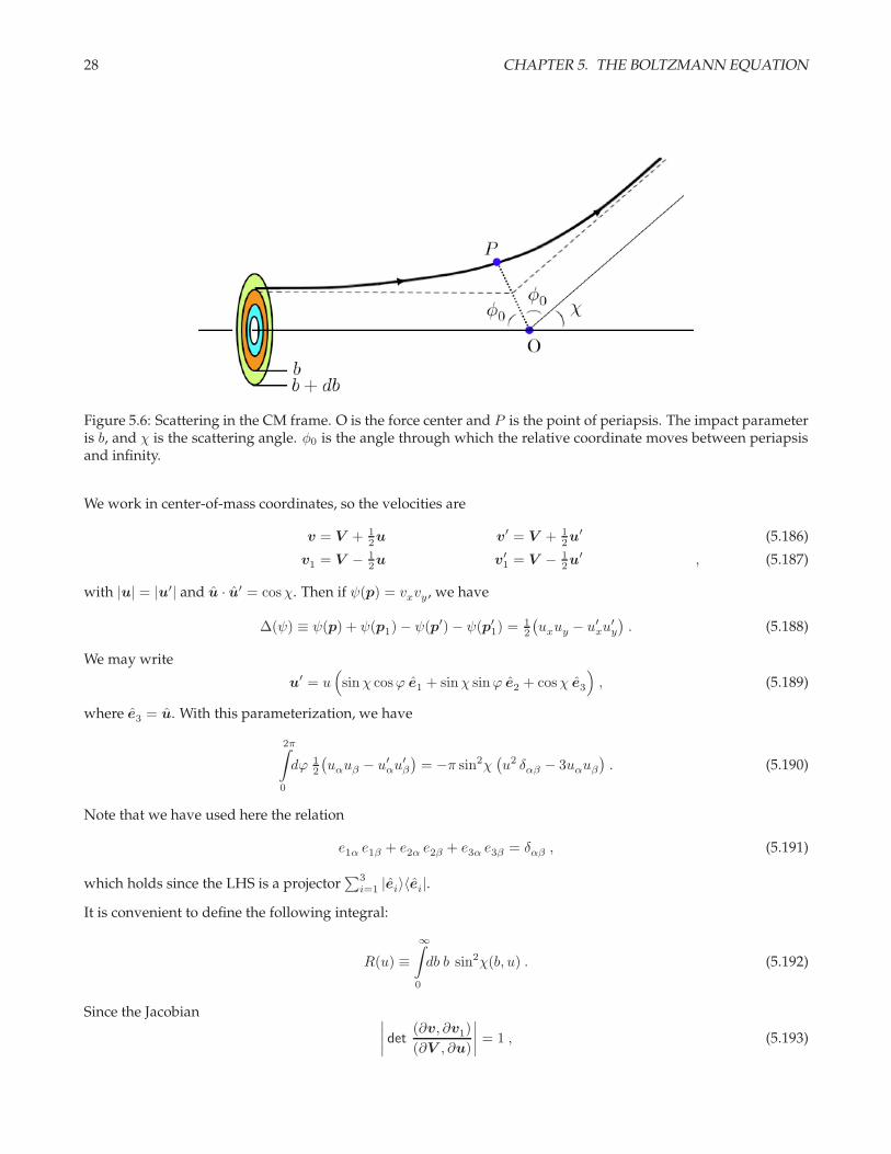
Figure 5.6: Scattering in the CM frame. O is the force center and P is the point of periapsis. The impact parameteris b, and χ is the scattering angle. φ0 is the angle through which the relative coordinate moves between periapsisand infinity.

We work in center-of-mass coordinates, so the velocities are

v = V + 12u v′ = V + 1

2u′ (5.186)

v1 = V − 12u v′

1 = V − 12u′ , (5.187)

with |u| = |u′| and u · u′ = cosχ. Then if ψ(p) = vxvy , we have

∆(ψ) ≡ ψ(p) + ψ(p1) − ψ(p′) − ψ(p′1) = 1

2

(uxuy − u′xu

′y

). (5.188)

We may write

u′ = u(sinχ cosϕ e1 + sinχ sinϕ e2 + cosχ e3

), (5.189)

where e3 = u. With this parameterization, we have

2π∫

0

dϕ 12

(uαuβ − u′αu

′β

)= −π sin2χ

(u2 δαβ − 3uαuβ

). (5.190)

Note that we have used here the relation

e1α e1β + e2α e2β + e3α e3β = δαβ , (5.191)

which holds since the LHS is a projector∑3

i=1 |ei〉〈ei|.

It is convenient to define the following integral:

R(u) ≡∞∫

0

db b sin2χ(b, u) . (5.192)

Since the Jacobian ∣∣∣∣ det(∂v, ∂v1)

(∂V , ∂u)

∣∣∣∣ = 1 , (5.193)


we have

〈 vxvy | L | vxvy 〉 = n2

(m

2πkBT

)3 ∫d3V

∫d3u e−mV 2/kBT e−mu2/4kBT · u · 3π

2 uxuy ·R(u) · vxvy . (5.194)

This yields

〈 vxvy | L | vxvy 〉 = π40 n

2⟨u5R(u)

⟩, (5.195)

where

⟨F (u)

⟩≡

∞∫

0

du u2 e−mu2/4kBT F (u)

/ ∞∫

0

du u2 e−mu2/4kBT . (5.196)

It is easy to compute the term in the numerator of eqn. 5.180:

〈 vxvy | vxvy 〉 = n

(m

2πkBT

)3/2 ∫d3v e−mv2/2kBT v2

x v2y = n

(k

BT

m

)2. (5.197)

Putting it all together, we find

η ≥ 40 (kBT )3

πm2

/⟨u5R(u)

⟩. (5.198)

The computation for κ is a bit more tedious. One has ψ(p) = (ε− cpT ) vx, in which case

∆(ψ) = 12m[(V · u)ux − (V · u′)u′x

]. (5.199)

Ultimately, one obtains the lower bound

κ ≥ 150 kB (kBT )3

πm3

/⟨u5R(u)

⟩. (5.200)

Thus, independent of the potential, this variational calculation yields a Prandtl number of

Pr =ν

a=η cpmκ

= 23 , (5.201)

which is very close to what is observed in dilute monatomic gases (see Tab. 5.1).

While the variational expressions for η and κ are complicated functions of the potential, for hard sphere scatteringthe calculation is simple, because b = d sinφ0 = d cos(1

2χ), where d is the hard sphere diameter. Thus, the impactparameter b is independent of the relative speed u, and one finds R(u) = 1

3d3. Then

⟨u5R(u)

⟩= 1

3d3⟨u5⟩

=128√π

(k

BT

m

)5/2

d2 (5.202)

and one finds

η ≥ 5 (mkBT )1/2

16√π d2

, κ ≥ 75 kB

64√π d2

(kBT

m

)1/2

. (5.203)


5.8 The Equations of Hydrodynamics

We now derive the equations governing fluid flow. The equations of mass and momentum balance are

∂ρ

∂t+ ∇·(ρV ) = 0 (5.204)

∂(ρ Vα)

∂t+∂Παβ

∂xβ= 0 , (5.205)

where

Παβ = ρ VαVβ + p δαβ −

σαβ︷︸︸︷η

(∂Vα

∂xβ

+∂Vβ

∂xα

− 23 ∇·V δαβ

)+ ζ ∇·V δαβ

. (5.206)

Substituting the continuity equation into the momentum balance equation, one arrives at

ρ∂V

∂t+ ρ (V ·∇)V = −∇p+ η∇2V + (ζ + 1

3η)∇(∇·V ) , (5.207)

which, together with continuity, are known as the Navier-Stokes equations. These equations are supplemented byan equation describing the conservation of energy,

T∂s

∂T+ T ∇·(sV ) = σαβ

∂Vα

∂xβ+ ∇·(κ∇T ) . (5.208)

Note that the LHS of eqn. 5.207 is ρDV /Dt, whereD/Dt is the convective derivative. Multiplying by a differentialvolume, this gives the mass times the acceleration of a differential local fluid element. The RHS, multiplied bythe same differential volume, gives the differential force on this fluid element in a frame instantaneously movingwith constant velocity V . Thus, this is Newton’s Second Law for the fluid.

5.9 Nonequilibrium Quantum Transport

5.9.1 Boltzmann equation for quantum systems

Almost everything we have derived thus far can be applied, mutatis mutandis, to quantum systems. The maindifference is that the distribution f0 corresponding to local equilibrium is no longer of the Maxwell-Boltzmannform, but rather of the Bose-Einstein or Fermi-Dirac form,

f0(r,k, t) =

exp

(ε(k) − µ(r, t)

kBT (r, t)

)∓ 1

−1

, (5.209)

where the top sign applies to bosons and the bottom sign to fermions. Here we shift to the more common notationfor quantum systems in which we write the distribution in terms of the wavevector k = p/~ rather than themomentum p. The quantum distributions satisfy detailed balance with respect to the quantum collision integral

(∂f

∂t

)

coll

=

∫d3k1

(2π)3

∫d3k′

(2π)3

∫d3k′1(2π)3

wf ′f ′

1 (1 ± f) (1 ± f1) − ff1 (1 ± f ′) (1 ± f ′1)

(5.210)

where w = w(k,k1 |k′,k′1), f = f(k), f1 = f(k1), f

′ = f(k′), and f ′1 = f(k′

1), and where we have assumedtime-reversal and parity symmetry. Detailed balance requires

f

1 ± f· f11 ± f1

=f ′

1 ± f ′ ·f ′1

1 ± f ′1

, (5.211)

5.9. NONEQUILIBRIUM QUANTUM TRANSPORT 31

where f = f0 is the equilibrium distribution. One can check that

f =1

eβ(ε−µ) ∓ 1=⇒ f

1 ± f= eβ(µ−ε) , (5.212)

which is the Boltzmann distribution, which we have already shown to satisfy detailed balance. For the streamingterm, we have

df0 = kBT∂f0

∂εd

(ε− µ

kBT

)

= kBT∂f0

∂ε

− dµ

kBT− (ε− µ) dT

kBT2

+dε

kBT

= −∂f0

∂ε

∂µ

∂r· dr +

ε− µ

T

∂T

∂r· dr − ∂ε

∂k· dk

,

(5.213)

from which we read off

∂f0

∂r= −∂f

0

∂ε

∂µ

∂r+ε− µ

T

∂T

∂r

∂f0

∂k= ~v

∂f0

∂ε.

(5.214)

The most important application is to the theory of electron transport in metals and semiconductors, in which casef0 is the Fermi distribution. In this case, the quantum collision integral also receives a contribution from one-bodyscattering in the presence of an external potential U(r), which is given by Fermi’s Golden Rule:

(∂f(k)

∂t

)′

coll

=2π

~

∑

k′∈ Ω

|⟨k′∣∣U∣∣k⟩|2(f(k′) − f(k)

)δ(ε(k) − ε(k′)

)

=2π

~V

∫

Ω

d3k

(2π)3| U(k − k′)|2

(f(k′) − f(k)

)δ(ε(k) − ε(k′)

).

(5.215)

The wavevectors are now restricted to the first Brillouin zone, and the dispersion ε(k) is no longer the ballisticform ε = ~

2k2/2m but rather the dispersion for electrons in a particular energy band (typically the valence band)of a solid10. Note that f = f0 satisfies detailed balance with respect to one-body collisions as well11.

In the presence of a weak electric field E and a (not necessarily weak) magnetic field B, we have, within therelaxation time approximation, f = f0 + δf with

∂ δf

∂t− e

~cv × B · ∂ δf

∂k− v ·

[eE+

ε− µ

T∇T

]∂f0

∂ε= −δf

τ, (5.216)

where E = −∇(φ− µ/e) = E − e−1∇µ is the gradient of the ‘electrochemical potential’ φ− e−1µ. In deriving the

above equation, we have worked to lowest order in small quantities. This entails dropping terms like v· ∂ δf∂r (higher

order in spatial derivatives) and E · ∂ δf∂k

(both E and δf are assumed small). Typically τ is energy-dependent, i.e.

τ = τ(ε(k)

).

10We neglect interband scattering here, which can be important in practical applications, but which is beyond the scope of these notes.11The transition rate from |k′〉 to |k〉 is proportional to the matrix element and to the product f ′(1− f). The reverse process is proportional

to f(1 − f ′). Subtracting these factors, one obtains f ′ − f , and therefore the nonlinear terms felicitously cancel in eqn. 5.215.


We can use eqn. 5.216 to compute the electrical current j and the thermal current jq ,

j = −2e

∫

Ω

d3k

(2π)3v δf (5.217)

jq = 2

∫

Ω

d3k

(2π)3(ε− µ)v δf . (5.218)

Here the factor of 2 is from spin degeneracy of the electrons (we neglect Zeeman splitting).

In the presence of a time-independent temperature gradient and electric field, linearized Boltzmann equation inthe relaxation time approximation has the solution

δf = −τ(ε)v ·(eE+

ε− µ

T∇T

)(−∂f

0

∂ε

). (5.219)

We now consider both the electrical current12 j as well as the thermal current density jq . One readily obtains

j = −2e

∫

Ω

d3k

(2π)3v δf ≡ L11 E− L12 ∇T (5.220)

jq = 2

∫

Ω

d3k

(2π)3(ε− µ)v δf ≡ L21 E− L22 ∇T (5.221)

where the transport coefficients L11 etc. are matrices:

Lαβ11 =

e2

4π3~

∫dε τ(ε)

(−∂f

0

∂ε

)∫dSε

vα vβ

|v| (5.222)

Lαβ21 = TLαβ

12 = − e

4π3~

∫dε τ(ε) (ε− µ)

(−∂f

0

∂ε

)∫dSε

vα vβ

|v| (5.223)

Lαβ22 =

1

4π3~T

∫dε τ(ε) (ε− µ)2

(−∂f

0

∂ε

)∫dSε

vα vβ

|v| . (5.224)

If we define the hierarchy of integral expressions

J αβn ≡ 1

4π3~

∫dε τ(ε) (ε− µ)n

(−∂f

0

∂ε

)∫dSε

vα vβ

|v| (5.225)

then we may write

Lαβ11 = e2J αβ

0 , Lαβ21 = TLαβ

12 = −eJ αβ1 , Lαβ

22 =1

TJ αβ

2 . (5.226)

The linear relations in eqn. (5.221) may be recast in the following form:

E = ρ j +Q∇T

jq = ⊓ j − κ∇T ,(5.227)

where the matrices ρ, Q, ⊓, and κ are given by

ρ = L−111 Q = L−1

11 L12 (5.228)

⊓ = L21 L−111 κ = L22 − L21L

−111 L12 , (5.229)

12In this section we use j to denote electrical current, rather than particle number current as before.


Figure 5.7: A thermocouple is a junction formed of two dissimilar metals. With no electrical current passing, anelectric field is generated in the presence of a temperature gradient, resulting in a voltage V = VA − VB.

or, in terms of the Jn,

ρ =1

e2J −1

0 Q = − 1

e TJ −1

0 J1 (5.230)

⊓ = −1

eJ1 J −1

0 κ =1

T

(J2 − J1 J −1

0 J1

), (5.231)

These equations describe a wealth of transport phenomena:

• Electrical resistance (∇T = B = 0)An electrical current j will generate an electric field E = ρj, where ρ is the electrical resistivity.

• Peltier effect (∇T = B = 0)An electrical current j will generate an heat current jq = ⊓j, where ⊓ is the Peltier coefficient.

• Thermal conduction (j = B = 0)A temperature gradient ∇T gives rise to a heat current jq = −κ∇T , where κ is the thermal conductivity.

• Seebeck effect (j = B = 0)A temperature gradient ∇T gives rise to an electric field E = Q∇T , where Q is the Seebeck coefficient.

One practical way to measure the thermopower is to form a junction between two dissimilar metals, A and B. Thejunction is held at temperature T1 and the other ends of the metals are held at temperature T0. One then measuresa voltage difference between the free ends of the metals – this is known as the Seebeck effect. Integrating theelectric field from the free end of A to the free end of B gives

VA − VB = −B∫

A

E · dl = (QB −QA)(T1 − T0) . (5.232)

What one measures here is really the difference in thermopowers of the two metals. For an absolute measurementof QA, replace B by a superconductor (Q = 0 for a superconductor). A device which converts a temperaturegradient into an emf is known as a thermocouple.


Figure 5.8: A sketch of a Peltier effect refrigerator. An electrical current I is passed through a junction betweentwo dissimilar metals. If the dotted line represents the boundary of a thermally well-insulated body, then the bodycools when ⊓B > ⊓A, in order to maintain a heat current balance at the junction.

The Peltier effect has practical applications in refrigeration technology. Suppose an electrical current I is passedthrough a junction between two dissimilar metals, A and B. Due to the difference in Peltier coefficients, there willbe a net heat current into the junction of W = (⊓A − ⊓B) I . Note that this is proportional to I , rather than thefamiliar I2 result from Joule heating. The sign of W depends on the direction of the current. If a second junctionis added, to make an ABA configuration, then heat absorbed at the first junction will be liberated at the second. 13

5.9.2 The Heat Equation

We begin with the continuity equations for charge density ρ and energy density ε:

∂ρ

∂t+ ∇ · j = 0 (5.233)

∂ε

∂t+ ∇ · jε = j ·E , (5.234)

where E is the electric field14. Now we invoke local thermodynamic equilibrium and write

∂ε

∂t=∂ε

∂n

∂n

∂t+∂ε

∂T

∂T

∂t

= −µe

∂ρ

∂t+ cV

∂T

∂t, (5.235)

13To create a refrigerator, stick the cold junction inside a thermally insulated box and the hot junction outside the box.14Note that it is E · j and not E · j which is the source term in the energy continuity equation.


where n is the electron number density (n = −ρ/e) and cV is the specific heat. We may now write

cV∂T

∂t=∂ε

∂t+µ

e

∂ρ

∂t

= j · E − ∇ · jε −µ

e∇ · j

= j · E− ∇ · jq . (5.236)

Invoking jq = ⊓j − κ∇T , we see that if there is no electrical current (j = 0), we obtain the heat equation

cV∂T

∂t= καβ

∂2T

∂xα ∂xβ. (5.237)

This results in a time scale τT for temperature diffusion τT = CL2cV /κ, where L is a typical length scale and C isa numerical constant. For a cube of size L subjected to a sudden external temperature change, L is the side lengthand C = 1/3π2 (solve by separation of variables).

5.9.3 Calculation of Transport Coefficients

We will henceforth assume that sufficient crystalline symmetry exists (e.g. cubic symmetry) to render all the trans-port coefficients multiples of the identity matrix. Under such conditions, we may write J αβ

n = Jn δαβ with

Jn =1

12π3~

∫dε τ(ε) (ε− µ)n

(−∂f

0

∂ε

)∫dSε |v| . (5.238)

The low-temperature behavior is extracted using the Sommerfeld expansion,

I ≡∞∫

−∞

dεH(ε)

(−∂f

0

∂ε

)= πD csc(πD)H(ε)

∣∣∣ε=µ

(5.239)

= H(µ) +π2

6(kBT )2H ′′(µ) + . . . (5.240)

where D ≡ kBT ∂

∂ε is a dimensionless differential operator.15

Let us now perform some explicit calculations in the case of a parabolic band with an energy-independent scat-tering time τ . In this case, one readily finds

Jn =σ0

e2µ−3/2 πD cscπD ε3/2 (ε− µ)n

∣∣∣ε=µ

, (5.241)

where σ0 = ne2τ/m∗. Thus,

J0 =σ0

e2

[1 +

π2

8

(kBT )2

µ2+ . . .

]

J1 =σ0

e2π2

2

(kBT )2

µ+ . . .

J2 =σ0

e2π2

3(k

BT )2 + . . . ,

(5.242)

15Remember that physically the fixed quantities are temperature and total carrier number density (or charge density, in the case of electronand hole bands), and not temperature and chemical potential. An equation of state relating n, µ, and T is then inverted to obtain µ(n, T ), sothat all results ultimately may be expressed in terms of n and T .


from which we obtain the low-T results ρ = σ−10 ,

Q = −π2

2

k2BT

e εFκ =

π2

3

nτ

m∗ k2BT , (5.243)

and of course ⊓ = TQ. The predicted universal ratio

κ

σT=π2

3(kB/e)

2 = 2.45 × 10−8 V2 K−2 , (5.244)

is known as the Wiedemann-Franz law. Note also that our result for the thermopower is unambiguously nega-tive. In actuality, several nearly free electron metals have positive low-temperature thermopowers (Cs and Li, forexample). What went wrong? We have neglected electron-phonon scattering!

5.9.4 Onsager Relations

Transport phenomena are described in general by a set of linear relations,

Ji = Lik Fk , (5.245)

where the Fk are generalized forces and the Ji are generalized currents. Moreover, to each force Fi corresponds aunique conjugate current Ji, such that the rate of internal entropy production is

S =∑

i

Fi Ji =⇒ Fi =∂S

∂Ji. (5.246)

The Onsager relations (also known as Onsager reciprocity) state that

Lik(B) = ηi ηk Lki(−B) , (5.247)

where ηi describes the parity of Ji under time reversal:

JTi = ηi Ji , (5.248)

where JTi is the time reverse of Ji. To justify the Onsager relations requires a microscopic description of our

nonequilibrium system.

The Onsager relations have some remarkable consequences. For example, they require, for B = 0, that the thermal

conductivity tensor κij of any crystal must be symmetric, independent of the crystal structure. In general,thisresult does not follow from considerations of crystalline symmetry. It also requires that for every ‘off-diagonal’transport phenomenon, e.g. the Seebeck effect, there exists a distinct corresponding phenomenon, e.g. the Peltiereffect.

For the transport coefficients studied, Onsager reciprocity means that in the presence of an external magnetic field,

ραβ(B) = ρβα(−B) (5.249)

καβ(B) = κβα(−B) (5.250)

⊓αβ(B) = T Qβα(−B) . (5.251)

Let’s consider an isotropic system in a weak magnetic field, and expand the transport coefficients to first order inB:

ραβ(B) = ρ δαβ + ν ǫαβγ Bγ (5.252)

καβ(B) = κ δαβ + ǫαβγ Bγ (5.253)

Qαβ(B) = Qδαβ + ζ ǫαβγ Bγ (5.254)

⊓αβ(B) = ⊓ δαβ + θ ǫαβγBγ . (5.255)

5.10. APPENDIX : BOLTZMANN EQUATION AND COLLISIONAL INVARIANTS 37

Onsager reciprocity requires ⊓ = T Q and θ = T ζ. We can now write

E = ρ j + ν j × B +Q∇T + ζ∇T × B (5.256)

jq = ⊓ j + θ j × B − κ∇T −∇T × B . (5.257)

There are several new phenomena lurking:

• Hall effect ( ∂T∂x = ∂T

∂y = jy = 0)

An electrical current j = jx x and a field B = Bz z yield an electric field E. The Hall coefficient is RH =Ey/jxBz = −ν.

• Ettingshausen effect ( ∂T∂x = jy = jq,y = 0)

An electrical current j = jx x and a field B = Bz z yield a temperature gradient ∂T∂y . The Ettingshausen

coefficient is P = ∂T∂y

/jxBz = −θ/κ.

• Nernst effect (jx = jy = ∂T∂y = 0)

A temperature gradient ∇T = ∂T∂x x and a field B = Bz z yield an electric field E. The Nernst coefficient is

Λ = Ey

/∂T∂x Bz = −ζ.

• Righi-Leduc effect (jx = jy = Ey = 0)

A temperature gradient ∇T = ∂T∂x x and a field B = Bz z yield an orthogonal temperature gradient ∂T

∂y .

The Righi-Leduc coefficient is L = ∂T∂y

/∂T∂xBz = ζ/Q.

5.10 Appendix : Boltzmann Equation and Collisional Invariants

Problem : The linearized Boltzmann operator Lψ is a complicated functional. Suppose we replace L by L, where

Lψ = −γ ψ(v, t) + γ

(m

2πkBT

)3/2 ∫d3u exp

(− mu2

2kBT

)

×

1 +m

kBTu · v +

2

3

(mu2

2kBT− 3

2

)(mv2

2kBT− 3

2

)ψ(u, t) .

(5.258)

Show that L shares all the important properties of L. What is the meaning of γ? Expand ψ(v, t) in sphericalharmonics and Sonine polynomials,

ψ(v, t) =∑

rℓm

arℓm(t)Sr

ℓ+12

(x)xℓ/2 Y ℓm(n), (5.259)

with x = mv2/2kBT , and thus express the action of the linearized Boltzmann operator algebraically on the expan-sion coefficients arℓm(t).

The Sonine polynomials Snα(x) are a complete, orthogonal set which are convenient to use in the calculation of

transport coefficients. They are defined as

Snα(x) =

n∑

m=0

Γ(α + n+ 1) (−x)m

Γ(α+m+ 1) (n−m)!m!, (5.260)


and satisfy the generalized orthogonality relation

∞∫

0

dx e−x xα Snα(x)Sn′

α (x) =Γ(α+ n+ 1)

n!δnn′ . (5.261)

Solution : The ‘important properties’ of L are that it annihilate the five collisional invariants, i.e. 1, v, and v2, andthat all other eigenvalues are negative. That this is true for L can be verified by an explicit calculation.

Plugging the conveniently parameterized form of ψ(v, t) into L, we have

Lψ = −γ∑

rℓm

arℓm(t) Sr

ℓ+12

(x) xℓ/2 Y ℓm(n) +

γ

2π3/2

∑

rℓm

arℓm(t)

∞∫

0

dx1 x1/21 e−x1

×∫dn1

[1 + 2 x1/2x

1/21 n·n1 + 2

3

(x− 3

2

)(x1 − 3

2

)]Sr

ℓ+12

(x1) xℓ/21 Y ℓ

m(n1) ,

(5.262)

where we’ve used

u =

√2kBT

mx

1/21 , du =

√kBT

2mx−1/21 dx1 . (5.263)

Now recall Y 00 (n) = 1√

4πand

Y 11 (n) = −

√3

8πsin θ eiϕ Y 1

0 (n) =

√3

4πcos θ Y 1

−1(n) = +

√3

8πsin θ e−iϕ

S01/2(x) = 1 S0

3/2(x) = 1 S11/2(x) = 3

2 − x ,

which allows us to write

1 = 4π Y 00 (n)Y 0

0∗(n1) (5.264)

n·n1 =4π

3

[Y 1

0 (n)Y 10∗(n1) + Y 1

1 (n)Y 11∗(n1) + Y 1

−1(n)Y 1−1

∗(n1)

]. (5.265)

We can do the integrals by appealing to the orthogonality relations for the spherical harmonics and Sonine poly-nomials:

∫dnY ℓ

m(n)Y l′

m′

∗(n) = δll′ δmm′ (5.266)

∞∫

0

dx e−x xα Snα(x)Sn′

α (x) =Γ(n+ α+ 1)

Γ(n+ 1)δnn′ . (5.267)

5.10. APPENDIX : BOLTZMANN EQUATION AND COLLISIONAL INVARIANTS 39

Integrating first over the direction vector n1,

Lψ = −γ∑

rℓm

arℓm(t) Sr

ℓ+12

(x) xℓ/2 Y ℓm(n)

+2γ√π

∑

rℓm

arℓm(t)

∞∫

0

dx1 x1/21 e−x1

∫dn1

[Y 0

0 (n)Y 00∗(n1)S

01/2(x)S

01/2(x1)

+ 23 x

1/2x1/21

1∑

m′=−1

Y 1m′(n)Y 1

m′

∗(n1)S

03/2(x)S

03/2(x1)

+ 23 Y

00 (n)Y 0

0∗(n1)S

11/2(x)S

11/2(x1)

]Sr

ℓ+12

(x1) xℓ/21 Y ℓ

m(n1) ,

(5.268)

we obtain the intermediate result

Lψ = −γ∑

rℓm

arℓm(t) Sr

ℓ+12

(x) xℓ/2 Y ℓm(n)

+2γ√π

∑

rℓm

arℓm(t)

∞∫

0

dx1 x1/21 e−x1

[Y 0

0 (n) δl0 δm0 S01/2(x)S

01/2(x1)

+ 23 x

1/2x1/21

1∑

m′=−1

Y 1m′(n) δl1 δmm′ S0

3/2(x)S03/2(x1)

+ 23 Y

00 (n) δl0 δm0 S

11/2(x)S

11/2(x1)

]Sr

ℓ+12

(x1) x1/21 .

(5.269)

Appealing now to the orthogonality of the Sonine polynomials, and recalling that

Γ(12 ) =

√π , Γ(1) = 1 , Γ(z + 1) = z Γ(z) , (5.270)

we integrate over x1. For the first term in brackets, we invoke the orthogonality relation with n = 0 and α = 12 ,

giving Γ(32 ) = 1

2

√π. For the second bracketed term, we have n = 0 but α = 3

2 , and we obtain Γ(52 ) = 3

2 Γ(32 ),

while the third bracketed term involves leads to n = 1 and α = 12 , also yielding Γ(5

2 ) = 32 Γ(3

2 ). Thus, we obtainthe simple and pleasing result

Lψ = −γ∑

rℓm

′arℓm(t) Sr

ℓ+12

(x) xℓ/2 Y ℓm(n) (5.271)

where the prime on the sum indicates that the set

CI =(0, 0, 0) , (1, 0, 0) , (0, 1, 1) , (0, 1, 0) , (0, 1,−1)

(5.272)

are to be excluded from the sum. But these are just the functions which correspond to the five collisional invariants!Thus, we learn that

ψrℓm(v) = Nrℓm Sr

ℓ+12

(x)xℓ/2 Y ℓm(n), (5.273)

is an eigenfunction of L with eigenvalue −γ if (r, ℓ,m) does not correspond to one of the five collisional invariants.In the latter case, the eigenvalue is zero. Thus, the algebraic action of L on the coefficients arℓm is

(La)rℓm =

−γ arℓm if (r, ℓ,m) /∈ CI

= 0 if (r, ℓ,m) ∈ CI(5.274)


The quantity τ = γ−1 is the relaxation time.

It is pretty obvious that L is self-adjoint, since

〈φ | Lψ 〉 ≡∫d3v f0(v)φ(v)L[ψ(v)]

= −γ n(

m

2πkBT

)3/2∫d3v exp

(− mv2

2kBT

)φ(v)ψ(v)

+ γ n

(m

2πkBT

)3 ∫d3v

∫d3u exp

(− mu2

2kBT

)exp

(− mv2

2kBT

)

× φ(v)

[1 +

m

kBTu · v +

2

3

(mu2

2kBT− 3

2

)(mv2

2kBT− 3

2

)]ψ(u)

= 〈 Lφ |ψ 〉 ,

(5.275)

where n is the bulk number density and f0(v) is the Maxwellian velocity distribution.

contentsphysics.ucsd.edu/.../courses/fall2013/physics210b/lectures/ch05.pdf · contents 5 the...

Documents