brics · brics rs-00-37 hune et al.: ... which is a case study of the vhs project1. ... to meet...

BR

ICS

RS

-00-37H

uneetal.:

Guided

Synthesis

ofControlP

rograms

fora

Batch

Plantusing

UPPA

AL

BRICSBasic Research in Computer Science

Guided Synthesis of Control Programs fora Batch Plant using UPPAAL

Thomas S. HuneKim G. LarsenPaul Pettersson

BRICS Report Series RS-00-37

ISSN 0909-0878 December 2000

Copyright c© 2000, Thomas S. Hune & Kim G. Larsen & PaulPettersson.BRICS, Department of Computer ScienceUniversity of Aarhus. All rights reserved.

Reproduction of all or part of this workis permitted for educational or research useon condition that this copyright notice isincluded in any copy.

See back inner page for a list of recent BRICS Report Series publications.Copies may be obtained by contacting:

BRICSDepartment of Computer ScienceUniversity of AarhusNy Munkegade, building 540DK–8000 Aarhus CDenmarkTelephone: +45 8942 3360Telefax: +45 8942 3255Internet: [email protected]

BRICS publications are in general accessible through the World WideWeb and anonymous FTP through these URLs:

http://www.brics.dkftp://ftp.brics.dkThis document in subdirectory RS/00/37/

Guided Synthesis of Control Programs

for a Batch Plant using Uppaal?

Thomas Hune1, Kim G. Larsen2, and Paul Pettersson3

1 BRICS†, University of Arhus, Denmark,Email: [email protected]

2 BRICS†, University of Aalborg, Denmark,Email: [email protected]

3 Department of Computer Systems, Information Technology,Uppsala University, E-mail: [email protected].

Abstract. In this paper we address the problem of scheduling and syn-thesizing distributed control programs for a batch production plant. Weuse a timed automata model of the batch plant and the verification toolUppaal to solve the scheduling problem.In modeling the plant, we aim at a level of abstraction which is suffi-ciently accurate in order that synthesis of control programs from gener-ated timed traces is possible. Consequently, the models quickly becometoo detailed and complicated for immediate automatic synthesis. In fact,only models of plants producing two batches can be analyzed directly! Toovercome this problem, we present a general method allowing the user toguide the model-checker according to heuristically chosen strategies. Theguidance is specified by augmenting the model with additional guidancevariables and by decorating transitions with extra guards on these. Ap-plying this method have made synthesis of control programs feasible fora plant producing as many as 60 batches.The synthesized control programs have been executed in a physical plant.Besides proving useful in validating the plant model and in finding somemodeling errors, we view this final step as the ultimate litmus test of ourmethodology’s ability to generate executable (and executing) code frombasic plant models.

1 Introduction

In this paper we suggest a solution to the problem of synthesizing andverifying valid scheduling control programs for resource allocation,

? This work is partially supported by the European Community Esprit-LTR Project26270 VHS (Verification of Hybrid systems).

† Basic Research In Computer Science, Centre of the Danish National ResearchFoundation.

based on a batch plant of SIDMAR [BS99,Feh99], which is a casestudy of the VHS project1. We model the plant in a network of timedautomata, with the different components of the plant (e.g. batches,recipes, casting machine, cranes, etc.) constituting the individualtimed automata. The scheduling problem is formulated as a time-bounded reachability question allowing us to apply the real-timemodel-checking tool Uppaal [LPY95,LPY97] to derive a schedule.An overview of the methodology is shown in Figure 1.

Uppaal offers a trace with actions of the model and timing infor-mation of the actions. The remaining effort required in transform-ing such a model trace into an executable control program dependsheavily on the accuracy of the model with respect to the controlprogramming language and the physical properties of the plant. Inthe Uppaal model given in [Feh99], movement along tracks and onthe cranes was assumed to be instantaneous. Making a schedule con-taining timing information from a trace like that is very hard, andsometimes it is not possible at all. However, given a sufficiently highlevel of accuracy of the plant model, a schedule can be obtained froma trace by projection, and synthesis of the control program from aschedule amounts to textual substitution. Unfortunately model suit-able for such program synthesis becomes very detailed as all thenecessary information about the plant, such as the timing boundsand the physical constraints for movements of loads, cranes etc, havebe to specified. As an immediate drawback, synthesizing schedulesfor several batches quickly becomes infeasible. Even for the moreabstract models presented in [Feh99] this problem was also encoun-tered.

To deal with this (unavoidable) problem we introduce a method,allowing the user to guide the model-checking according to certainchosen strategies. Each strategy will contribute with a reduction ofthe search-space, but in contrast to fully automatic reduction meth-ods like partial order reduction [BJLY98] it is up to the user to’guarantee’ preservation of schedulability. However, if a schedule isidentified via the guided search, the schedule is indeed a valid one forthe original model. Since we are not interested in optimal schedulesthis is sufficient.1 See the web site http://www-verimag.imag.fr//VHS/main.html.

2

Plant Model

SIDMAR Plant

Schedule

LEGO Plant

Guided Plant Model

Control Program

desired realized

Fig. 1. Overview of methodology.

To be able to run the generated control programs in a physical plant,we consider a LEGO MINDSTORMS plant, instead of the orig-inal plant of SIDMAR. We have used the plant to successfully runsynthesized control programs and by doing so increased our confi-dence in the plant model. We view this final, scientifically rathersimple, step as the ultimate litmus test of our methodology’s abil-ity to generate executable (and executing) code from rather naturalplant models.

The SIDMAR plant has been studied by several other researchers.Our timed automata model is based on the model in [Feh99], whichis similar to ours but more abstract in the sense that some infor-mation, such as delays for the moving of batches, is not included.A Petri net model of the plant is presented in [BS99]. In [Sto00],constraint programming techniques are used to generate schedulesof the SIDMAR plant for up to 30 batches. This result is achievedby reducing the size of the plant model using techniques similar tothe guiding techniques presented in this paper. Other work apply-ing the model of timed automata and Uppaal to analyze and solveplanning problems of batch plants include [KLPW99] in which anexperimental batch plant is studied.

The rest of this paper is organized as follows: In the next two sectionswe describe the scheduling problem and how it has been modeled in

3

Uppaal. In Section 4 and 5 we present the guiding techniques andevaluate their effect on the plant model. In Section 6 we describeexperiments with the LEGO plant and how programs are synthe-sized for the plant. Section 7 concludes the paper. Finally, timedautomata descriptions of four plant components are enclosed in theappendix.

2 The Scheduling Problem

Our plant is based on a part of the SIDMAR steel production plantlocated at Gent in Belgium. We will consider the part of the plantbetween the blast furnace and the continuous casting machine wheremolten pig iron is converted into steel of different qualities. Theprocess is started when pig iron being poured into ladles by one oftwo converter vessels. The iron is transported in the ladles whileit is being processed. By treatments in different machines the ironis converted into steel and finally casted in the casting machine.Depending on the machines used and how long the treatment inthe machines last, different qualities of steel are produced. Whenthe steel in a ladle has been casted the empty ladle must be movedto a storage place. From here the ladles are cleaned and reused.However, this is not part of our model, where ladles are stored atthe storage place but not reused. The physical components of theprocess are: two converter vessels where molten iron is poured intoladles, five machines, tracks connecting these, two cranes running onone overhead track, a buffer place, a storage place for empty ladles,and one casting machine. The layout of the plant can be seen inFigure 2.

Machines number one and four are of the same type and so aremachines number two and five. Each crane can only hold one ladleand they cannot overtake each other. On each track and in eachmachine there is room for at most one ladle. This means that theladles cannot overtake each other without using one of the cranes.

The steel must sustain a minimum temperature during the process.This gives an upper bound on the time a batch is allowed to spendin the plant from it is poured and until it is casted. Casting takes a

4

��

��

��

��

��

��

��

��

continuous

machinecasting

place

storage

holding

place

convertorvessel #2

machine#1

track#2

machine#2 machine#3

overheadcranes

machine#4 machine#5

track#1

crane#2

crane#1

buffer

convertorvessel #1

Fig. 2. Layout of the plant.

fixed time and must be continuous. Therefore a new ladle filled withsteel must be waiting in the holding place of the casting machinewhen casting of a ladle has finished.

Steel of different qualities can be produced depending on which typesof machines are visited and for how long. For each batch this isspecified by a recipe. The problem to be solved can now be statedas:

Given an ordered list of recipes, if possible synthesize a controlprogram for the plant such that steel specified by the recipes areproduced in the right order and within a given time.

The major part of solving this problem is finding a schedule for theproduction if one exists. A schedule for the plant defines which actiontakes place in the plant e.g. moving of batches and cranes, and whenthe actions take place.

3 Scheduling with Timed Automata

Finding a schedule for producing an ordered list of steel qualities isthe main part of the problem. It can be solved in a number of ways.

5

S0x<=4

S1x<=5,y<=3

S2

P: Q:x>=1, j<50 y:=0, j:=j+2

x:=0, y:=0 a!

i<10

i:=i+1a?

Fig. 3. A Network of Timed Automata.

Here we chose to model the plant using timed automata [AD94]and use the verification tool Uppaal [LPY95,LPY97] to solve thescheduling problem 2. The use of timed automata for modeling theplant allows the scheduling problem to be reformulated as a reacha-bility problem which can be solved by Uppaal. A discussion of thisapproach to scheduling can be found in [Feh99].

The modeling language in Uppaal is networks of timed automataextended with data variables [LPY97]. To meet requirements fromvarious case-studies the language has been further extended with thenotion of committed locations [BGK+96], urgent synchronization ac-tions [LPY97], and data structures such as arrays of data-variablesetc. In this section we give a brief informal description of the mod-eling language of Uppaal. For a detailed description we refer thereader to [LPY97].

3.1 Networks of Timed Automata

Consider the network of timed automata P and Q shown in Fig-ure 3.1. Automaton P has two control locations S0 and S1, tworeal-valued clocks x and y, and a data variable j. A state of theautomaton is of the form (l, s, t, k), where l is a control location, sand t are non-negative reals giving the value of the two clocks x andy, and k is a natural number giving value to the data variable j.A control location is labelled with a condition (the location invari-ant) on the clock values that must be satisfied for states involvingthis location. Assuming that the automaton starts to operate in the

2 See the web site http://www.uppaal.com/ for more information about Uppaal.

6

state (S0, 0, 0, 0), it may stay in location S0 as long as the invari-ant x ≤ 4 of S0 is satisfied. During this time the values of theclocks increase synchronously. Thus from the initial state, all statesof the form (S0, t, t, 0), where t ≤ 4, are reachable. The edges of atimed automaton may be decorated with a condition (guard) on theclocks and the data variable values that must be satisfied in order forthe edge to be enabled. Thus, only for the states (S0, t, t, k), where1 ≤ t ≤ 4 and k < 50, is the edge from S0 to S1 enabled. Addition-ally, edges may be labelled with assignments and synchronizationlabels. An assignment may reset the value of the clocks and updatethe data variables. For example, when following the edge from S0 toS1 the clock y is reset to 0 and the data variable j is incrementedby 2, leading to states of the form (S1, t, 0, 2), where 1 ≤ t ≤ 4. Thesynchronization label is used to establish synchronization betweenautomata. For example the transition from S1 to S0 of automatonP is labeled with a!, requiring the transition to be synchronized withthe transition of automaton Q offering the complementary action a?.

In general, a timed automaton is a finite-state automata extendedwith a finite collection C of real-valued clocks ranged over by x, yetc. and a finite set of data variables D ranged over by i, j etc. Weuse B(C) ranged over by g to stand for the set of formulas that canbe an atomic constraint of the form: x ∼ n or x− y ∼ n for x, y ∈ C,∼∈{<,≤, =,≥>} and n being a natural number, or a conjunctionof such formulas. Similarly, we use B(D) to stand for the set of data-variable constraints that are the conjunctive formulas of i ∼ j ori ∼ k, where ∼ ∈ {<,≤, =, 6=,≥, >} and k is an integer number. Todenote the set of formulas that are conjunctions of clock constraintsand a data-variable constraints we use B(C,D) (ranged over by g).The elements of B(C,D) are called constraints or guards.

An assignment in Uppaal is a sequence of operations of the formx :=0, or i :=Expr, where x is a clock, i is a data variable, and Expris an integer expression, e.g. 2∗(i−j)+3 (where j is a data variable).We shall use R to denote the set of assignments. Furthermore, weuse Act to denote a finite set of actions ranged over by a, a?, a!, b?,b!, etc.

7

Definition 1 (Timed Automata). A timed automaton A overclocks C and data variables D is a tuple 〈N, l0,−→, I〉 where N isa finite set of (control-)locations, l0 is the initial location, −→⊆N × B(C,D) × Act × R × N corresponds to the set of edges andfinally, I : N 7→ B(C) assigns invariants to locations. In the case,

〈l, g, a, r, l′〉 ∈−→, we write lg,a,r−→ l′. ut

To formalize the semantics we use variable assignments. A variableassignment is a mapping which maps the clocks C to the non-negativereals and the data variables D to integers. A semantical state of anautomaton A is now a tuple (l, u), where l is a location of A andu is a an assignment for C and D, and the semantics of A is givenby a transition system with the following two types of transitions(corresponding to delay-transitions and action-transitions):

– (l, u) −→ (l, u ⊕ d) if I(l)(u) and I(l)(u ⊕ d)

– (l, u) −→ (l′, u′) if there exist g and r such that lg,a,r−→ l′, g(u),

u′ = r[u], and I(l′)(u′)

where d is a non-negative real number, u⊕d denotes the assignmentwhich maps each clock x in C to the value u(x) + d and leaves eachdata variable i with the unchanged value u(i), and r[u] denotes theresult of updating the clocks C and the data-variables in D accordingto r ∈ R.

Finally, we briefly introduce the notion of networks of timed au-tomata [YPD94,LPY95]. A network is a finite set of automata com-posed in parallel with a CCS-like parallel composition operator [Mil89].For a network with the timed automata A1, . . . , An the intuitivemeaning is similar to the CCS parallel composition of A1, ..., An withall actions being restricted, that is, (A1|...|An)\Act. Thus an edgelabelled with action a must synchronize with an edge labelled withan action complementary to a, and edges with the silent τ action areinternal, so they do not synchronize. In Uppaal ’?’ and ’ !’ are usedto represent complementary actions, so a? and a! are consideredcomplementary and can synchronize.

8

3.2 Analysis

Given a network of timed automata and a set of states, Uppaal cananalyze whether or not one of the states is reachable from the initialstate of the network. If the answer is positive, Uppaal producesa trace with action- and delays-transitions leading from the initialstate to one of the specified states.

For the model of the plant, which will be presented in the follow-ing, a trace defines a schedule for the plant since it specifies whathappens in the plant (the synchronization actions) and when (thedelays). From a schedule a working program controlling the plantmay be generated. The level of detail in the trace (and therefore inthe schedule) influences the work needed to generate the program.In [Feh99] the traces generated did not include time for the movingof batches, making the generation of executable programs from theschedules hard. To minimize the effort needed during the transla-tion, we produce traces with detailed and precise information abouttiming of all actions in the plant.

3.3 A Model for Scheduling the Plant

An instance of the problem is given by a list of qualities of steel(or recipes) and a maximal production time. A model of a prob-lem instance consists of: for each recipe one automaton representingthe recipe and one automaton representing the movement of thebatch; one automaton for each of the two cranes; one automatontesting that the recipes finish in the correct order; one automatonfor making some actions synchronizing; and one automaton modelingthe casting machine. Figure 4 shows the synchronizations betweenthe different automata. The batch automata communicate with eachother through two shared arrays and the two cranes also share anarray. These arrays will be described in more detail later.

The most complex of the automata is the one modeling the possiblebehaviors of a batch (see Figure 16 of the appendix3)4. The batch3 Unless stated otherwise, guided versions of the automata are shown since these have

been used for most of the experiments.4 Pictures of all the automata and the LEGO plant can be found at the web sitehttp://www.brics.dk/~baris/CaseStudy/.

9

Recipe 3

Recipe n

Tester

Batch 1

Controller Crane A Crane BMachineCasting

Recipe 2

Recipe 1

Batch 2

Batch 3

Batch n

Fig. 4. Synchronization between the automata of a model.

automaton reflects the topology of the plant (shown in Figure 2) aswell as the physical constraints on the movements of a batch. Ba-sically, there is one location for each position of the plant a batchcan be located at. A position is either a machine, a track segment,the storage place, the casting machine, or a position on the overheadtrack. Positions on the overhead track are over one of the two tracks,the storage place, the casting machine, or in between any of these. Abatch automaton has a clock named x associated to it which is usedto measure the time spend on moving along a track. The time spendis the worst case time measured in the physical plant which is givenby the constant bmove. Shared among all the batch automata in amodel are the two binary arrays posI and posII, which are used forstoring which positions are occupied on the two tracks. These areused to ensure that each position is occupied by at most one batchat a time. Figure 5 shows the part of the unguided batch automatonmodeling the position named i2, between machines number one andtwo on track one. Moving a batch between positions in the modelis done in two steps. First a transition is taken to an intermediate

10

i1a

x<=bmove

i2 i2a

x<=bmove

k1

i1aax<=bmove

i2aax<=bmove

c1down

i1

x==bmove,posI[4]==0

posI[4]:=1,posI[3]:=0

posI[5]==0

posI[5]:=1,posI[4]:=0,x:=0

b2right?

cAIup!

posI[3]==0

posI[3]:=1,posI[4]:=0,x:=0

b2left?x==bmove,posI[4]==0

posI[4]:=1,posI[5]:=0

cIdown_end?cBIup!

posI[3]==0

posI[3]:=1,posI[2]:=0,x:=0

m1right?

x==bmove,posI[2]==0

posI[2]:=0,posI[3]:=0

Fig. 5. Part of the unguided batch automaton.

position, e.g. from i2 to i1aa. A batch can only start to move toa position if this position is free, which in this case is ensured bychecking the array posI using the guard posI[3] == 0. Taking thetransition resets the clock x and updates which positions are occu-pied by the assignment posI[3] := 1, posI[4] := 0. The batch canstay in the intermediate position at most bmove time units becauseof the invariant x ≤ bmove in the location. However, it cannot leavethe location before bmove time units have passed because of theguard x == bmove on the transition leaving the intermediate loca-tion. This means that moving a batch along a track is modeled astaking exactly bmove time units. A batch can also move when it iscarried by a crane. The time spend during such moving is measuredby the crane automaton.

Each batch has a recipe associated to it (a recipe using machine typeone and two is shown in Figure 6). The recipe defines which machinesshould be visited, in which order, and for how long. It also measuresthe overall time the batch has spend in the plant. A recipe has twoclocks associated to it. One, tot, is reset as the batch starts in theplant and measures the overall time spend in the plant by the batch.The other clock, t, is used for measuring the time of the different

11

gotoT1

tot<=rtotalby3

onT1

t<=mtreat, tot<=rtotalby2

gotoT2

tot<=rtotal

onT2

t<=mtreat, tot<=rtotal

rend

tot<=rtotalcastcasted

tot<=rtotal

terminus

setoff

dumped

idle

onT1still

t:=0M1on!

t:=0, nextbatch:=nextbatch+1

M2on!

t==mtreat

next:=fin

M2off!

try?quality1!

tot<=rtotal

done?

tot:=0

go?

dump!

nextbatch==(number-1)next := (posI[0]+posI[1]+posI[2]+ posI[3]+posI[4]+posI[5]<= posII[0]+posII[1]+posII[2]+ posII[3]+posII[4]+posII[5]+ posII[6] ? m1 : m4 )

t:=0

M4on!

t:=0, nextbatch:=nextbatch+1

M5on!

t==mtreat

next:=fin

M5off!

t==mtreat

M1off!

next := (posI[0]+posI[1]+posI[2]+ posI[3]+posI[4]+posI[5]+(next==m1 ? -2 : 0 )< posII[0]+posII[1]+posII[2]+ posII[3]+posII[4]+posII[5]+ posII[6]+(next==m4 ? -2 : 0 ) ? m2 : m5 )

t==mtreat

M4off!

Fig. 6. An example recipe automaton.

treatments the batch goes through. When a batch is located at amachine of the right type according to the recipe, the batch and therecipe can synchronize to start the machine. This resets the clockmeasuring the time of treatments. When the specified time for thetreatment has passed the recipe and the batch synchronize to turnthe machine off. When the treatments are completed and the batchis ready to be casted the recipe synchronizes with the test automatonto ensure that the production order is kept. Here it is also checkedthat the batch has not spend too much time in the plant.

As mentioned the positions of a crane are over the two tracks, overthe storage place, over the casting machine and in between these. Anautomaton modeling a crane has two locations for each of these po-sitions, one modeling the crane being empty and one modeling thecrane carrying a batch. The automaton modeling the upper cranewhich is only moving between the two tracks is shown in Figure 7(the automaton modeling the other crane can be seen in Figure 14of the appendix.) A crane picking up a batch is modeled by thetwo automata synchronizing. Similarly when a crane moves or sets abatch down. Each crane automaton has one clock which is used formeasuring time when the crane is moving. The movement of a crane

12

c0empc0full

c1emp

c1c0empx<=cdelay

c1c0fullx<=cdelay

c1full

c2emp

c2c1empx<=cdelay

c2c1fullx<=cdelay

c2full

c1c0aempx<=cdelay

c2c1aempx<=cdelay

c1c0afullx<=cdelay

c2c1afullx<=cdelay

c1up

x<=cup

c1downx<=cup

c2upx<=cup

c2downx<=cup

cpos[1]==0,creq1==1

cpos[1]:=1,cpos[2]:=0,x:=0

moveAup?

x==cdelay,cpos[0]==0

cpos[0]:=1,cpos[1]:=0,creq1:=0


cpos[0]:=1,cpos[1]:=0

evom10?

cpos[1]==0

cpos[1]:=1,cpos[2]:=0,x:=0

move10?

cpos[3]==0,posI[4]+creq1>=1

cpos[3]:=1,cpos[4]:=0,x:=0

moveAup?


cpos[2]:=1,cpos[3]:=0,creq1:=0 x==cdelay,

cpos[2]==0

cpos[2]:=1,cpos[3]:=0

evom21?

cpos[3]==0

cpos[3]:=1,cpos[4]:=0,x:=0

moveA21?

cpos[1]==0,cpos[2]==0,posI[4]==1

cpos[1]:=1,cpos[0]:=0,x:=0

moveAdown?


cpos[2]:=1,cpos[1]:=0

cpos[3]==0,cpos[4]==0,posII[4]==1

cpos[3]:=1,cpos[2]:=0,x:=0,creq2:=1

moveAdown?



cpos[1]==0

cpos[1]:=1,cpos[0]:=0,x:=0

move01?


cpos[2]:=1,cpos[1]:=0

evom01?

cpos[3]==0

cpos[3]:=1,cpos[2]:=0,x:=0,creq2:=1

moveA12?



evom12?

posI[4]==0x:=0, posI[4]:=1

cAIdown_start?x==cup

cIdown_end!

x:=0cAIup?

x==cupposI[4]:=0

creq1!=1 x:=0cAIIup?

x==cup posII[4]:=0

posII[4]==0

x:=0, posII[4]:=1

cAIIdown_start?x==cup

cIIdown_end!

Fig. 7. The upper crane.

between two positions is modeled like movement between two posi-tions in the batch automaton with an intermediate location wherethe time for the movement passes. The two crane automata share abinary array like the batch automata for storing which positions areoccupied

The test automaton synchronizes with a recipe automaton just be-fore the recipe allows the batch to enter the casting machine. Thisensures that the order of the production as stated in the problemdescription is kept (Figure 15 in the appendix shows a test automa-ton).

There is also one automaton which has no influence on the overallbehavior of the model (shown in Figure 8). However, since we willuse the traces obtained from the model for generating schedules, itis important that the all actions of the plant affecting the schedule

13

run

not_run

b3right!b3left!

b4left!b4right!

b2right!b2left!b1right!b1left!

b5left!b5right!

m1right!m2right!m4right!

m1left!m2left!m3left!m4left!m5left!

moveAup!moveAdown!moveBup!moveBdown!

caststart!

cpos[2]:=1,cpos[4]:=1,nextbatch:=1

Fig. 8. The automaton ensuring synchronization.

appear directly in the trace. Some of these actions are internal ac-tions in the batch automaton and will therefore not appear in thegenerated traces. An example is the movements of a batch on thebelts. The purpose of this automaton is to synchronize with the in-ternal actions (modified to external actions) to make them appearin the traces.

Finally there is an automaton modeling the casting machine (seeFigure 13 of the appendix). It synchronizes with a batch to start thecasting. After a specific time when the batch has been casted, thecasting machine and the batch should synchronize again to let thebatch leave the casting machine. Then the casting machine is readyto synchronize with the next batch which must be waiting, unlessthe production has finished.

4 Guiding Timed Automata

The timed automata described in the previous section models thesteel production plant at a high level of accuracy. The details inthe model are needed to allow generation of schedules from modeltraces by projection, and to allow generation of control programsfrom schedules by textual substitution. However, the fact that the

14

i1a

x<=bmove

i2 i2a

x<=bmove

k1

i1aax<=bmove

i2aax<=bmove

c1down

i1

x==bmove,posI[4]==0

posI[4]:=1,posI[3]:=0

posI[5]==0,next>m1,next<m4

posI[5]:=1,posI[4]:=0,x:=0

b2right?

next>m3

cAIup!

posI[3]==0,next==m1

posI[3]:=1,posI[4]:=0,x:=0

b2left?x==bmove,posI[4]==0

posI[4]:=1,posI[5]:=0

cIdown_end?

next>m3cBIup!

posI[3]==0,next!=m1

posI[3]:=1,posI[2]:=0,x:=0

m1right?

x==bmove,posI[2]==0

posI[2]:=0,posI[3]:=0

Fig. 9. Guided part of the batch automaton.

model is detailed and consisting of a many parallel timed automatawith several clocks is also a serious problem, as the model is toobig and complicated for automatic analysis. In fact, finding traces ofa plant model with just a few batches is infeasible in practice (seeSection 5). The limiting factor is the amount of time and memoryconsumed during the analysis to (symbolically) explore and store thereachable state-space of the analyzed model. To solve this problemwe introduce a way of user directed guiding of a state-space explo-ration algorithm according to a number of certain chosen strategies.

4.1 Guiding

The overall idea of guiding an automata model is to let the user im-plement reduction strategies by augmenting the automata with a setof additional clocks, data variables, constraints and assignments 5.Each strategy will contribute to the reduction of the state-space byconstraining the behavior of the model. However, in contrast to auto-matic state-space reduction techniques, the guiding technique trustthe user to preserve schedulability of the plant model.5 The technique of adding guiding variables presented in this paper is reminiscent of

the notion of history and prophesy variables used in traditional program verification,as in the work of Abadi and Lamport [AL91].

15

Assume a network of timed automata over clocks C and data vari-ables D. The automata are guided by introducing a set of newclocks CG and integer variables DG. We call CG ∪ DG guiding vari-ables. A guide is implemented by conjuncting new constraints fromB(CG ∪C,DG ∪D) to the existing guards of the automata, new clockconstraints from B(CG ∪ C) to the location invariants, and addingnew assignments of variables in CG ∪ DG to the resets. Thus, theguides may test the values of all the clocks and the data variables inthe transition guards and the location invariants of the automata. Aguide may also assign the guiding variables in the reset sets. How-ever, the original clocks and data variables of the timed automata(i.e. C ∪ D) should not be assigned. This ensures the essential prop-erty that a trace generated from a guided network of timed automataindeed is a valid trace of the original network of timed automata. Inthe plant model this means that the schedules generated from theguided plant model is guaranteed to also be valid in the originalplant model.

4.2 Implemented Strategies

We have used guiding to implement a number of strategies in theplant model. In the following we describe the strategies abstractly, interms of the physical plant, and give some detailed examples of howthe guides are introduced in the plant model. We emphasize thatmany of the strategies are heuristics and most of them could in factreduce the number of valid schedules of the plant model. However,this is not a problem as long as it is still possible to generate validschedules from the model (as we are not concerned with findingoptimal schedules).

The implemented strategies are based on the general observationthat the plant model described in the previous section models allpossible behaviors of the plant. This also includes several behaviorsthat should not (or are unlikely to) appear in a valid schedule. Theimplemented strategies aim at reducing these ‘unwanted’ behaviors.

Strategy 1: Ordering of Batches. When the scheduling problemis stated the production order of the steel qualities is given. One

16

strategy is to use this order when starting new batches in the plant.According to the engineers at SIDMAR the same strategy is usedthere.

To implement the strategy we introduce the new guiding variablenextbatch in the recipe automaton associated to each batch, tocontrol which batch is allowed to start next. A recipe automatonis shown in Figure 6. The guard nextbatch==(number-1) on thefirst transition of the automaton, where number is a unique con-stant number associated to each recipe, implements the guide. Theguide ensures that the recipe starts the batch when the value ofnextbatch is equal to number-1. The recipe automaton incrementsthe nextbatch variable on a transition from location goT2 to onT2(see also Strategy 2 below) to allow the next batch to start.

Strategy 2: Delaying of Batches. Related to the first strategyis the starting time of batches. Since there is an upper bound onthe time a batch is allowed to spend in the plant, all batches shouldnot be started at the same time. Therefore, we prevent a batch fromstarting based on the progress of the batch just before it. If too muchtime passes before the batch undergoes the treatments in the recipe,the time bound will also be violated. Based on the progress in thehrecipe we can check whether it is still possible for the batch to reachthe casting machine in time.

The strategy is implemented in the recipe automata by delaying theupdate of the nextbatch variable. In the recipe1 automaton shownin Figure 6 the nextbatch guiding variable is incremented on thetransition from location goT2 to onT2 instead of immediately afterthe test on the first transition. This prevents the next batch to startbefore the batch has been treated by two machines. To make surethat it is still possible for the batch to reach the casting machine intime, invariants over the clock tot are added to some of the locationsof the recipe.

Strategy 3: Global Routing of Batches. To make the movementof the batches more deterministic we choose a target for where thebatches should move to next. The recipe of each batch chooses atarget for the batch which is the machine the batch should visit

17

next. When there is a choice of machines the recipe will chose themachine on the track with fewest batches present.

We introduce a new guiding variable named next for each batch torealize this strategy. The value of next specifies where the batchshould go next, based on the next machine treatment specified inits recipe. For example the choice of the first machine (there is amachine of this type on each track, so there is a choice here) isimplemented by a guiding expression on the first transition of therecipe automaton:

if (track1 ≤ track2) then next :=m1 else next :=m4

where track1 is the number of batches present on track one andtrack2 the number of batches on track two. In the recipe automatonin Figure 6 the value of track1 and track2 are computed as the sumof active bits in the bit vectors posI and posII respectively (recallfrom the previous section that posI and posII are used to ensuremutex on the positions of the two production tracks).

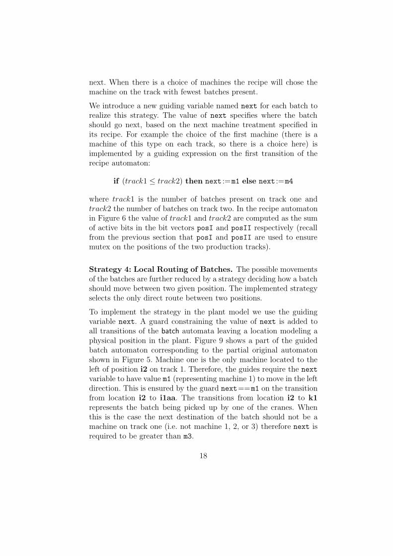
Strategy 4: Local Routing of Batches. The possible movementsof the batches are further reduced by a strategy deciding how a batchshould move between two given position. The implemented strategyselects the only direct route between two positions.

To implement the strategy in the plant model we use the guidingvariable next. A guard constraining the value of next is added toall transitions of the batch automata leaving a location modeling aphysical position in the plant. Figure 9 shows a part of the guidedbatch automaton corresponding to the partial original automatonshown in Figure 5. Machine one is the only machine located to theleft of position i2 on track 1. Therefore, the guides require the next

variable to have value m1 (representing machine 1) to move in the leftdirection. This is ensured by the guard next==m1 on the transitionfrom location i2 to i1aa. The transitions from location i2 to k1represents the batch being picked up by one of the cranes. Whenthis is the case the next destination of the batch should not be amachine on track one (i.e. not machine 1, 2, or 3) therefore next isrequired to be greater than m3.

18

Strategy 5: Moving of Cranes. When a crane is carrying a batchit always follows the strategy of the batch. If a crane is empty, thestrategy is to move only when something is ready to be picked up orif it is blocking the other crane. To allow a crane to move when it isblocking the other crane we enable the two cranes to communicate.

Guiding guards in the crane automata testing bits in posI and posII

ensure that the cranes move towards the pick up positions on thetracks only when a batch is waiting to be picked up (see e.g. thetransition from location c2emp to c2c1emp in Figure 14 of theAppendix). To allow an empty crane to move in other situations theguiding variables creq1 and creq2 are introduced. Guards testingtheir value are introduced on some transitions to allow the crane tomove from certain positions in a specified directions when the vari-ables are non-zero. The variables are typically assigned by the othercrane to indicate that it is moving towards a (possibly) occupiedposition that must be empty. For example, in the craneB automatonshown in Figure 14 the variable creq1 is assigned on the transitionsfrom location c2emp to c1emp to allow crane 1 to leave crane posi-tion 1 (modeled by the locations c1emp, c1up, c1down, and c1fullin the craneB automaton).

Other Strategies. It is possible to imagine other strategies andother experiments that would be interesting. However, the strategiespresented here have been very effective as shown by the results in thenext section. Using the approach to guiding presented here allows foreasy adding and changing of guides. This is important since guidesare based on heuristics so experimenting is sometimes needed forfinding good strategies.

5 Experimental Results

The plant models described in the previous sections have been ana-lyzed in the validation and verification tool Uppaal [LPY95,LPY97].In this section we present the results of the analysis for three versionsof the model, with varying number of guides and batches. In partic-ular, we present the measured time and space needed by Uppaal to

19

perform the analysis. Comparing the requirements for the differentmodels allows us to evaluate the benefits of the presented guidingtechniques. To evaluate the effect of adding guides, we use the stan-dard UNIX programs time and top to measure the CPU time andthe memory consumed by Uppaal when generating a trace from thetwo models.

The three analyzed models are: the original plant model without theguides described in Section 3, the plant model with all guides addeddescribed in Section 4, and a model with all guides added except theonce using the nextbatch variable described in Section 4.

Uppaal offers a number of options to control the internal verifi-cation algorithm applied in the tool [LPY97]. When analyzing theplant models we have used the compact data-structure for con-straints [LLPY97], the control-structure reduction [LLPY97], and arecently implemented version of the (in-)active clock reduction [DT98].In addition we experiment with using breadth-first (BFS), depth-firstsearch strategy (DFS), or depth-first search in combination with bit-state hashing (BSH) [Hol91]6.

All Guides Some Guides No Guides# BFS DFS BSH BFS DFS BSH BFS DFS BSH

sec MB sec MB sec MB sec MB sec MB sec MB sec MB sec MB sec MB

1 0.1 0.9 0.1 0.9 0.1 0.9 0.1 0.9 0.1 0.9 0.1 0.9 3.2 6.1 0.8 2.2 3.9 3.32 18.4 36.4 0.1 1.0 0.1 1.1 - - 2.1 4.4 7.8 1.2 - - 19.5 36.1 - -3 - - 3.2 6.5 3.4 1.4 - - 72.4 92.1 901 3.4 - - - - - -4 - - 4.0 8.2 4.6 1.8 - - - - - - - - - - - -5 - - 5.0 10.2 5.5 2.2 - - - - - - - - - - - -10 - - 13.3 25.3 16.1 9.3 - - - - - - - - - - - -15 - - 31.6 51.2 48.1 22.2 - - - - - - - - - - - -20 - - 61.8 89.6 332 46.1 - - - - - - - - - - - -25 - - 104 144 87.2 83.3 - - - - - - - - - - - -30 - - 166 216 124.2 136 - - - - - - - - - - - -35 - - 209 250 - - - - - - - - - - - - - -

Table 1. Time and space requirements for generating schedules.

6 The bit-state hashing technique generates a sub set of the reachable state-space. Afeasible schedule found with this technique is therefore guaranteed to also be feasiblein the original plant model.

20

Table 1 shows the time (in seconds) and space (in MB) consumedby Uppaal version 3.0.12 7 when generating schedules from thethree models. The numbers in the leftmost column corresponds tothe number of batches in the model (and in the generated schedule).We use the marker “-” to indicate that the corresponding executionrequires more than 256MB of memory, more than two hours of ex-ecution time, or that a suitable hash table size has not been found.When applying the hash table technique, we have used table sizesfrom 1048577 to 33554441 bits. The reported results corresponds tothe most suitable hash table sizes found.

As can be seen in Table 1, the use of guides significantly increases thesize of models that can be analyzed. In the guided model, schedulescan be generated for 35 batches using 250 MB in 3.5 minutes, whereasno schedule can be generated for three batches (or more) when noguides are used. We also observe that adding some guides improvesthe situation by enabling analysis of systems with three batches.

It can also be observed that the bit-state hashing technique does notallow analysis of larger models in this experiment, even though itperforms well space-wise on most models. We experienced that find-ing suitable hash table sizes is very tedious for large system models.The largest system analyzed in the experiment is therefore a guidedmodel using depth-first search strategy but without the bit-statehashing technique.

We have also installed Uppaal on a Sun Ultra machine equippedwith 1024MB of memory. On this machine, a schedule for 60 batchescan be generated from the guided model in 2 257 seconds.

6 Synthesis of Control Programs

We did not expect to be able to run the generated control programsin the original plant of SIDMAR. Therefore we have used a LEGOplant (see Figure 10) to run the synthesized programs in. This allowsfor experimenting with the plant to validate the model and it also

7 The tool was installed on a Linux Redhat 5.2 machine equipped with a Pentium IIIprocessor and 256MB of memory.

21

Fig. 10. The LEGO plant.

makes it easy to find answers to a number of questions about theplant (e.g. measuring time bounds).

The plant consists of a number of distributed units, each controlledlocally by one RCX [LEG98] brick. There are three types of unitsused in the plant: a crane, a machine with a track segment, andthe casting machine. For the cranes there is an overhead track. Theinterface to the units consists of a set of commands like MoveTrack-Right, TurnOnMachine, and LiftBatch. Commands are send to thelocal units by one central controller which is running the synthesizedprogram. Ideally, one would want the local controllers to give feed-back to the central controller when actions have finished or when anerror occurs. However, since the communication between the RCXbricks is slow and unreliable especially if more than one brick triesto send at one time, the only feedback from the local controllers areacknowledgements of commands received from the global controller.This has big influences on how the generated programs. There areno loops or branches in the control of the plant, only to implementcommunication between the RCX bricks are loops and branchesused.

22

As a result of the model checking in Uppaal a trace containing in-formation about synchronizations between automata and delays isobtained. Some of the synchronizations in the model, like the recipesynchronizing with the test automaton, are not relevant for the gen-erated schedule. To get a schedule for the plant we project the traceto the actions relevant for the plant. Given some numbering of tracksand machines, part of a schedule looks like in Figure 11. There is aone-to-one correspondence between a schedule of this kind and thecommands of the synthesized central control program. Each line witha Delay action is translated into a delay in the control program (inRCX code there is a Wait instruction doing this). For the rest ofthe lines only the second part is used, which defines what unit thecommand should be send to and what the command is. For examplein the line Load1.Track2Right, the part Track2Right is translatedto a command MoveTrackRight and sent to the local controller oftrack two.

... Delay(5)

Load1.Track1Right Crane1.Move1Left

Delay(10) Delay(5)

Load1.Machine1On Load1.Machine2On

Load2.Track5Right Delay(1)

Delay(4) Crane1.Move1Left

Crane1.Move1Left Delay(6)

Delay(6) Crane1.Move1Left

Load1.Machine1Off Delay(3)

Load1.Track2Right Load1.Machine2Off

Crane1.Pickup1 ...

Fig. 11. Part of a generated schedule.

The projection and the translation have been implemented using thepattern scanning and processing language gawk. Since the RCXlanguage does not offer reliable communication primitives, each linein the schedule is translated into a code segment implementing suchcommunication. Figure 12 shows a part of a synthesized control pro-gram. The language does not support functions or procedures there-fore the code implementing the communication has to be in-lined foreach instruction send to a local unit.

23

’’’’moveAup();

’’’’Crane A - Move UP

PB.PlaySystemSound 1

PB.SendPBMessage 2, 99 ’ Move up, on C1

PB.SetVar 1, 15, 0 ’Wait for ack

PB.While 0, 1, 3, 2, 99

PB.Wait 2, 20

PB.SetVar 1, 15, 0 ’Read the message

PB.ClearPBMessage

PB.SumVar 2, 2, 1

PB.If 0, 2, 2, 2, 20 ’If looped 20 times

PB.PlaySystemSound 1

PB.SendPBMessage 2, 99 ’Then Send message,

again same as sendig 0

PB.SetVar 2, 2, 0

PB.EndIf

PB.EndWhile

’’’’Delay 12

PB.Wait 2, 1200

Fig. 12. Part of a synthesized program.

The synthesized programs have been executed in the plant. This wasmainly intended as validation of the Uppaal model of the plant.During the validation we found three errors in the model: the cranestarted to move horizontally too early when an empty ladle waspicked up from the casting machine, causing the crane to collidewith the casting machine and accidently drop the lifted ladle, sohere a delay was missing in the model; when two cranes were locatedat positions next to each other and started to move in the samedirection they could collide because the crane ’in front’ was startedlast; in systems with only one batch the casting machine did notturn correctly. These problems were corrected in the model and newcontrol programs were synthesized.

At one point during the experiments with the plant the batteriesrunning the crane started to wear out. This meant that the initialtiming information obtained from the plant was inaccurate becausethe cranes were moving slower. At this point having the completeprocess from generating traces to synthesizing control programs fullyautomated proved especially useful. New times for the moving ofthe cranes were measured and put into the model. Since scheduling

24

still was possible, new programs were quickly synthesized and wererunning in the plant as expected.

Performing the experiments also validate the implementation of thetranslation from schedules to programs and here no problems werefound. Our confidence in the correctness of the model has been sig-nificantly increased by conducting these experiments.

7 Conclusion

In this paper, we have used timed automata and the verification toolUppaal to synthesize control programs for a batch production plant.To deal with the unavoidable complexity of a plant model suitablyaccurate for program synthesis, we suggest and apply a general ap-proach of guiding a model according to certain strategies. With thistechnique, we have been able to synthesize schedules for as many as60 batches on a machine with 1024 MB of memory. Applying bit-state hashing the space consumption may be decreased even further.

Based on traces from the model checking tool Uppaal, schedules aregenerated. From theses schedules, control programs are synthesizedand later executed in a physical plant. During execution a few mod-eling errors were detected. After correcting the model, new scheduleswere generated and correct programs were synthesized and executedin the plant.

The presented method for guiding model-checking has proved verysuccessful in significantly increasing the size of models which canbe analyzed. The largest model we analyze consists of 125 timed au-tomata and a total of 183 clocks. The notion of guides allows the userto add heuristics for controlling the behavior of the plant, and webelieve that the approach is applicable and useful for model check-ing in general and reachability checking in particular. The validationof the model by running the synthesized programs also proved use-ful: having access to the (a) physical plant during the design of themodel, allowed a number of questions to be readily answered.

Based on the traces generated from the Uppaal model other types ofcontrol programs can be synthesized. Here it would be especially in-teresting to study how more communication between the distributed

25

controllers can be used, e.g. for generating more optimal programs,and for detecting run-time errors. The guides added here decreasethe size of the state-space. However, most of the strategies presentedhere could also be realized by changing the search order to first searchthe states which are most likely to lead to a goal state. This wouldnot delete possible solutions, which would be particular useful if onewere searching for optimal schedules. Searching for optimal sched-ules, a notion of cost should be added to the model. Here an obviouschoice would be the time passed.

Acknowledgements: The authors wish to thank Ansgar Fehnkerand Kare Jelling Kristoffersen for fruitful discussions and many use-ful suggestions.

References

[AD94] R. Alur and D. Dill. Automata for Modelling Real-Time Systems. Theo-retical Computer Science, 126(2):183–236, April 1994.

[AL91] Martin Abadi and Leslie Lamport. The existence of refinement mappings.Theoretical Computer Science, 82:253–284, 1991.

[BGK+96] Johan Bengtsson, W.O. David Griffioen, Kare J. Kristoffersen, Kim G.Larsen, Fredrik Larsson, Paul Pettersson, and Wang Yi. Verification ofan Audio Protocol with Bus Collision Using Uppaal. In Rajeev Alur andThomas A. Henzinger, editors, Proc. of the 8th Int. Conf. on ComputerAided Verification, number 1102 in Lecture Notes in Computer Science,pages 244–256. Springer–Verlag, July 1996.

[BJLY98] Johan Bengtsson, Bengt Jonsson, Johan Lilius, and Wang Yi. Partial OrderReductions for Timed Systems. In Proc. of CONCUR ’98: ConcurrencyTheory, 1998.

[BS99] Rene Boel and Geert Stremersch. VHS Case Study 5: Timed Petri net modelof steel plant at SIDMAR. Technical report, SYSTeMS Group, UniversiteitGent, Technologiepark-Zwijnaarde 9, B-9052 Ghent, Belgium, 1999.

[DT98] Conrado Daws and Stavros Tripakis. Model checking of real-time reach-ability properties using abstractions. In Bernard Steffen, editor, Proc. ofthe 4th Workshop on Tools and Algorithms for the Construction and Anal-ysis of Systems, number 1384 in Lecture Notes in Computer Science, pages313–329. Springer–Verlag, 1998.

[Feh99] Ansgar Fehnker. Scheduling a steel plant with timed automata. In Pro-ceedings of the 6th International Conference on Real-Time Computing Sys-tems and Applications (RTCSA99), pages 280–286. IEEE Computer Soci-ety, 1999.

[Hol91] Gerard Holzmann. The Design and Validation of Computer Protocols. Pren-tice Hall, 1991.

26

[KLPW99] K. Kristoffersen, K. Larsen, P. Pettersson, and C. Weise. VHS Case Study 1- Experimental Batch Plant using UPPAAL. BRICS, University of Aalborg,Denmark, May 1999.

[LEG98] LEGO. Software developers kit, November 1998. Seehttp://www.legomindstorms.com/.

[LLPY97] Fredrik Larsson, Kim G. Larsen, Paul Pettersson, and Wang Yi. EfficientVerification of Real-Time Systems: Compact Data Structures and State-Space Reduction. In Proc. of the 18th IEEE Real-Time Systems Sympo-sium, pages 14–24. IEEE Computer Society Press, December 1997.

[LPY95] Kim G. Larsen, Paul Pettersson, and Wang Yi. Compositional and Sym-bolic Model-Checking of Real-Time Systems. In Proc. of the 16th IEEEReal-Time Systems Symposium, pages 76–87. IEEE Computer SocietyPress, December 1995.

[LPY97] Kim G. Larsen, Paul Pettersson, and Wang Yi. Uppaal in a Nutshell.Int. Journal on Software Tools for Technology Transfer, 1(1–2):134–152,October 1997.

[Mil89] R. Milner. Communication and Concurrency. Prentice Hall, EnglewoodCliffs, 1989.

[Sto00] M. Stobbe. Results on scheduling the sidmar steel plant using constraintprogramming. Internal report, 2000.

[YPD94] Wang Yi, Paul Pettersson, and Mats Daniels. Automatic Verificationof Real-Time Communicating Systems By Constraint-Solving. In DieterHogrefe and Stefan Leue, editors, Proc. of the 7th Int. Conf. on FormalDescription Techniques, pages 223–238. North–Holland, 1994.

Appendix

emptyempty

fullemptyx<=casttotal

fullempty2x<=casttotal

emptyfull

fullfullx<=casttotal

turningx<=castturn

fullfull2x<=casttotal

turning2

go finish?

x==casttotal

x:=0nrut!

x==casttotal

x:=0nrut!

outcast?

incast?

incast?

x==castturnturn!

x>=castturnoutcast?

x:=0turn!

caststart?

Fig. 13. The casting machine.

27

c1emp c1full

c2emp

c2c1emptCB<=cdelay

c2c1fulltCB<=cdelay

c2full

c3emp

c3c2emp

tCB<=cdelay

c3c2fulltCB<=cdelay

c3full

c4emp

c4c3emptCB<=cdelay

c4c3fulltCB<=cdelay

c4full

c5emp

c5c4emptCB<=cdelay

c5c4fulltCB<=cdelay

c5full

c2c1aemptCB<=cdelay

c3c2aemp

tCB<=cdelay

c4c3aemp

tCB<=cdelay

c5c4aemptCB<=cdelay

c2c1afulltCB<=cdelay




c2uptCB<=cup

c2downtCB<=cup

c1up tCB<=cup

c1downtCB<=cup

c3uptCB<=cup

c3downtCB<=cup

c4up

tCB<=cup

c4downtCB<=cup

c5uptCB<=cup

c5downtCB<=cup

cpos[3]==0, cpos[2]==0,posI[4]==1

cpos[3]:=1,cpos[4]:=0,tCB:=0,creq1:=1

moveBup?

tCB==cdelay,cpos[2]==0




evom21?

cpos[3]==0


moveB21?

cpos[5]==0


moveBup?


cpos[4]:=1,cpos[5]:=0


cpos[4]:=1,cpos[5]:=0

evom32?

cpos[5]==0

cpos[5]:=1,cpos[6]:=0,tCB:=0

move32?

cpos[7]+creq2==0

cpos[7]:=1,cpos[8]:=0,tCB:=0

moveBup?


cpos[6]:=1,cpos[7]:=0


cpos[6]:=1,cpos[7]:=0

evom43?

cpos[7]==0

cpos[7]:=1,cpos[8]:=0,tCB:=0

move43?

cpos[9]==0

cpos[9]:=1,cpos[10]:=0,tCB:=0

moveBup?


cpos[8]:=1,cpos[9]:=0


cpos[8]:=1,cpos[9]:=0

evom54?

cpos[9]==0

cpos[9]:=1,cpos[10]:=0,tCB:=0

move54?

cpos[3]==0,cpos[4]==0,posII[4]==1

cpos[3]:=1,cpos[2]:=0,tCB:=0

moveBdown?


cpos[4]:=1,cpos[3]:=0

cpos[5]==0,creq2==1

cpos[5]:=1,cpos[4]:=0,tCB:=0

moveBdown?


cpos[6]:=1,cpos[5]:=0

cpos[7]==0,creq2==2

cpos[7]:=1,cpos[6]:=0,tCB:=0

moveBdown?


cpos[8]:=1,cpos[7]:=0

cpos[9]==0,creq2==2

cpos[9]:=1,cpos[8]:=0,tCB:=0

moveBdown?


cpos[10]:=1,cpos[9]:=0

cpos[3]==0

cpos[3]:=1,cpos[2]:=0,tCB:=0

moveB12?


cpos[4]:=1,cpos[3]:=0

evom12?

cpos[5]==0

cpos[5]:=1,cpos[4]:=0,tCB:=0

move23?


cpos[6]:=1,cpos[5]:=0

evom23?

cpos[7]==0

cpos[7]:=1,cpos[6]:=0,tCB:=0

move34?


cpos[8]:=1,cpos[7]:=0

evom34?

cpos[9]==0

cpos[9]:=1,cpos[8]:=0,tCB:=0

move45?


cpos[10]:=1,cpos[9]:=0

evom45?

tCB:=0cBIIup?

tCB==cupposII[4]:=0

posII[4]==0tCB:=0, posII[4]:=1

cBIIdown_start?tCB==cup

cIIdown_end!

tCB:=0cBIup?

tCB==cupposI[4]:=0

posI[4]==0tCB:=0, posI[4]:=1

cBIdown_start?tCB==cupcIdown_end!

tCB:=0cIIIup? tCB==cup

tCB==cupcIIIdown?

creq2!=2tCB:=0cIVup? tCB==cup

tCB:=0 cIVdown_start?tCB==cupcIVdown_end!

tCB:=0cVup?

tCB:=0 cVdown_start?tCB==cupcVdown_end!

Fig. 14. The lower crane.

28

finalt1 t2 t3 terminus

finish!quality1? quality2? quality1?

Fig. 15. A test automaton for producing three batches.

III2

waiting

V3cast

V5k5 V6 cast

i0 i0a

tRB1<=bmove

i1 i1a

tRB1<=bmove

i2 i2a

tRB1<=bmove

i3 i3a

tRB1<=bmove

i4 i4a

tRB1<=bmove

i5

ii0

ii0atRB1<=bmove

ii1

ii1atRB1<=bmove

ii2

ii2atRB1<=bmove

ii3

k0

k1

k1k0

k2

k2k1

k3

k3k2

k4

k4k3

k4sink

k5

k5V3bk5k4

machine1 machine2 machine3

machine4

machine5

p1

p2

sink

source

x1

i0aatRB1<=bmove i1aa

tRB1<=bmove i2aatRB1<=bmove

i3aatRB1<=bmove

i4aatRB1<=bmove

ii0aatRB1<=bmove

ii1aatRB1<=bmove

ii2aatRB1<=bmove

c2down

c1down

c4down

c5down

preii0

tRB1<=bmove

preI0tRB1<=bmove

park>0park:=park-1 cIIIup!

next:=emp doneB1!outcast! creq2:=0 cVup!

posI[1]==0

posI[1]:=1,posI[0]:=0,tRB1:=0

b1right?tRB1==bmove,posI[2]==0

posI[2]:=1,posI[1]:=0

posI[3]==0,next!=m1

posI[3]:=1,posI[2]:=0,tRB1:=0

m1right?

M1on?

tRB1==bmove,posI[4]==0posI[4]:=1,posI[3]:=0

posI[5]==0,next>m1,next<m4

posI[5]:=1,posI[4]:=0,tRB1:=0

b2right?

next>m3

cAIup!

tRB1==bmove next==m3

tRB1:=0m2right?

M2on?

tRB1==bmove next==m3

tRB1:=0b3right?

tRB1==bmove

M3on?

tRB1==bmove,posII[0]==0

posII[0]:=1,posII[1]:=0

posII[1]==0,next==NA

posII[1]:=1,posII[2]:=0,tRB1:=0

m4left?

M4on?



posII[3]==0,next==m4

posII[3]:=1,posII[4]:=0,tRB1:=0b5left?



posII[5]==0,next!=m5

posII[5]:=1,posII[6]:=0,tRB1:=0m5left?

M5on?

move01!

next==NA move10!

next>m3

moveA12!

evom10!

evom01!

next<=m3

moveA21!

next==fin

move23!

next<=m3

evom21!

next>m3

evom12!

park<buf_size park:=park+1cIIIdown!

next==NAmove32!

next==fin

move34!

next==NA

evom32!

next==finevom23!

next==NAmove43!

dumpB1?

next==finmove45!

next==NAevom43!

next==finevom34!

next==emp

move54!

next!=emp

incast!

tryB1!

next==empevom54!

next==fin

evom45!

M1off? M2off? M3off?

M4off?

M5off?

next==m1,posI[0]==0

posI[0]:=1

goB1!

next==m4,posII[0]==0

posII[0]:=1

goB1!

next!=m4,next!=m5,next!=fin

cAIIup!

tRB1==bmove,posI[0]==0posI[0]:=1,posI[1]:=0

posI[1]==0,next==NA

posI[1]:=1,posI[2]:=0,tRB1:=0

m1left? tRB1==bmove,posI[2]==0posI[2]:=1,posI[3]:=0

posI[3]==0,next==m1

posI[3]:=1,posI[4]:=0,tRB1:=0

b2left?tRB1==bmove,posI[4]==0

posI[4]:=1,posI[5]:=0

next!=m2,next!=m3

tRB1:=0m2left?

tRB1==bmove

next!=m3

tRB1:=0b3left? tRB1==bmove

next!=m3

tRB1:=0m3left?

posII[1]==0


b4right?



posII[3]==0,next!=m4


m4right?



posII[5]==0,next==m5


b5right?



turn?

creq2:=2 nrut?

next>m3cAIIdown_start!

cIIdown_end?

next<=m3cAIdown_start!

cIdown_end?

cIVdown_start! cIVdown_end?

cVdown_start! cVdown_end?

next>m3,next!=fincBIIdown_start!

next!=m4,next!=m5

cBIIup!

next<=m3cBIdown_start!

next>m3

moveB12!

next<=m3

moveB21!

next>m3

cBIup!tRB1:=0b4right?

tRB1==bmove

tRB1:=0

b1right?

tRB1==bmove

Fig. 16. The batch automaton.

29

Recent BRICS Report Series Publications

RS-00-37 Thomas S. Hune, Kim G. Larsen, and Paul Pettersson.GuidedSynthesis of Control Programs for a Batch Plant usingUP-PAAL . December 2000. 29 pp. Appears in Hsiung, editor,International Workshop in Distributed Systems Validation andVerification. Held in conjunction with 20th IEEE InternationalConference on Distributed Computing Systems (ICDCS ’2000),DSVV ’00 Proceedings, 2000.

RS-00-36 Rasmus Pagh.Dispersing Hash Functions. December 2000.18 pp. Preliminary version appeared in Rolim, editor, 4th.International Workshop on Randomization and ApproximationTechniques in Computer Science, RANDOM ’00, Proceedingsin Informatics 8, 2000, pages 53–67.

RS-00-35 Olivier Danvy and Lasse R. Nielsen.CPS Transformation ofBeta-Redexes. December 2000. 12 pp.

RS-00-34 Olivier Danvy and Morten Rhiger.A Simple Take on Typed Ab-stract Syntax in Haskell-like Languages. December 2000. 25 pp.To appear in Fifth International Symposium on Functional andLogic Programming, FLOPS ’01 Proceedings, LNCS, 2001.

RS-00-33 Olivier Danvy and Lasse R. Nielsen.A Higher-Order ColonTranslation. December 2000. 17 pp. To appear inFifth In-ternational Symposium on Functional and Logic Programming,FLOPS ’01 Proceedings, LNCS, 2001.

RS-00-32 John C. Reynolds.The Meaning of Types — From Intrinsic toExtrinsic Semantics. December 2000. 35 pp.

RS-00-31 Bernd Grobauer and Julia L. Lawall. Partial Evaluation ofPattern Matching in Strings, revisited. November 2000. 48 pp.

RS-00-30 Ivan B. Damgard and Maciej Koprowski. Practical Thresh-old RSA Signatures Without a Trusted Dealer. November 2000.14 pp.

RS-00-29 Luigi Santocanale.The Alternation Hierarchy for the Theoryof µ-lattices. November 2000. 44 pp. Extended abstract ap-pears in Abstracts from the International Summer Conferencein Category Theory, CT2000, Como, Italy, July 16–22, 2000.

brics · brics rs-00-37 hune et al.: ... which is a case study of the vhs project1. ... to meet...

Documents