DH_rev_Dec12_2007

1

Basic NMR Concepts:

A Guide for the Modern Laboratory

Description:

This handout is designed to furnish you with a basic understanding of Nuclear Magnetic

Resonance (NMR) Spectroscopy. The concepts implicit and fundamental to the operation

of a modern NMR spectrometer, with generic illustrations where appropriate, will be

described. It can be read without having to be in front of the spectrometer itself. Some

basic understanding of NMR spectroscopy is assumed.

IMPORTANT: There is a short written test at the end of this handout, which must be

taken in order to obtain a NMR account.

This handout was prepared by Dr. Daniel Holmes of Michigan State University using the

NMR Basic Concepts handout from the University of Illinois’s NMR service facility,

under the direction of Dr. Vera V. Mainz. Her generous contribution is gratefully

acknowledged. February 2004.

Table of Contents:

Basic NMR Concepts.

I. Introduction 2

II. Basics of FT-NMR: Six critical parameters 3

III. Applications of FT-NMR 10

1) Shimming, line widths, and line shapes 12

2) Zero-filling 17

3) Apodization 20

4) Signal-to-noise measurements 22

5) Integration 25

6) Homonuclear decoupling 29

7) 13C-{1H} spectra 31

DH_rev_Dec12_2007

2

8) 13C-{1H} DEPT spectra 35

IV. Index 39

V. NMR Basics Test. 40

Introduction

Nuclear Magnetic Resonance (NMR) is a powerful non-selective analytical tool

that enables you to ascertain molecular structure including relative configuration, relative

and absolute concentrations, and even intermolecular interactions without the destruction

of the analyte. Once challenging and specialized NMR techniques have become routine.

NMR is indeed an indispensable tool for the modern scientist. Chemists, with little

knowledge of NMR, are now able to obtain 2- or even 3-dimensional spectra with a few

clicks of a button. Care must be taken, however, when using such ‘black box’

approaches. While the standard parameters used in the set-up macros for experiments

might be adequate for one sample, they may be wrong for another. A single incorrectly

set parameter can mean the difference between getting an accurate, realistic spectrum and

getting a meaningless result. A basic understanding of a few key aspects of NMR

spectroscopy can ensure that you obtain the best results possible. This guide is intended

to highlight the most pertinent aspects of practical NMR spectroscopy.

"Modern pulse NMR is performed exclusively in the Fourier Transform mode. Of

course it is useful to appreciate the advantages of the transform, and particularly the

spectacular results which can be achieved by applying it in more than one dimension, but

it is also essential to understand the limitations imposed by digital signal analysis. The

sampling of signals, and their manipulation by computer, often limit the accuracy of

various measurements of frequency and amplitude, and may even prevent the detection of

signals altogether in certain cases. These are not difficult matters to understand, but they

often seem rather abstract to newcomers to FT NMR. Even if you do not intend to operate

a spectrometer, it is irresponsible not to acquire some familiarity with the interaction

between parameters such as acquisition time and resolution, or repetition rate,

relaxation times and signal intensity. Many errors in the use of modern NMR arise

because of a lack of understanding of its limitations."

DH_rev_Dec12_2007

3

From A.E. Derome, Modem NMR Techniques for Chemistry Research (1987)

Basics of FT NMR- Six Critical Parameters

This section will give you enough information about FT-NMR experiments to

avoid the most common errors. We will cover the most important parameters that affect

any spectrum you may collect using an FT-NMR spectrometer. These are:

1. Spectrometer Frequency [sfrq]

2. Pulse Width [pw]

3. Acquisition Time [at]

4. Number of Points [np]

5. Sweep (Spectral) Width [sw]

6. Recycle Delay [d1]

[The letters in square brackets following the parameter represent the mnemonic used on

all Varian spectrometers. The parameters are discussed in more detail below.]

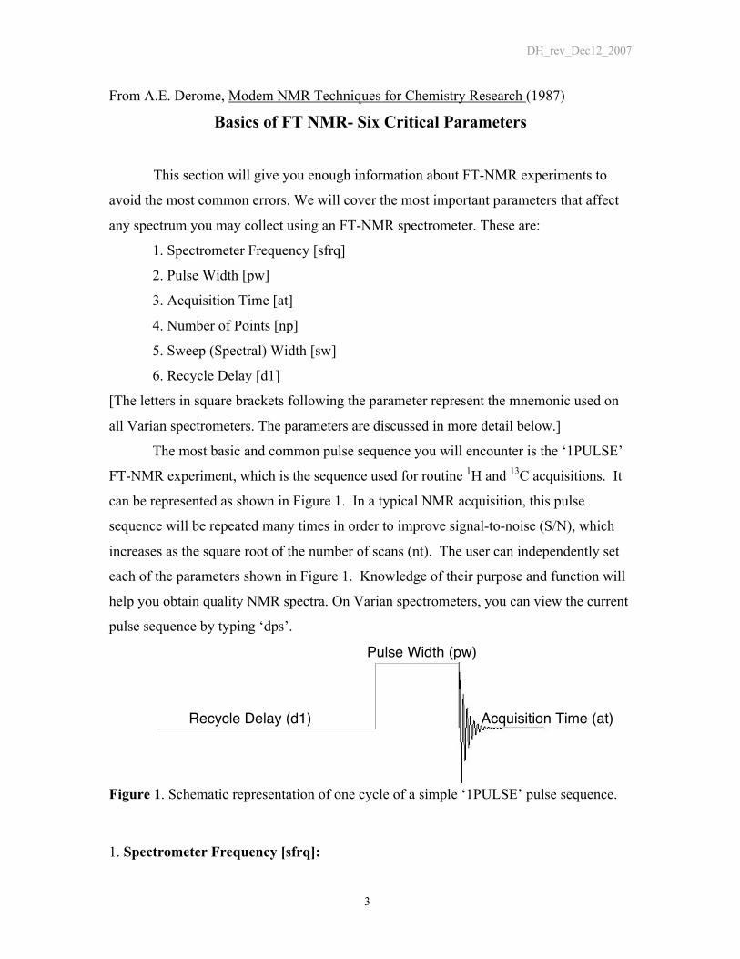
The most basic and common pulse sequence you will encounter is the ‘1PULSE’

FT-NMR experiment, which is the sequence used for routine 1H and 13C acquisitions. It

can be represented as shown in Figure 1. In a typical NMR acquisition, this pulse

sequence will be repeated many times in order to improve signal-to-noise (S/N), which

increases as the square root of the number of scans (nt). The user can independently set

each of the parameters shown in Figure 1. Knowledge of their purpose and function will

help you obtain quality NMR spectra. On Varian spectrometers, you can view the current

pulse sequence by typing ‘dps’.

Pulse Width (pw)

Recycle Delay (d1) Acquisition Time (at)

Figure 1. Schematic representation of one cycle of a simple ‘1PULSE’ pulse sequence.

1. Spectrometer Frequency [sfrq]:

DH_rev_Dec12_2007

4

It is called a “1PULSE” experiment because one radio frequency pulse (pw) is

applied per cycle. The radio frequency pulse excites the nuclei, which then re-radiate

during the acquisition time, giving an NMR signal in the form of an exponentially

decaying sine wave, termed free-induction decay (FID). The radio pulse has a

characteristic frequency, called the spectrometer frequency (sfrq), which is dependent

upon the nucleus you wish to observe and the magnetic field strength of the spectrometer.

NMR spectrometers are generally named for the frequency at which protons will

resonate. Thus, a Varian Inova 500 will cause protons to resonate at approximately 500

MHz. A 500 MHz NMR Spectrometer has a field strength of 11.7 Tesla. The

spectrometer frequency defines the center of the NMR spectrum you acquire.

A RF pulse with an exact frequency is not desirable since NMR chemical shifts

are spread out over a range of frequencies (~10 ppm for 1H and ~250 ppm for 13C).

Luckily, the short pulse lengths used in FT-NMR have a frequency spread due to the

Heisenberg Uncertainty Principle. As you shorten the pulse length and increase power,

uncertainty in the frequency results in a larger field of excitation. A longer, lower power

pulse will have less frequency spread and can be used for frequency selective excitation

or saturation.

2. Pulse width [pw]:

Prior to applying a radio pulse, a slight majority of nuclear spins are aligned

parallel to the static magnetic field (B0). The axis of alignment is typically designated the

Z-axis and the bulk magnetization is shown as a bold arrow (Figure 2, left side).

Application of a short radio frequency pulse at the appropriate frequency will rotate the

magnetization by a specific angle [θ=360(λ/2π)B1tp degrees, where (λ/2π)B1 is the RF

field strength and tp is the time of the pulse]. Pulses are generally described by this angle

of rotation (also called flip angle). The amount of rotation is dependent on the power

(tpwr) and width of the pulse in microseconds (pw). Maximum signal is obtained with a

90º pulse. Thus, a 90º pulse width is the amount of time the pulse of energy is applied to

the particular sample (90º is not 90º for all samples!) in order to flip all the spins into the

X-Y plane, i.e., the condition shown in Figure 2A. The 90º pulse width for proton NMR

experiments is set to about 8-13 µs on most instruments. The approximate field width of

excitation is given by the formula, RFfield =1/(4*90ºpulse). Thus, for a 8 µs, the field is

DH_rev_Dec12_2007

5

1/(4*0.000008) = 31250 Hz, which is ample for the typical range of proton resonances in

organic samples (at 500 MHz the proton range is about 5000 to 7000 Hz). The pulse

width is entered in microseconds by typing pw=desired value. The exact value is

dependent upon the sample (nucleus, solvent, etc.) as well as the instrument (probe, etc.).

Methods for measuring the pulse width will be discussed in another handout and are, for

the most part, only required for advanced experiments. For routine experiments, most

users use a 45º pulse for their data collection (Figure 2B). The reasons for this are

discussed under recycle delay.

Z

Y

XB0

PW= 10 µs (900)

Z

Y

X

900

A)

Y

XB0

X

Y

Z

PW= 5 µs (450)

Z

450

B)

Figure 2. The average nuclear spin magnetization (bold arrow) for an NMR sampleplaced in a magnetic field aligned along the Z-axis before and after application of a pulse.

3. Acquisition time (at):

Thus far, we have sent a pulse through the sample and flipped the magnetization

by a specific angle. The nuclear spins are no longer at equilibrium and will return to

equilibrium along the Z-axis. In Figure 1, the decaying sine wave represents this process

of Free Induction Decay (FID), which is a plot of emitted radio intensity as a function of

time. The time it takes to acquire the FID is called the acquisition time and is set by the

parameter ‘at’. A natural inclination might be to increase the acquisition time to

maximize the amount of signal that is acquired. Increasing the acquisition time is

advantageous up to a point, but will be detrimental if extended too far. Care and

DH_rev_Dec12_2007

6

forethought should be taken when adjusting ‘at’: too long and you will acquire noise

unnecessarily; too short and extraneous wiggles will occur at the base of the peaks (read

zero-filling section for more information).

4. Number of points (np):

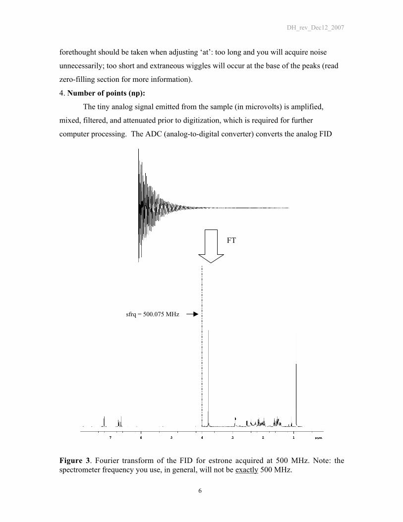
The tiny analog signal emitted from the sample (in microvolts) is amplified,

mixed, filtered, and attenuated prior to digitization, which is required for further

computer processing. The ADC (analog-to-digital converter) converts the analog FID

Figure 3. Fourier transform of the FID for estrone acquired at 500 MHz. Note: thespectrometer frequency you use, in general, will not be exactly 500 MHz.

FT

sfrq = 500.075 MHz

DH_rev_Dec12_2007

7

into a series of points along the FID curve. This is the number of points (np). In general,

the more points used to define the FID, the higher resolution. The number of points (np),

sweep width (sw), and acquisition time (at) are interrelated. Changing one of these

parameters will affect the other two (see below).

5. Sweep Width (sw):

While the FID contains all the requisite information we desire, it is in a form that

we cannot readily interpret. Fourier transforming the FID (commonly referred to as FT or

FFT for Fast Fourier Transform) will produce a spectrum with the familiar intensity as a

function of frequency, as shown in Figure 3. The frequency domain spectrum has two

important parameters associated with it: the spectrometer frequency (sfrq), discussed

earlier, and the spectral width or sweep width (referred to as sw- see Figure 4). It is

important to remember that the spectral width in ppm is independent of the spectrometer

operating frequency; however, since the number of Hz per ppm is dependent on the

spectrometer operating frequency, the spectral width in Hz will change depending upon

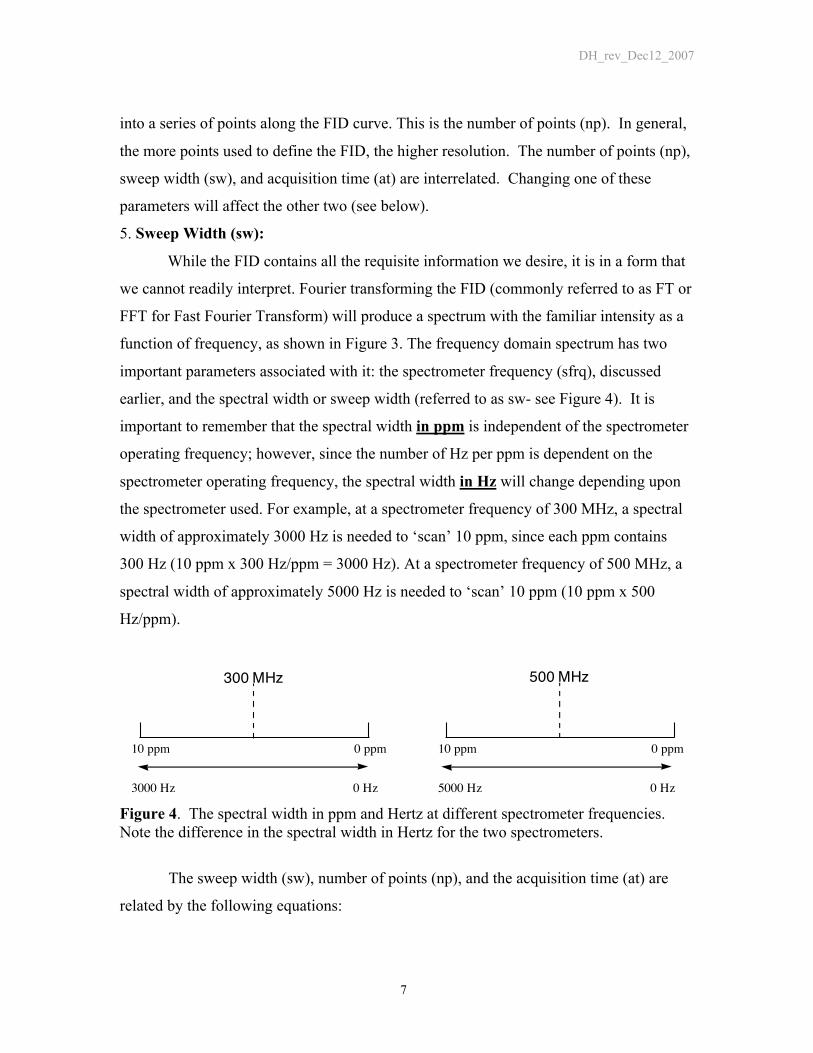
the spectrometer used. For example, at a spectrometer frequency of 300 MHz, a spectral

width of approximately 3000 Hz is needed to ‘scan’ 10 ppm, since each ppm contains

300 Hz (10 ppm x 300 Hz/ppm = 3000 Hz). At a spectrometer frequency of 500 MHz, a

spectral width of approximately 5000 Hz is needed to ‘scan’ 10 ppm (10 ppm x 500

Hz/ppm).

300 MHz 500 MHz

10 ppm 0 ppm 10 ppm 0 ppm

3000 Hz 0 Hz 5000 Hz 0 Hz

Figure 4. The spectral width in ppm and Hertz at different spectrometer frequencies.Note the difference in the spectral width in Hertz for the two spectrometers.

The sweep width (sw), number of points (np), and the acquisition time (at) are

related by the following equations:

DH_rev_Dec12_2007

8

€

at =np2sw

(1)

and

€

res =1at

=2swnp

(2)

where ‘res’ is the digital resolution of the spectrum. The digital resolution is in units of

Hz/point, and the rule-of-thumb is that the digital resolution (in Hertz) should be less than

one half the peak width at half-height. This ensures that each peak is described by at least

3 points. For example, if your peak width at half-height is 0.5 Hz, the digital resolution

should be less than 0.25 Hz. Therefore, if your spectrometer frequency is 500 MHz, your

total spectral width is 5000 Hz (10 ppm) and your required digital resolution (Res) is 0.25

Hz/point, rearranging equation 2 gives you the minimum number of points required for

adequate digital resolution:

€

np =2swres

= 40,000 points (3)

Since the computer works most efficiently if the number of points is a power of 2,

the closest larger power of 2 would automatically be used, which, in this case, is 65,536

points. The spectral width, number of points, and acquisition time can be specified when

operating the spectrometer, usually by typing the appropriate mnemonic followed by an

equals sign and the numeric value (e.g. np=64000). The spectrometer will set the units

automatically. Generally, Varian’s automatically change the number of points according

to equation 2 if the acquisition time or sweep width are changed. If at, np, or sw are

changed, the data must be reacquired. An alternative to changing these parameters is to

use ‘zero-filling’. This is described in the section titled ‘Zero-Filling’.

6. Recycle delay (d1):

On Varian’s this delay time is named d1 (pronounced dee-one) and appears at the

beginning of the pulse sequence (see Figure 1). In practice, this delay should be thought

DH_rev_Dec12_2007

9

of as coming after the acquisition time. It is an important parameter and plays a vital role

in obtaining accurate integration. After the RF pulse, the nuclear spins do not instantly

return to equilibrium; rather, they relax according to a time constant called T1 (T1 is 1/R,

where R is the rate of relaxation. After one T1, approximately 63% of the magnetization

has returned to the Z-axis). T1’s are dependent on many factors including nuclear

environment, temperature, and solvent. Carbon T1’s are typically much longer than

proton T1’s. Since each nucleus in a molecule is immersed in a different magnetic

environment, their T1’s will not be the same. Not allowing enough time for relaxation

between pulses will cause varied attenuation of the signals and inaccurate integration (see

Integration Section for more details). Normally, when a 90° pulse width is used to excite

the spins (Figure 2A), a total time (TT) between pulses of 5xT1 is necessary in order to

have complete relaxation. If a pulse width less than 90° is used, the total time can be

proportionally less. This is why the standard pulse width for 1D 1H NMR experiments is

45º.

The total time between scans is given by the following equation, where TT is the

total time and d1 is the recycle delay: TT = pw + at + d1.

Since the pulse width is in microseconds while the acquisition time and recycle

delay are in seconds, the pulse width can be ignored, leaving us with the equation:

€

TT = at + d1 (4)

The optimum recycle delay can be computed by rearranging the equation to give

€

d1= TT − at (5)

As an example of the above, if your longest T1 is 600 msec, then the total time (where

TT=5x T1) must be at least 3 seconds.

Take Home Lesson

These six parameters provide the foundation on which all NMR experiments are

built. Appreciation of them will go far in the correct acquisition and interpretation of

your NMR spectra, thus, saving precious time and effort. This not only applies to simple

DH_rev_Dec12_2007

10

1PULSE experiments, but also is equally important in 2-D and 3-D NMR spectroscopy.

DH_rev_Dec12_2007

11

Applications of FT-NMR1. CHCl3 Peak Width at Half Height (LW1/2).

The purpose of this section is to acquaint you with proper peak shape and the

problems that are caused by improper shimming.

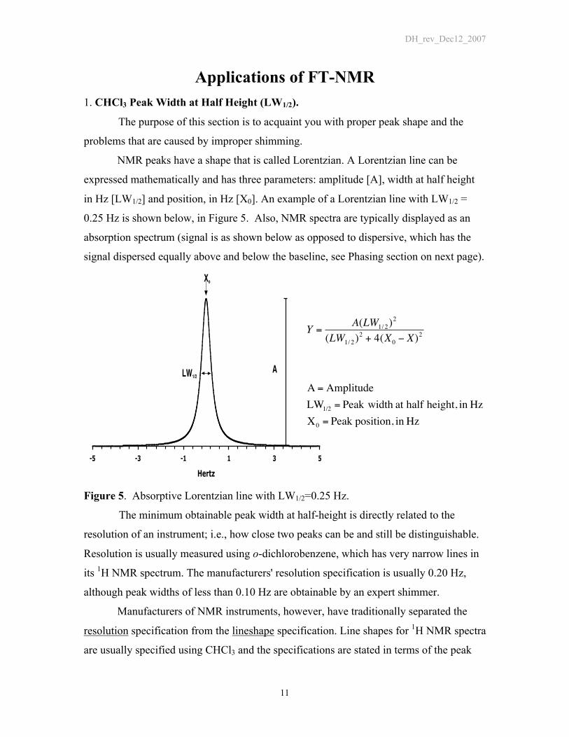
NMR peaks have a shape that is called Lorentzian. A Lorentzian line can be

expressed mathematically and has three parameters: amplitude [A], width at half height

in Hz [LW1/2] and position, in Hz [X0]. An example of a Lorentzian line with LW1/2 =

0.25 Hz is shown below, in Figure 5. Also, NMR spectra are typically displayed as an

absorption spectrum (signal is as shown below as opposed to dispersive, which has the

signal dispersed equally above and below the baseline, see Phasing section on next page).

-5 -3 -1 1 3 5

Hertz

LW1/2

Xo

A

Figure 5. Absorptive Lorentzian line with LW1/2=0.25 Hz.

The minimum obtainable peak width at half-height is directly related to the

resolution of an instrument; i.e., how close two peaks can be and still be distinguishable.

Resolution is usually measured using o-dichlorobenzene, which has very narrow lines in

its 1H NMR spectrum. The manufacturers' resolution specification is usually 0.20 Hz,

although peak widths of less than 0.10 Hz are obtainable by an expert shimmer.

Manufacturers of NMR instruments, however, have traditionally separated the

resolution specification from the lineshape specification. Line shapes for 1H NMR spectra

are usually specified using CHCl3 and the specifications are stated in terms of the peak

€

Y =A(LW1/ 2)

2

(LW1/ 2)2 + 4(X0 − X)

2

A = AmplitudeLW1/2 = Peak width at half height, in HzX0 = Peak position, in Hz

DH_rev_Dec12_2007

12

width at half-height, 0.55%, and 0.11 % height of the CHCl3 peak. The latter two

percentages are chosen because they are the height of the l3C satellites of the CHCl3 line

and one-fifth this height. These values are meaningful only when compared with the

half-height width. From the mathematical equation for a Lorentzian line (see Figure 5),

the line width at 0.55% height is calculated to be 13.5 times LW1/2, while the line width

at 0.11 % height is calculated to be 30 times the LW1/2. So, if the peak width at half-

height is 0.30 Hz, the calculated values are 4.0 Hz at 0.55% and 9.0 Hz at 0.11 %. For

comparison, the manufacturer's specifications are 10-15 Hz and 20-30 Hz at 0.55%

height and 0.11 % height, respectively. These values are larger than the theoretical values

because the line widths at 0.55% and 0.11 % height are very sensitive to shimming.

Other factors that influence line shape include the quality of the NMR tube, sample

spinning, sample concentration, dissolved oxygen, and paramagnetic impurities. The

latter three will lead to an overall broadening of the lines.

Phasing:

Due, in part, to delays in the pulse sequence between excitation and reception and

to frequency offset errors; acquired spectra will have a mix of absorptive and dispersive

signals. Your spectrum’s peaks will not look like the lorentzian in Figure 5, but have

some portion that is displaced below the baseline. As a user, you will have to correct the

spectrum by adjusting the ‘phase’ of the spectrum. The ‘Plotting Practice’ handout will

help you with phasing spectra. For now, it is only important to know that phasing the

spectrum is routine and involves correcting two parameters: zero-order phase, which is

frequency independent; and first-order phase, which is frequency dependent. Correcting

the phase is as simple as typing a command or doing a little bit of ‘click-and-drag’ mouse

work. Below is an example of a ‘poorly’ phased spectrum at left along with the correct

spectrum (i.e. purely absorptive peaks).

Not Phased Well Phased

DH_rev_Dec12_2007

13

Shimming:

The term ‘shimming a magnet’ is a piece of NMR jargon that harks back to the

early days of NMR spectroscopy. Originally, permanent magnets were used to provide

the external magnetic field. To obtain the most homogenous field across the sample, the

pole faces of the magnet had to be perfectly aligned, and to accomplish this, small pieces

of wood, or ‘shims’, were hammered into the magnet support, so as to physically move

the poles relative to each other. Luckily, nowadays you will not be required to bring

hammer and wooden shims to the spectrometer. Shimming is accomplished by changing

the applied current for a set of coils surrounding the probe. This applied current will

create small magnetic fields in the region of your sample that will either enhance or

oppose the static magnetic field. Your goal will be to adjust these coil fields by a series of

mouse clicks to obtain the most homogeneous magnetic field across your sample, which

is usually observed as an increase in the lock signal.

It is important for you to have a basic understanding of line shape so you can

judge when: (1) your shimming is off, and (2) you need to spend more time shimming

your sample. The best way to avoid problems is to establish a procedure, such as the one

detailed below.

I. Always load a shim library when you sit down at the instrument. You

should never assume the previous user left the instrument with a standard

shim library loaded. Without reloading standard shims, you will have to

start where the last person stopped - and that might include someone who

shimmed for a short sample, a bad tube, a viscous sample, etc.

II. Be aware of lock parameters, especially if you only shim on the lock

display. Establish lock transmitter power and gain levels that work for

most of your samples. If you encounter a sample that seems to require an

unusually high power or gain setting, there is a problem with your sample

and/or the instrument, and shimming on the lock level may be difficult or

impossible.

III. Shimming problems are confirmed only if the problem is visible on every

peak in your spectrum. If, for example, only one peak is doubled, the

problem is sample related, and can't be shimmed away. Remember,

DH_rev_Dec12_2007

14

anomalies close to the base of intense single lines may not be visible on

less intense peaks unless the vertical scale is increased.

IV. Establish a shimming method. Shimming is an ‘art form’ that requires

patience and practice. You should always approach shimming with some

method that works for you to give acceptable results. Example: load a

shim library; adjust the lock level to a maximum with Z1, then Z2, then

Z1, then Z3, and then Z1.

V. Spinning side bands should always be below 2%. If spinning side bands

are above 2%, turn off the spinner air, optimize the X and Y shims, then

turn the spinner air back on and re-optimize Z1, Z2, and Z3. If this does

not solve the problem, consider transferring your sample to another tube.

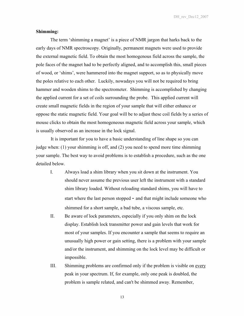
Knowledge of correct line shape can help you correct problems such as those

shown in Figure 6. Although the peak in Figure 6b may have a line width at half-height

that is less than 0.50 Hz, it is obviously poorly shimmed. You should never accept a

poorly shimmed line shape such as is shown in Figure 6b, where a single line is expected.

On the pages that follow are some line shape defects and the shims that should be

adjusted to correct the problem. You will also notice that the FID will show the problem

as well, but may not be as easy to diagnose. In general, odd-order shims (Zl, Z3, Z5)

affect the line shape symmetrically while even-order shims (Z2, Z4) cause a non-

symmetrical line shape. The higher the order (Z4 is higher order than Z2), the lower

(closer to the base of the peaks) the problem is observed.

DH_rev_Dec12_2007

15

DH_rev_Dec12_2007

16

Figure 6. From G. Chmurny and D. Hoult, “The ancient and honorable art of shimming.”Concepts in Magnetic Resonance, 1990, 2, 131-149.

Shimming Take Home Lesson

DH_rev_Dec12_2007

17

The ‘art’ of shimming resides in the fact that there is no single set of rules that

work for every sample, spectrometer, person, or even time of year. Personal experience

is the best and, frankly, only way to master shimming. That being said, knowledge of

correct line shapes will allow you to decide quickly whether your sample is correctly

shimmed. You will have to decide whether the return (a better line shape) is worth the

time spent achieving that line shape.

DH_rev_Dec12_2007

18

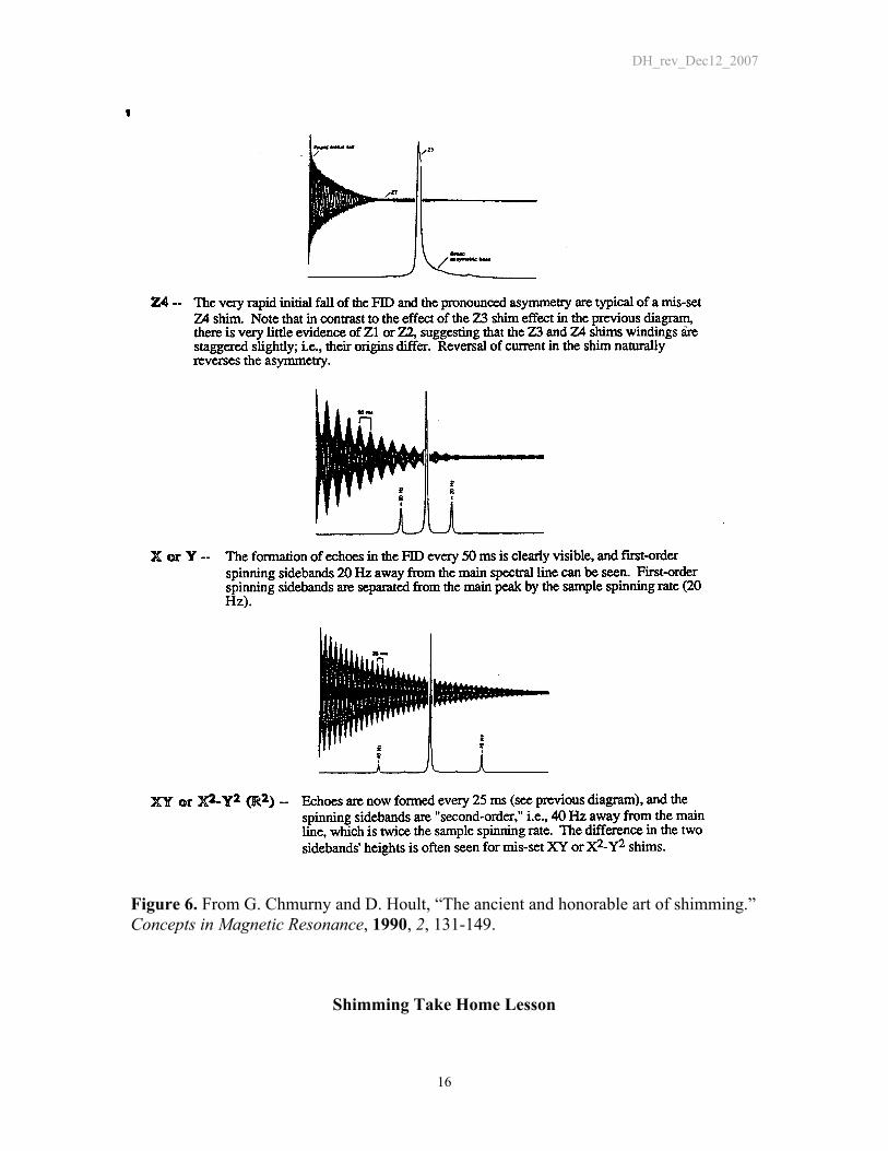
Zero-Filling

As stated earlier, the digital resolution is equal to (acquisition time)-1. If you

wanted to increase resolution, you might consider increasing the acquisition time (at) to

gain more points and, thus, better resolution. This would certainly work, but increasing it

too much would sacrifice Signal-to-Noise for the resolution enhancement. The FID has a

finite lifetime, which is proportional to the various T1’s for a given molecule. When the

acquisition time is significantly longer than the longest T1, the contribution from noise

will be quite large. This combined with the increased overall experimental time

Figure 7. Four scan acquisition of ethylbenzene on an Inova-300. The triplet to the rightwas acquired with at = 20 seconds, the triplet at left had at = 4 seconds, which gave a S/Ntwice that of the other acquisition. The FID’s are shown below the spectra.

DH_rev_Dec12_2007

19

necessary to acquire a given number of scans leads to a significant decrease of S/N.

Figure 7 shows the results from two separate acquisitions on the same sample with the

same number of scans, but with their acquisitions times differing by a factor of five. The

Signal-to-Noise for the 4-second acquisition time (at) is about twice that of the 20-second

acquisition time and required a fourth of the time. Note the FID’s, which clearly show

that the signal decays below the level of noise around two seconds. The additional

acquisition time merely adds noise to the spectrum.

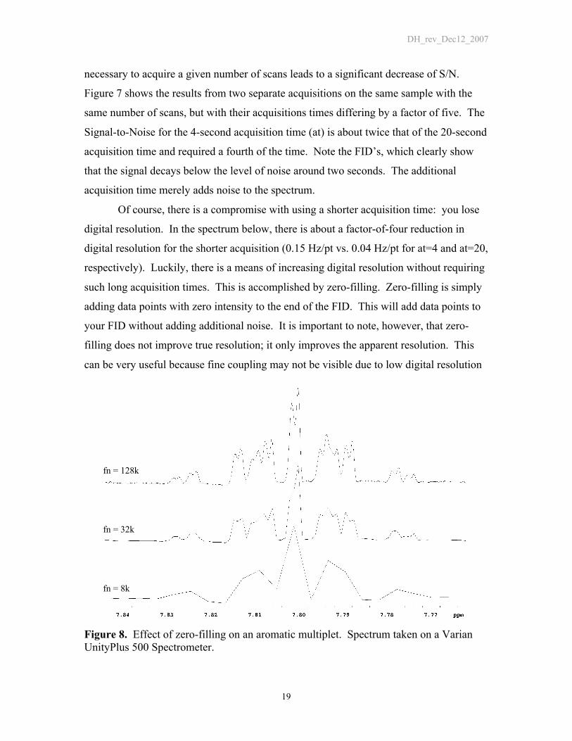
Of course, there is a compromise with using a shorter acquisition time: you lose

digital resolution. In the spectrum below, there is about a factor-of-four reduction in

digital resolution for the shorter acquisition (0.15 Hz/pt vs. 0.04 Hz/pt for at=4 and at=20,

respectively). Luckily, there is a means of increasing digital resolution without requiring

such long acquisition times. This is accomplished by zero-filling. Zero-filling is simply

adding data points with zero intensity to the end of the FID. This will add data points to

your FID without adding additional noise. It is important to note, however, that zero-

filling does not improve true resolution; it only improves the apparent resolution. This

can be very useful because fine coupling may not be visible due to low digital resolution

Figure 8. Effect of zero-filling on an aromatic multiplet. Spectrum taken on a VarianUnityPlus 500 Spectrometer.

fn = 128k

fn = 8k

fn = 32k

DH_rev_Dec12_2007

20

even though the coupling is resolved in the time domain. Figure 8 shows the effect of

zero-filling on a spectrum. At low resolution the fine coupling is not visible, but with

adding zeros to the FID, the details of coupling emerge. Varian executes zero-filling

through the Fourier number (fn). A Fourier transform will transform fn zeros to the

nearest power of two minus np points (e.g. if np=64k and fn=4*np, then the numbers of

zeros = 218 – 216 or 196608 points. A total of 262144 points will be transformed). In

practice, setting fn more than 4 times np is not useful.

One might be tempted by the preceding section to set the acquisition time (at) to a

very short value and then use zero-filling to increase the digital resolution. This will lead

to spectral artifacts. Figure 9 demonstrates these artifacts for the methyl triplet of ethyl

benzene. The spectrum on left has an acquisition time of 1 second and 4 seconds for the

one to the right. They both have the same number of points (200k), but clearly the

spectrum to the left has artifacts. These artifacts are termed truncation artifacts or,

colloquially, sinc wiggles [(sin x)/x modulation] and arise from turning off the receiver

before the FID has mostly decayed.

Figure 9. Truncation artifacts or so-called “sinc wiggles” because of too short acquisitiontime (at=1). Both spectra have 200k points. That to the right has an at=4 seconds withzero-filling to 200k. That to the left has at=1 seconds with zero-filling to 200k. Spectrawere taken on a Varian UnityInova 300.

DH_rev_Dec12_2007

21

Apodization

Signal-to-Noise (S/N) is very important for any spectroscopic technique. NMR

spectroscopy, unfortunately, suffers from low S/N. Acquiring more scans is the most

straightforward, if not time-consuming, means of improving S/N (S/N increases as the

square root to the number of scans. i.e. S/N ~√nt). An alternative approach is to apply a

weighting function to the FID to improve Signal-to-Noise. Also, you can apply

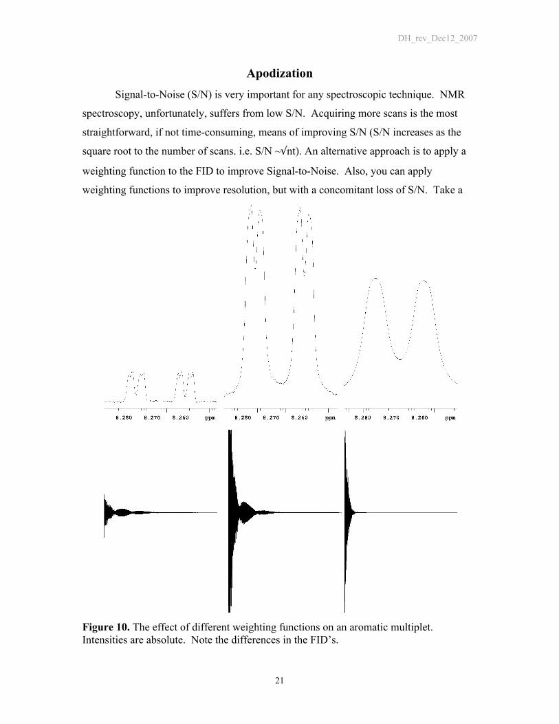
weighting functions to improve resolution, but with a concomitant loss of S/N. Take a

Figure 10. The effect of different weighting functions on an aromatic multiplet.Intensities are absolute. Note the differences in the FID’s.

DH_rev_Dec12_2007

22

look at Figure 10. The three sets of peaks and their corresponding FID’s are from the

same experiment. The only difference between the peaks is the particular type of

weighting function or apodization that was used. The set in the middle had no

apodization and we see an apparent doublet-of-doublets (J = 8.7 and 1.7 Hz). The S/N

for these peaks is 195.2 (the next section will describe the measurement of S/N.). Since

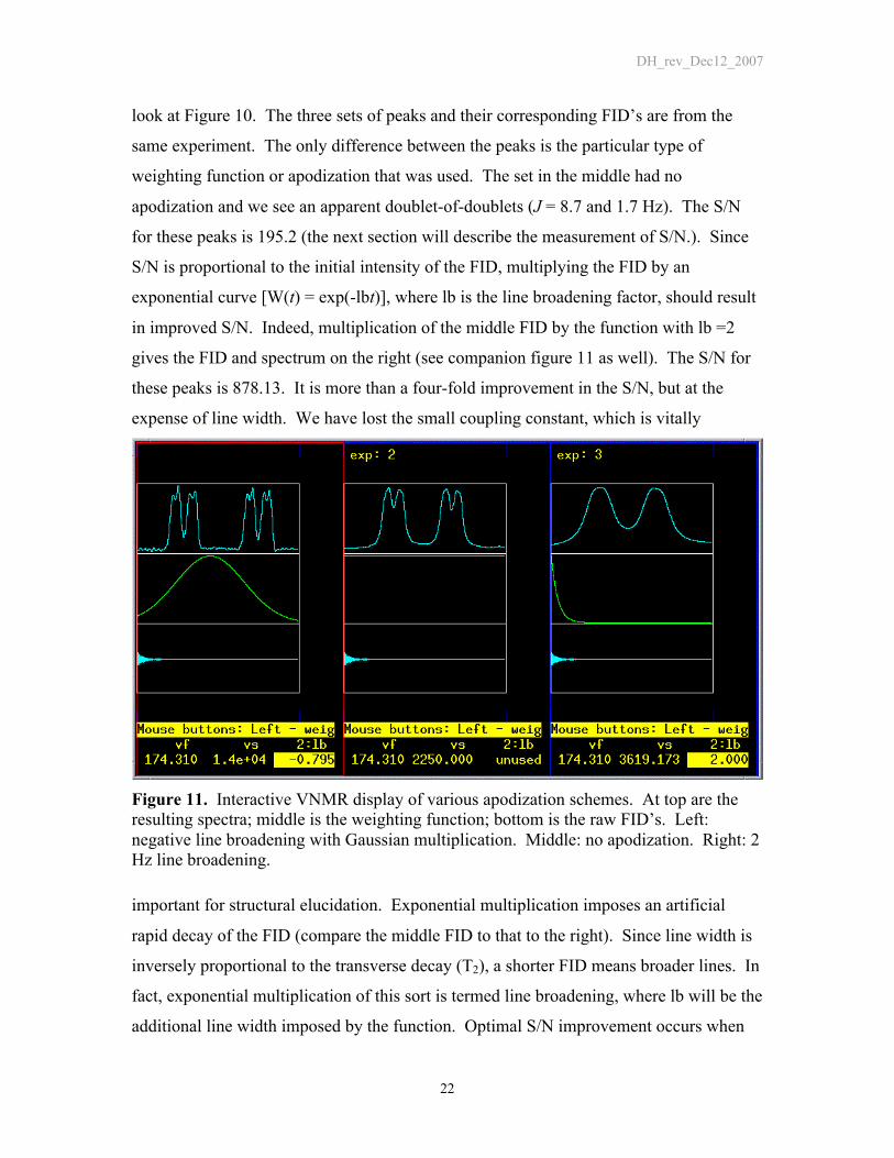
S/N is proportional to the initial intensity of the FID, multiplying the FID by an

exponential curve [W(t) = exp(-lbt)], where lb is the line broadening factor, should result

in improved S/N. Indeed, multiplication of the middle FID by the function with lb =2

gives the FID and spectrum on the right (see companion figure 11 as well). The S/N for

these peaks is 878.13. It is more than a four-fold improvement in the S/N, but at the

expense of line width. We have lost the small coupling constant, which is vitally

Figure 11. Interactive VNMR display of various apodization schemes. At top are theresulting spectra; middle is the weighting function; bottom is the raw FID’s. Left:negative line broadening with Gaussian multiplication. Middle: no apodization. Right: 2Hz line broadening.

important for structural elucidation. Exponential multiplication imposes an artificial

rapid decay of the FID (compare the middle FID to that to the right). Since line width is

inversely proportional to the transverse decay (T2), a shorter FID means broader lines. In

fact, exponential multiplication of this sort is termed line broadening, where lb will be the

additional line width imposed by the function. Optimal S/N improvement occurs when

DH_rev_Dec12_2007

23

the lb factor equals the resonances’ natural line width. Each resonance has its own line

width and, therefore, a single lb value will not be optimal for every peak.

Apodization can also be used to improve resolution by emphasizing the tail of the

FID. This has been done to the FID on the left of Figure 10. A function with a negative

line broadening factor as well as a Gaussian function has been used (see Figure 11, for

the VNMR interactive weighting window, which displays the function to the left). This

has emphasized the middle and end of the FID and has revealed an additional coupling of

0.6 Hz. In effect it has extended the length of the signal. The price to pay for this

apodization is a significant decrease in S/N; namely, from 195.2 to 60.8. Thus, you must

use such weighting schemes with caution. Furthermore, apodization cannot make up for

poor shimming or inadequate acquisition time. If it is not resolved in the time domain, it

will not be resolved using either zero-filling or apodization.

Signal-to-Noise Measurement

The signal-to-noise measurement, or S/N, is an important criterion for accurate

integrations, and is also one of the best ways to determine the sensitivity of a NMR

spectrometer. In general, a higher S/N specification means that the instrument is more

sensitive. It is also useful in roughly determining the time requirement for an experiment.

Standard S/N measurements for proton spectra are always determined using a

sample of 0.1 % ethylbenzene in CDCl3 (ETB). A typical result for the Varian Inova 500

is 200:1 using the 5mm probe. It is important that the spectrum be acquired under the

following standard conditions (only for determining system performance):

1. Use a 90 pulse.

2. Line Broadening of 1.0 Hz.

3. Spectral Width of 15 to 5 ppm.

4. A sufficient relaxation delay (at least 5xT1).

5. A sufficient digital resolution (less than 0.5 Hz/point).

6. One scan.

DH_rev_Dec12_2007

24

Optimum signal-to-noise for any sample is achieved using a line broadening

equal to the peak width at half height. When this line broadening is applied, the peak

width at half-height doubles, i.e., it is the sum of the natural peak width at one-half height

plus the line broadening applied. The equation used for calculating S/N is:

€

S /N =2.5ANpp

(5)

(where A = height of the chosen peak and Npp = peak-to-peak noise).

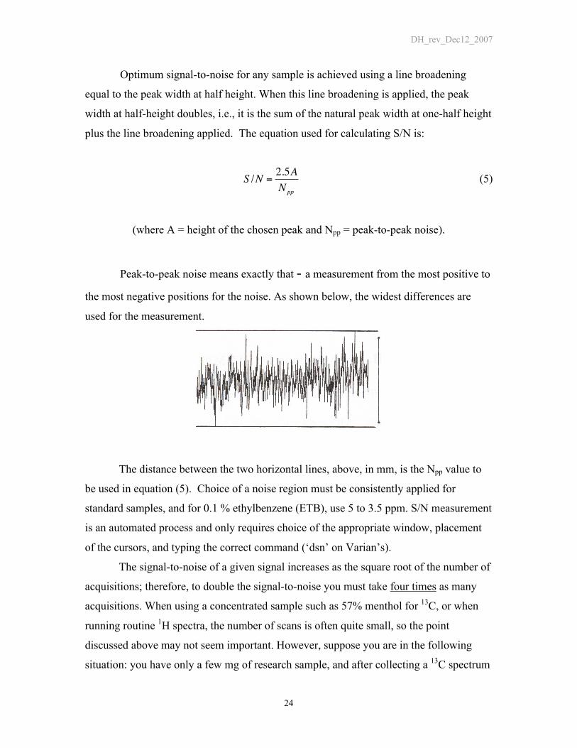
Peak-to-peak noise means exactly that - a measurement from the most positive to

the most negative positions for the noise. As shown below, the widest differences are

used for the measurement.

The distance between the two horizontal lines, above, in mm, is the Npp value to

be used in equation (5). Choice of a noise region must be consistently applied for

standard samples, and for 0.1 % ethylbenzene (ETB), use 5 to 3.5 ppm. S/N measurement

is an automated process and only requires choice of the appropriate window, placement

of the cursors, and typing the correct command (‘dsn’ on Varian’s).

The signal-to-noise of a given signal increases as the square root of the number of

acquisitions; therefore, to double the signal-to-noise you must take four times as many

acquisitions. When using a concentrated sample such as 57% menthol for 13C, or when

running routine 1H spectra, the number of scans is often quite small, so the point

discussed above may not seem important. However, suppose you are in the following

situation: you have only a few mg of research sample, and after collecting a 13C spectrum

DH_rev_Dec12_2007

25

for 2 hours, you get peaks with an S/N of only 5:1. Since the peaks are barely visible

above the noise (and you may have missed any quaternary carbons), you want to re-

collect the spectrum to get an S/N of 50:1, a value more typical for carbon NMR.

Unfortunately, this will take 10 * l0 * 2 = 200 hours!

S/N Take Home Lesson

At some point, you may take a spectrum and wonder why the signals are so weak.

Over 75% of the time, the problem is not with the spectrometer, but with your sample.

You can test this quickly by taking a spectrum of a standard such as ETB or menthol. In

this way, you can save yourself needless frustration by identifying problems that are due

to a bad sample. Always obtain the spectrum of a standard, well-characterized compound

before obtaining that of your unknown.

DH_rev_Dec12_2007

26

Integration

The purpose of this section of the handout is to show you how to obtain accurate

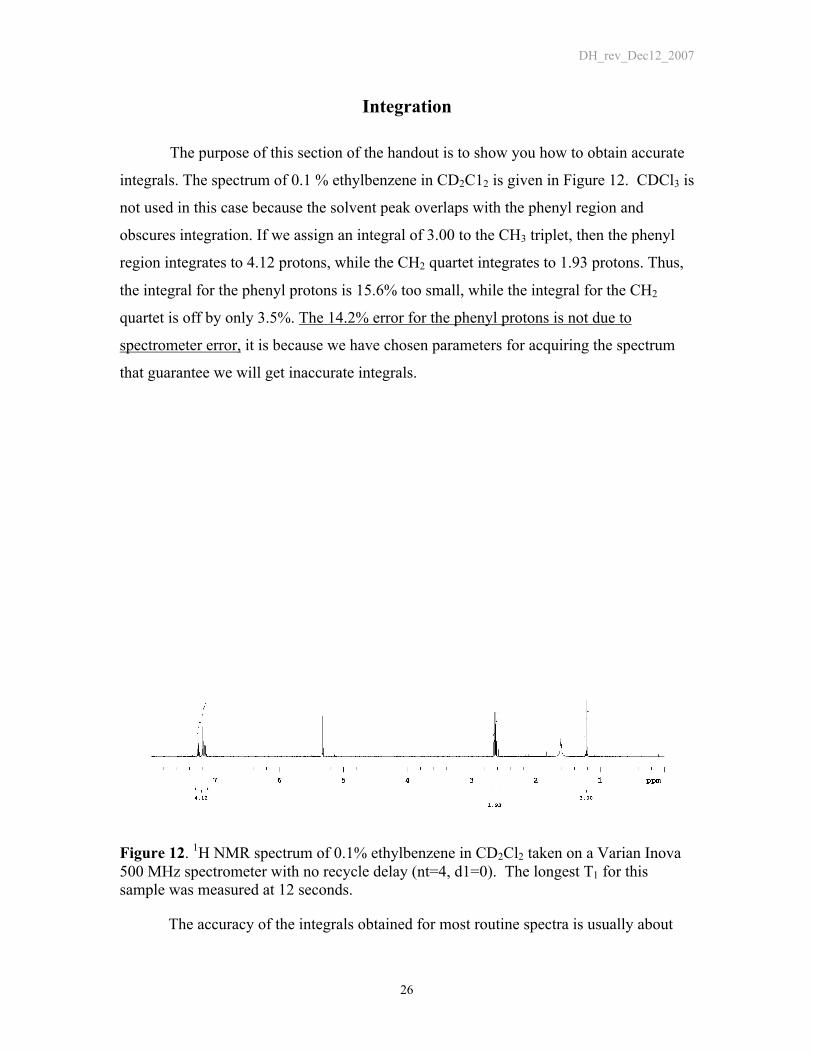
integrals. The spectrum of 0.1 % ethylbenzene in CD2C12 is given in Figure 12. CDCl3 is

not used in this case because the solvent peak overlaps with the phenyl region and

obscures integration. If we assign an integral of 3.00 to the CH3 triplet, then the phenyl

region integrates to 4.12 protons, while the CH2 quartet integrates to 1.93 protons. Thus,

the integral for the phenyl protons is 15.6% too small, while the integral for the CH2

quartet is off by only 3.5%. The 14.2% error for the phenyl protons is not due to

spectrometer error, it is because we have chosen parameters for acquiring the spectrum

that guarantee we will get inaccurate integrals.

Figure 12. 1H NMR spectrum of 0.1% ethylbenzene in CD2Cl2 taken on a Varian Inova500 MHz spectrometer with no recycle delay (nt=4, d1=0). The longest T1 for thissample was measured at 12 seconds.

The accuracy of the integrals obtained for most routine spectra is usually about

DH_rev_Dec12_2007

27

10-20%. This accuracy is sometimes sufficient, especially if you already know what the

compound is. However, this accuracy is usually not adequate to determine the exact

number of protons contributing to a given peak, nor is it sufficient for quantitative

applications (such as kinetics experiments or assays of product mixtures) where one

demands an accuracy of 1-2%. For example, 20% accuracy is not sufficient to decide

whether two peaks have a relative ratio of 1:3 or 1:4. Obtaining 1-2% accuracy can be

achieved but you need to be aware of the factors that affect integrations. These are as

follows:

I. There should be no nuclear Overhauser effect contributions or any other

effects that selectively enhance certain peaks. This is a problem only with X

nuclei such as 13C and will be dealt with in section 4.

II. No peaks should be close to the ends of the spectrum. The spectral width

should be large enough such that no peak is within 10% of the ends of the

spectrum. This is because the spectrometer uses filters to filter out frequencies

that are outside the spectral width. Unfortunately, the filters also tend to

decrease the intensities of peaks near the ends of the spectrum. For example,

at 500 MHz, if two peaks are separated by 7 ppm, a spectral width of at least

3500 Hz is sufficient to get both peaks in the same spectrum and prevent

foldovers. However, to avoid distortion of the integral intensities because of

filter effects, the spectral width should be set 10% larger on each side, 350 Hz,

giving a total spectral width of about 4200 Hz (8.4ppm). Thus, you should be

prepared to make the spectral width larger if necessary.

III. The recycle time should be at least five Tl 's. Data should be collected under

conditions which ensure that all the nuclei can fully relax before the next FID

is taken, i.e., if 90º pulse widths are used, relaxation delays of FIVE times the

longest Tl of interest are necessary. In the case of 0.1 % ethylbenzene in

CD2C12, the longest Tl of interest is 9.8 sec (phenyl protons), so the relaxation

delay when using a 90º pulse width should be 49 seconds.

IV. The spectrum should have a S/N of at least 250:1 for the smallest peak to be

integrated. Usually if you cannot see any baseline noise, you probably have

DH_rev_Dec12_2007

28

close to the required S/N for accurate integrals.

V. The baseline should be flat. Distortion due to phase problems should be

corrected. Baseline distortion due to non-optimum parameter selection that

causes a baseline roll will not be discussed here. See lab staff for help if you

suspect this problem.

VI. The peaks need to be sufficiently digitized, as discussed earlier in this

handout. If the linewidth at half-height is 1 Hz, you need a digital resolution

of less than 0.5 Hz.

VII. The same area should be included or excluded for all peaks. For example, all

peak integrals should be measured +/- 5 Hz around each peak, not +/- 20 Hz

around one peak, +/- 10 Hz around a second peak, etc. Spinning sidebands are

included in this category, and should consistently be either included or

excluded.

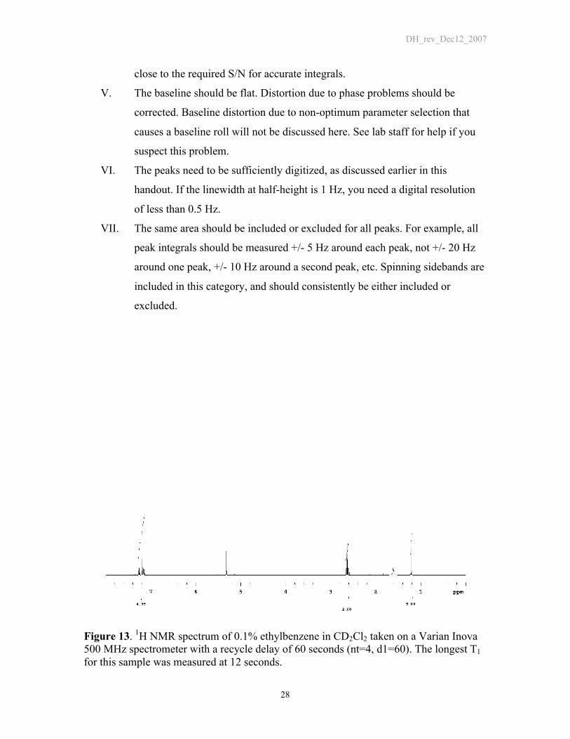
Figure 13. 1H NMR spectrum of 0.1% ethylbenzene in CD2Cl2 taken on a Varian Inova500 MHz spectrometer with a recycle delay of 60 seconds (nt=4, d1=60). The longest T1

for this sample was measured at 12 seconds.

DH_rev_Dec12_2007

29

With these points in mind, let’s take the 1H spectrum of ethylbenzene again. The

major factor for poor integration in Figure 12 was the difference in T1’s for the aromatic

protons (~12 seconds) and the aliphatic protons (~7 seconds). With no recycle delay,

there was not enough time to allow for complete relaxation. If we allow for complete

relaxation by setting d1 large enough, say 60 seconds, then integration becomes accurate

as shown in Figure 13 with only a 0.2% error of the aromatic protons.

Integration Take Home Lesson

Taken from Derome (p. 172)

“The moral of this section is that there are numerous contributions to the error in

a quantitative measurement made by FT NMR, and while each of them may be reduced to

1% or so in a practical fashion, the combined error is still likely to be significant. I am

always skeptical of measurements purporting to be accurate to better than a few percent

overall, unless they come with evidence that careful attention has been paid to the above

details.”

DH_rev_Dec12_2007

30

Homonuclear Decoupling

The purpose of this section of the handout is to explain what homonuclear

decoupling does. Examples of a homonuclear decoupled spectrum are given in Figure 14.

Homonuclear decoupling is a double-resonance technique that uses two RF fields to

affect magnetically active nuclei. Homonuclear decoupling involves applying a second

RF field to cause selective saturation of nucleus A while observing all other nuclei in the

Figure 14. Proton spectrum of 0.1% ethylbenzene in CDCl3 taken on a Varian Unity 400MHz spectrometer. The lower trace is the full, coupled spectrum. The upper inset showsthat by centering the decoupler on the triplet the quartet is collapsed to a singlet, whilethe lower inset demonstrates the effects of irradiating the quartet.

molecule; B, C, D, etc. If nucleus A is spin-coupled to nucleus B and if the second RF

field is strong enough, the result is that A is effectively prevented from spin-spin

interacting with B. The observed B nucleus spectrum will appear as if it is not coupled to

DH_rev_Dec12_2007

31

A. The A resonance commonly appears as a glitch as a result of this experiment. As

shown in Figure 14, if the triplet is homo-decoupled, the quartet collapses to a singlet.

Similarly, if the quartet is homo-decoupled, the triplet collapses to a singlet. You may

recall that a relatively high power, short RF pulse will have a frequency spread due to the

Heisenberg Uncertainty Principle; therefore, the second RF field used for the selective

decoupling will be lower power and have a longer duration.

Homonuclear Decoupling Take Home Lesson

Homonuclear decoupling is a fast and effective way to establish that two nuclei

are spin (scalar, ‘J’) coupled, and can be used to simplify a complex coupling pattern for

further analysis. It is also useful as a follow-up to a COSY experiment to confirm specific

couplings. To obtain definitive data the two signals must be separated by at least 0.5

ppm. It is also important to note that other signals close to the irradiation point may

experience a displacement in their chemical shift due to the decoupling field. This

displacement in the chemical shift is called a Bloch-Siegert shift and can be used to

measure the decoupling field strength.

DH_rev_Dec12_2007

32

Proton Decoupled 13C NMR spectra (13C-{1H})

The purpose of this section of the handout is to give you some useful information

about 13C-{1H} NMR spectroscopy. Since only about 1 in 100 carbon nuclei are NMR

active (1.10% are the NMR active 13C isotope), any means to improve S/N is essential.

Splitting of the 13C resonances as a result of coupling to attached protons will result in

decreased S/N and is, thus, undesirable. Therefore, 13C NMR spectra are typically run

proton decoupled. The symbol 13C-{1H} is used to denote this and implies the 13C

nucleus is observed while the proton nuclei are being irradiated, thus decoupling them

from the 13C nuclei. A typical 13C-{1H} spectrum (57% menthol in acetone-d6) is shown

in Figure 15.

Figure 15. A 13C-{1H} NMR spectrum of a 57% solution of menthol in acetone-d6

acquired on a Varian Unity 400 MHz spectrometer.

This is a double resonance experiment with the observed nucleus (13C) and

DH_rev_Dec12_2007

33

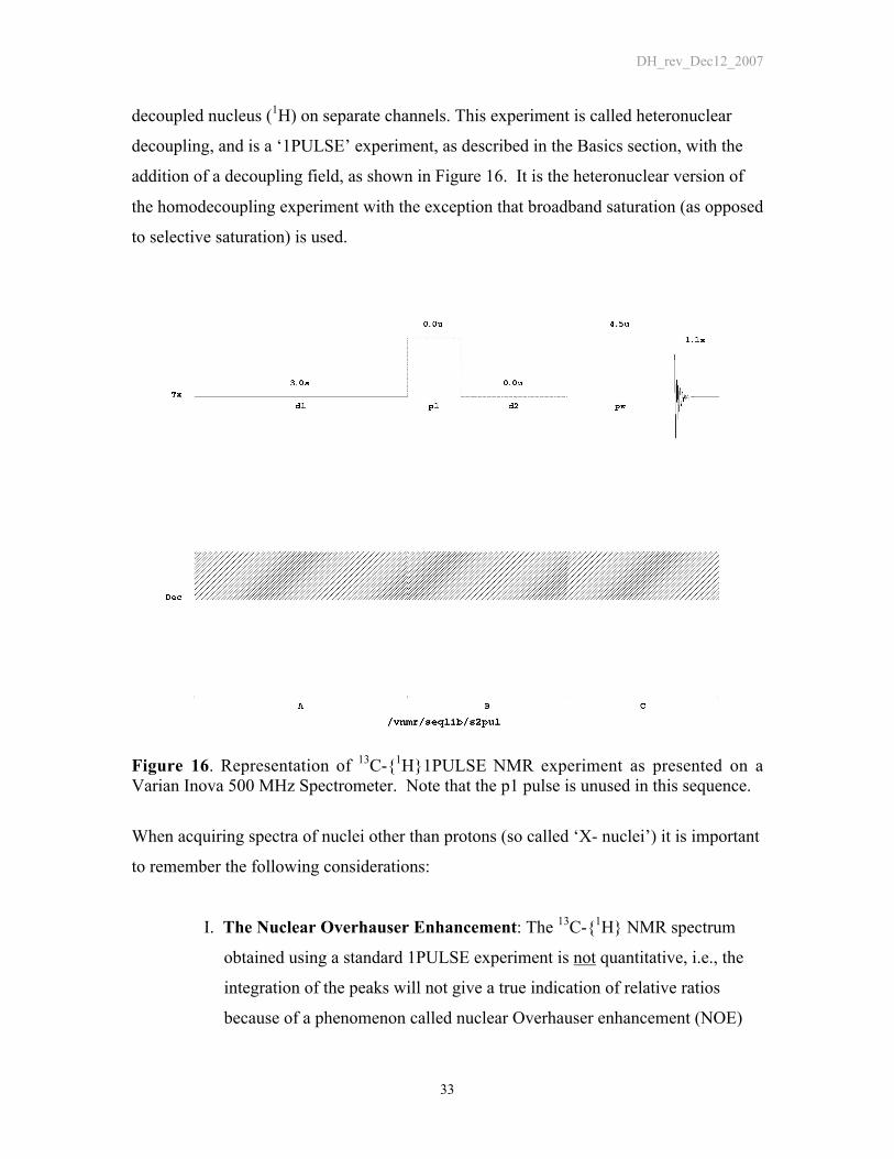
decoupled nucleus (1H) on separate channels. This experiment is called heteronuclear

decoupling, and is a ‘1PULSE’ experiment, as described in the Basics section, with the

addition of a decoupling field, as shown in Figure 16. It is the heteronuclear version of

the homodecoupling experiment with the exception that broadband saturation (as opposed

to selective saturation) is used.

Figure 16. Representation of 13C-{1H}1PULSE NMR experiment as presented on aVarian Inova 500 MHz Spectrometer. Note that the p1 pulse is unused in this sequence.

When acquiring spectra of nuclei other than protons (so called ‘X- nuclei’) it is important

to remember the following considerations:

I. The Nuclear Overhauser Enhancement: The 13C-{1H} NMR spectrum

obtained using a standard 1PULSE experiment is not quantitative, i.e., the

integration of the peaks will not give a true indication of relative ratios

because of a phenomenon called nuclear Overhauser enhancement (NOE)

DH_rev_Dec12_2007

34

arising from the continuous broad-band saturation of the protons. 13C nuclei

that have directly bonded protons can exhibit a signal enhancement of up to

1.98 (198%), or an almost threefold improvement in signal-to-noise. The

NOE is from the dipolar through-space coupling of the carbon and proton

nuclei and is dependent on many factors. Thus, the NOE will be different

for each unique carbon in a molecule. To obtain quantitative 13C-{1H}

spectra, you must do two things: follow the protocol given earlier on

integration, and carry out a ‘gated’ decoupling experiment, in which the

decoupler is gated on (turned on) during the acquisition time and gated off

(turned off) during the recycle delay. This is shown in Figure 17.

Figure 17. A gated decoupling pulse sequence for 13C-{1H} acquisition that has no nOeenhancement. Note that the decoupler channel (Dec) is only ‘on’ during segment C,which is the pulse and acquisition time. Compare to Figure 11.

The result of this experiment is a 13C-{1H} spectrum without NOE and is

necessary for obtaining quantitative 13C spectra.

DH_rev_Dec12_2007

35

II. T1 relaxation times: The Tl's of l3C nuclei are in general longer than those

found for protons, as shown below in Figure 18. Therefore, you may have to

wait very long times if you want accurate integrals from spectra. For

example, from Figure 18, quantitative integration of ethylbenzene would

require a total acquisition time (TT) of 5*36 seconds or 3 minutes per scan!

A paramagnetic relaxation agent such as Cr(acac) (available from Aldrich)

can be used to shorten the Tl's, but can sometimes be difficult to separate

from the compound. Note that the quaternary carbons have considerably

longer T1’s and, as a result, typically have much smaller signals than other

carbons.

CH2-CH3 CH3 NO2

(CH3-CH2-CH2-CH2)2

913

1336

14 7 16

3820

21

15

566.9

6.9

4.9

8.7 6.6 5.7 4.8

Figure 18. Examples of some representative 13C NMR T1 values, in seconds.

13C NMR Take Home Lesson

Obtaining useful 13C-{1H} spectra requires knowledge of the same basics as

needed for obtaining useful 1H spectra. When your spectrum doesn’t look right, you can

save frustration on the instrument be taking a quick spectrum of a 13C standard and

checking the S/N, or seeing if the standard is decoupled properly.

DH_rev_Dec12_2007

36

13C-{1H} DEPT Spectra

Distortionless Enhancement by Polarization Transfer (DEPT) is an experiment

that utilizes a polarization transfer from one nucleus to another, usually proton to carbon

or other X nucleus, to increase the signal strength of the X nucleus. DEPT is an example

of multi-pulse, multi-channel experiment, which uses synchronous pulses on two

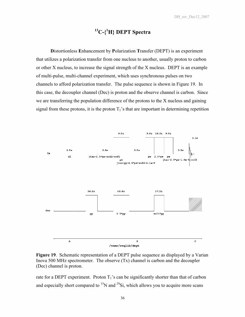
channels to afford polarization transfer. The pulse sequence is shown in Figure 19. In

this case, the decoupler channel (Dec) is proton and the observe channel is carbon. Since

we are transferring the population difference of the protons to the X nucleus and gaining

signal from these protons, it is the proton T1’s that are important in determining repetition

Figure 19. Schematic representation of a DEPT pulse sequence as displayed by a VarianInova 500 MHz spectrometer. The observe (Tx) channel is carbon and the decoupler(Dec) channel is proton.

rate for a DEPT experiment. Proton T1’s can be significantly shorter than that of carbon

and especially short compared to 15N and 29Si, which allows you to acquire more scans

DH_rev_Dec12_2007

37

per unit time than the X-{1H} experiment and thus obtain improved S/N. A further

advantage of this population transfer is the ability to perform multiplicity editing.

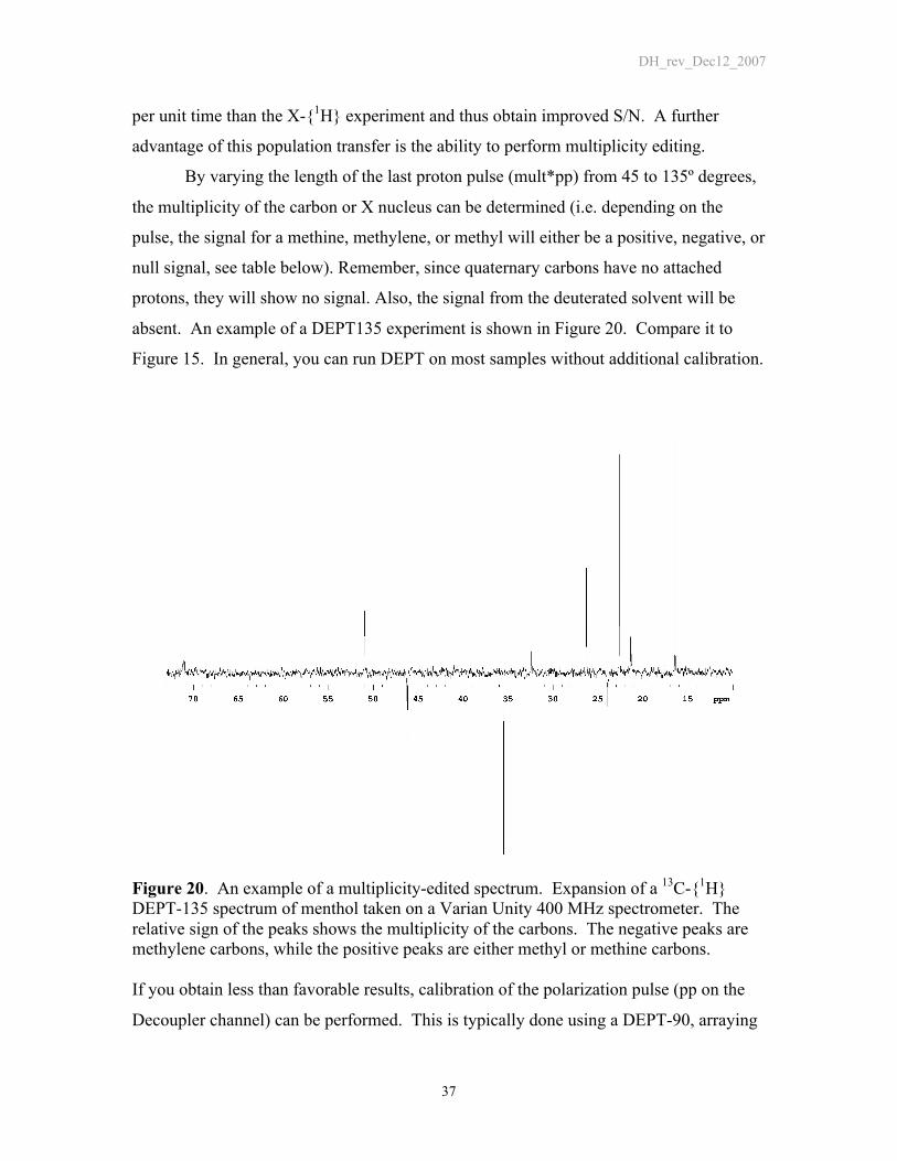
By varying the length of the last proton pulse (mult*pp) from 45 to 135º degrees,

the multiplicity of the carbon or X nucleus can be determined (i.e. depending on the

pulse, the signal for a methine, methylene, or methyl will either be a positive, negative, or

null signal, see table below). Remember, since quaternary carbons have no attached

protons, they will show no signal. Also, the signal from the deuterated solvent will be

absent. An example of a DEPT135 experiment is shown in Figure 20. Compare it to

Figure 15. In general, you can run DEPT on most samples without additional calibration.

Figure 20. An example of a multiplicity-edited spectrum. Expansion of a 13C-{1H}DEPT-135 spectrum of menthol taken on a Varian Unity 400 MHz spectrometer. Therelative sign of the peaks shows the multiplicity of the carbons. The negative peaks aremethylene carbons, while the positive peaks are either methyl or methine carbons.

If you obtain less than favorable results, calibration of the polarization pulse (pp on the

Decoupler channel) can be performed. This is typically done using a DEPT-90, arraying

DH_rev_Dec12_2007

38

pp, and looking for a maximum in the methine signal without contributions from other

carbons.

DEPT Take Home Lesson

DEPT is an effective means of determining 13C multiplicity that, when combined with

other NMR spectra and other experimental techniques (MS, FT-IR, etc.), can be an

invaluable tool for the analysis of unknown compounds.

Relative Intensities from DEPTPulse Angle (º) C (quaternary) CH (methine) CH2 (methylene) CH3 (methyl)

45 0 0.707 1 1.0690 0 1 0 0135 0 0.707 -1 1.06

DH_rev_Dec12_2007

39

Index:

AAcquisition Time (at), 2, 3, 4, 5, 7, 8, 9, 18, 19, 20, 23,

34, 35, 40Analog-to-digital converter (ADC), 6Apodization, 1, 21, 22, 23, 41

BBasics of FT NMR- Six Critical Parameters, 1, 3

CCarbon NMR, 32, 35Carbon NMR, factors affecting, 33Carbon NMR, pulse sequence, 33Carbon NMR, quantitative, 34

DDEPT, 2, 36, 37, 38DEPT, 135-, 37DEPT, relative intensities, 38Digital Resolution (res), 8, 18, 19, 20, 23, 28, 40

FFourier Transform, 2, 6, 7, 20Free-induction decay (FID), 4, 5, 6, 7, 14, 18, 19, 20,

21, 22, 23, 27, 40, 41

HHomonuclear Decoupling, 30, 31

IIntegration, 1, 9, 26, 29, 33, 35, 42Integration, factors affecting, 27Introduction, 1, 2

LLine-Shape, 1, 11, 13, 14, 17

NNuclear Overhauser Enhancement, NOE, 33, 34Number of Points (np), 3, 6, 7, 8, 20

PPeak Width at Half Height, 11, 12Pulse Width (pw), 3, 4, 9, 27

QQuiz, NMR, 2, 40

RRecycle Delay (d1), 3, 5, 8, 9, 26, 28, 29, 34

SShimming, 1, 13, 14, 16, 41Shimming, Figure, 16Signal-to-Noise (S/N), 3, 18, 19, 21, 22, 23, 24, 25,

27, 32, 34, 35, 37, 41Signal-to-Noise (S/N), calculation, 24Spectral Width (sw), 3, 7, 8, 27, 40Spectrometer Frequency, 3, 4, 6, 7, 8Spectrum Phase, 11, 12, 28, 41

TT1, longitudinal time constant, 9, 18, 26, 28, 29, 35,

36Table of Contents, 1Truncation Artifacts, 20

WWeighting, 1, 21, 22, 23, 41Weighting, Line Broadening, 22, 23, 24

ZZero-Filling, 1, 6, 8, 18, 19, 20, 23

DH_rev_Dec12_2007

40

NMR Basics Test

1. Diagram and label the three parts of the 1PULSE FT NMR experiment.

2. What is the result when you apply FT to a FID (time domain signal)?

3. What is the relationship between numbers of points, spectral width, acquisition time,

and digital resolution? What is the rule-of-thumb for adequate digital resolution? Which

of these parameters would you change if you wanted better digital resolution, and why?

4. What is the peak shape found in most solution NMR spectra?

DH_rev_Dec12_2007

41

5. What shim(s) should be adjusted if the peak shape is asymmetrically distorted?

6. What is the single best factor to tell whether a sample is poorly shimmed?

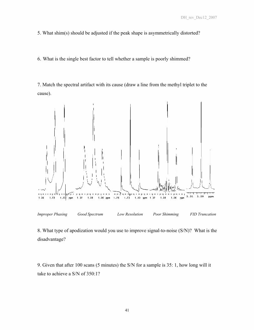
7. Match the spectral artifact with its cause (draw a line from the methyl triplet to the

cause).

Improper Phasing Good Spectrum Low Resolution Poor Shimming FID Truncation

8. What type of apodization would you use to improve signal-to-noise (S/N)? What is the

disadvantage?

9. Given that after 100 scans (5 minutes) the S/N for a sample is 35: 1, how long will it

take to achieve a S/N of 350:1?

DH_rev_Dec12_2007

42

10. What are the six factors that can affect the accuracy of a 1H NMR spectral

integration? Why? Are there any additional factors that affect the accuracy of 13C- {1H}

integration? Why?

11. Is there a difference between the 1PULSE FT NMR experiment used to acquire 13C-

{1H} NMR spectra and that used to acquire proton spectra? If yes, what is the difference?

12. For a DEPT135 spectrum, what are the relative intensities for the different

multiplicities of carbon?