© 2015 the aerospace corporation advances in dielectric property and thickness evaluation of...

© 2015 The Aerospace Corporation

Advances in Dielectric Property and Thickness Evaluation of Layered Composite Structures using Open-Ended Waveguides

Joseph (Toby) Case – The Aerospace CorporationSpace Materials Laboratory (SML), El Segundo, Los Angeles, CA 90250

M.T. Ghasr and Reza Zoughi – Missouri S&TApplied Microwave Nondestructive Testing Lab (amntl), Rolla, MO 65409

ISNDCM 2015June 23, 2015

[email protected]/MSD/ETG

AcknowledgementIR&D

Support from The Aerospace Corporation Independent Research and Development program is gratefully

acknowledged


IntroductionBackground and Contribution

• Microwave Material Characterization Techniques– Cavity– Transmission line– Free-space

• Far-field – Plane-wave / focused

• Near-field – open-ended rectangular waveguide and coaxial probes [1]

• Near-field open-ended rectangular waveguide– No need to cut and shape the sample– Requires a relatively large sample– Advanced flange designs to reduce reflection from flange [2]– Computationally Intense

[1] M.T. Ghasr, D. Simms, and R. Zoughi, "Multimodal Solution for a Waveguide Radiating Into Multilayered Structures—Dielectric Property and Thickness Evaluation," Instrumentation and Measurement, IEEE Transactions on, vol.58, no.5, pp.1505,1513, May 2009[2] M. Kempin, M.T. Ghasr, J.T. Case, and R. Zoughi, "Modified Waveguide Flange for Evaluation of Stratified Composites," Instrumentation and Measurement, IEEE Transactions on , vol.63, no.6, pp.1524,1534, June 2014


IntroductionExample Applications

Measure thickness and dielectric properties

. . .

Many Applications

TBCCorrosion

Under Paint


IntroductionContribution: Reduce Sources of Computational Complexity

• Forward problem– Evaluate reflection coefficient from a model– Adaptive segmentation

• Increase computational accuracy

• Reduce computational cost

• Inverse Problem– Determine a model from given reflection coefficient– Large quantity of degrees of freedom– Easily trapped in local minima– Significant reduction of the degrees of freedom using value relationships– Adaptive Segmentation reduces the likelihood of local minima and eliminates

solver “panic” (e.g., NaN or Inf)


Forward Problem [1]Challenges

• Large disparity (variation) in integrand value for low loss layers– Singularities for no-loss layers

• Gaussian Legendre integration is necessary but must have proper segmentation boundaries

• Segmentation is a function of layer properties and no direct relationship exists

• Main challenge: Where should integration samples be placed and with what concentration and with what weight?

[1] M.T. Ghasr, D. Simms, and R. Zoughi, "Multimodal Solution for a Waveguide Radiating Into Multilayered Structures—Dielectric Property and Thickness Evaluation," Instrumentation and Measurement, IEEE Transactions on, vol.58, no.5, pp.1505,1513, May 2009


Forward ProblemAdaptive Segmentation

1. Evenly distribute samples in one segment and evaluate integrand

2. Identify and locate peaks

3. Refine / solve for peak location (hill climbing / iterated local search)

4. Define segments using peak values as segment boundaries

5. Sample distribution– Evenly distributed between segments regardless of segment span– Steep integrands require more samples

• Demonstration comparing adaptive and primitive segmentation– Convergence Test

Segmentation Procedure


Air(1-j0.0001)

Forward ProblemComputational Example

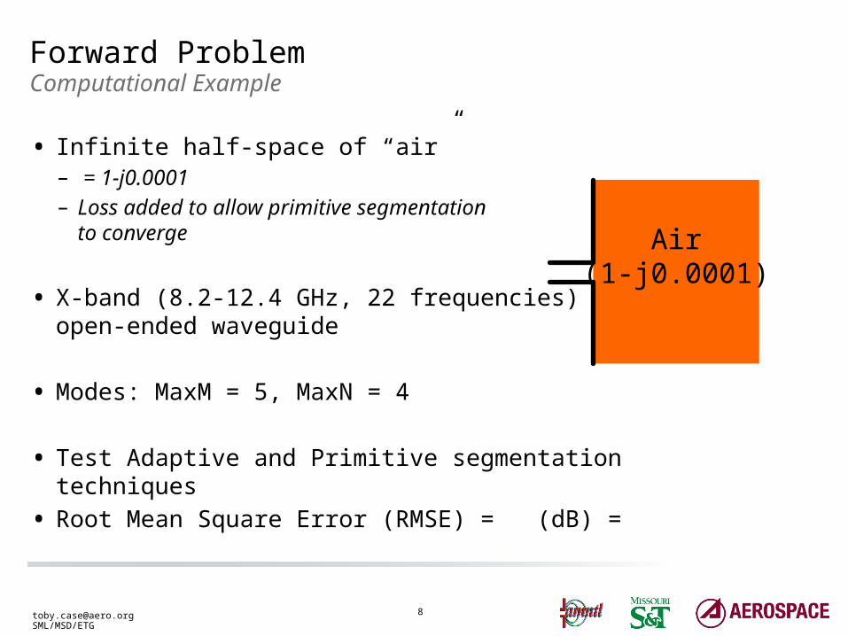
• Infinite half-space of “air”– = 1-j0.0001– Loss added to allow primitive segmentation

to converge

• X-band (8.2-12.4 GHz, 22 frequencies)open-ended waveguide

• Modes: MaxM = 5, MaxN = 4

• Test Adaptive and Primitive segmentation techniques

• Root Mean Square Error (RMSE) = (dB) =


Forward ProblemComputational Resource

Cisco UCS C460 M4• 4 x Intel Xeon E7-4850 v2 2.3GHz CPU

• 48 Cores / 96 Threads

• 1TB DDR3 memory

• 10GbE enabled

• CentOS 6.6

• Notes– It is a shared resource, times are approximate– Memory bottleneck due to other users– “nice” levels intentionally set to +5 (lower priority)


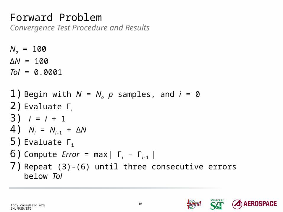
Forward ProblemConvergence Test Procedure and Results

No = 100

ΔN = 100

Tol = 0.0001

1) Begin with N = No ρ samples, and i = 0

2) Evaluate Γi3) i = i + 1

4) Ni = Ni-1 + ΔN

5) Evaluate Γi

6) Compute Error = max| Γi – Γi-1 |

7) Repeat (3)-(6) until three consecutive errors below Tol


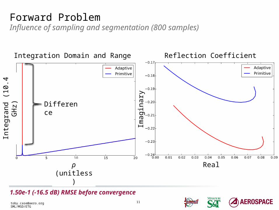
Forward ProblemInfluence of sampling and segmentation (800 samples)

1.50e-1 (-16.5 dB) RMSE before convergence

Imag

inar

y

Realρ (unitless)

Inte

gran

d (1

0.4

GH

z)

Difference

Integration Domain and Range Reflection Coefficient


Forward ProblemInfluence of sampling and segmentation (42500 samples, 1/4)

9.7e-3 (-40 dB) RMSE before convergence

Imag

inar

y

Realρ (unitless)

Inte

gran

d (1

0.4

GH

z)

Difference



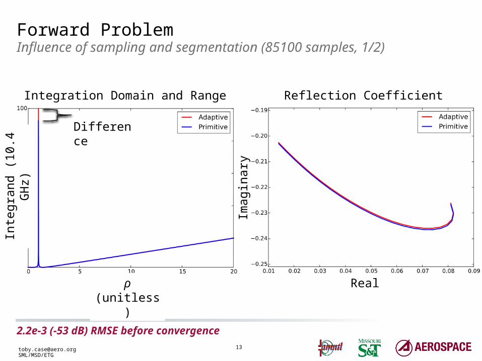
Forward ProblemInfluence of sampling and segmentation (85100 samples, 1/2)

2.2e-3 (-53 dB) RMSE before convergence

Imag

inar

y

Realρ (unitless)

Inte

gran

d (1

0.4

GH

z)

Difference



Forward ProblemInfluence of sampling and segmentation (170200 samples)

2.1e-4 (-74 dB) RMSE after convergence

Imag

inar

y

Realρ (unitless)

Difference

Inte

gran

d (1

0.4

GH

z)



Err

or (

dB)

N (samples)

Forward ProblemConvergence Test

Segmentation Number of Samples Time per freq. (sec)

Adaptive 800 0.38

Primitive 170200 560


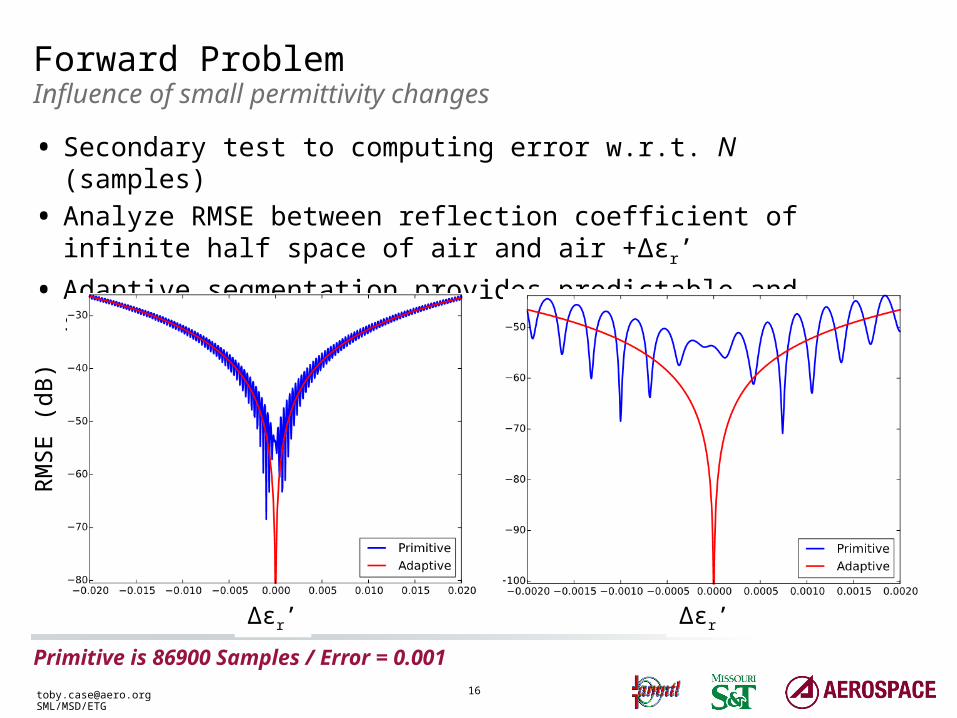
Forward ProblemInfluence of small permittivity changes

• Secondary test to computing error w.r.t. N (samples)

• Analyze RMSE between reflection coefficient of infinite half space of air and air +Δεrʹ

• Adaptive segmentation provides predictable and smooth variation

Primitive is 86900 Samples / Error = 0.001

RM

SE

(dB

)

Δεrʹ Δεrʹ


Inverse ProblemImprovements made to benefit the inverse problem

• Improvements to Forward Problem benefit Inverse Problem– Reduced computational cost

• Inversion is really forward-iterative– Improved computational accuracy

• Smooth solution space

• May use derivative based optimization methods

• Nearly eliminates bias to initial guess

• Reduce complexity of solution space by exploiting relationships– Every independent unknown is another dimension in the solution space– Further reduce chances of local minima– Exploit value relationships between electric and dimensional properties

• Direct – Values are identical

• Functional – Values are related by some function (e.g., curve fit)


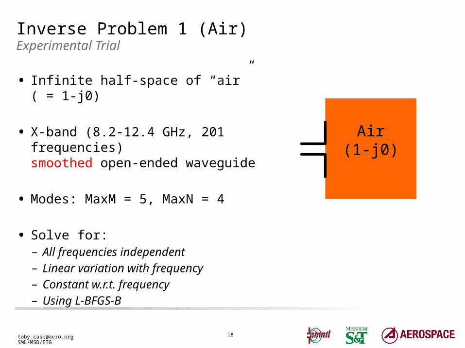
Air(1-j0)

Inverse Problem 1 (Air)Experimental Trial

• Infinite half-space of “air” ( = 1-j0)

• X-band (8.2-12.4 GHz, 201 frequencies)smoothed open-ended waveguide

• Modes: MaxM = 5, MaxN = 4

• Solve for:– All frequencies independent– Linear variation with frequency– Constant w.r.t. frequency– Using L-BFGS-B


Inverse Problem 1 (Air)Results

Relation RMSE RMSE (dB)

Relative Time

Theory 0.051 -25.9 -

Frequency 0.000 -172.0 x1

Linear 0.013 -37.7 x4

Constant 0.029 -30.8 x1

Freq (GHz)

ΓR

εrʹʹ

εrʹ ΓI


Inverse Problem 2Examples

Measure thickness and dielectric properties constant w.r.t. frequency

Label εrʹ - Permittivity εrʹʹ - Loss Thickness (mil)

Air 1 0.0000 4

Rogers TMM10i 9.9 0.0198 20

Air 1 0.0000 4

Rogers R04533 3.33 0.0083 60

Air 1 0.0000 N/A

Rogers R

Rogers T

Air


Inverse Problem (Layers)Results – Constant w.r.t. Frequency

Reduced performs similarly numerically, but ~2x faster

Item Theory All Independent Reduced

Dimensions N/A 14 10

RMSE (dB) -35 -44 -44

Air - εrʹ 1.00 1.011±0.012 1.027

Air - εrʹʹ 0.0 (2.8±3.9)e-4 0.0

Rogers T - εrʹ 9.9 9.9 9.9

Rogers T - εrʹʹ 0.0198 0.0230 0.0233

Rogers T – Thk (mil) 20 20.75 20.63

Rogers R - εrʹ 3.330 3.339 3.339

Rogers R - εrʹʹ 0.0083 0.0147 0.0154

Rogers R – Thk (mil) 60 61.16 61.14


Summary / ConclusionRemarks

• Forward Problem– Adaptive segmentation is the only appropriate segmentation– More accurate and faster results

• Inverse Problem– Solution is largely dependent upon the accuracy of the forward problem

and the number of unknowns– Reduce unknowns wherever possible (i.e., make overdetermined)

• Questions?


Forward ProblemHill Climbing

1. i = 0, Δi = Δρ/2, ρi = ρo, Vi = V(ρo)

2. i = i +1

3. ρi = ρi-1+ Δi-1

4. Vi = V(ρi)

5. If Vi > Vi-1, then Δi = Δi-1/2

6. If Vi < Vi-1, then Δi = -Δi-1/2, ρi = ρi-17. Repeat (2)-(6) until Δi < Tol

Variable Description

Δρ Current ρ sampling

i Iteration

Δi Current increment

ρi Current position

Vi Current Value

© 2015 the aerospace corporation advances in dielectric property and thickness evaluation of...

Documents

acknowledged slide

paint slide

inf slide

waveguide radiating

model adaptive segmentation

modified waveguide flange

ieee transactions

aerospace corporation