"

.'

Pacific Marine Sci~nce ReP9~t

PRACTICAL ACCURACY OF SIPPICAN T-7 XBTs

by

Wayne Wood

Institute of Ocean Sciences, Patricia Bay

Victoria, B.C.

October 1976

This is a manuscript which has received only limited

circulation. On citing this report in a bibliography,

the title should be followed by the words "UNPUBLISHED

MANUSCRIPT" which is in accordance with accepted bib­

liographic custom.

1

In an effort to determine the practical accuracy, precision, and reliability of Sippican Corporation T-7 expendable bathythermographs used with a Sippican MK 28-3 recorder plotter, XBT profiles were taken immediately after STD casts during an August 1975 cruise in the North­eastern Pacific Ocean. The data obtained was then used to compute the mean (STD- XBT) temperature difference (accuracy), the standard deviation of these differences (precision), and the probability (expressed as a percent­age) that an individual XBT will produce a usable trace (reliability). The effects of various sources of error are considered, including thermistor accuracy, digitizing errors, and errors in the probe fall rate .

During the cruise 102 XBT casts were made, 8 of which were obvious rejects appearing to be caused by leakage problems in the cable and are not considered here. In these cases another XBT was launched and the trace redone. Of the 94 usable traces 64 had corresponding sm traces taken within 40 minutes at the same position using a Gui1d1ine model 8700 CTD probe with a Gui1dline model 87121 deck unit and a Hewlett Packard model 7046A chart recorder. Both XBT and STD traces were digitized using a Hewlett Packard model 9864A digitizing table with a resolution of 0.01* inches (0.025 cm).

In sm traces the effects of digitizing errors were small as the temperature and depth scales used were large relative to the trace thickness and digitizing resolution. The trace width of ~ 1mm made it easy to fellow with the digitizer. Digitizing errors for sm traces are considered to be < ±0.02°C based on trace scale and digitizer resolution. XBT traces however, have confined temperature and depth scales (2°C/cm, 38 meters/cm). To compensate for this a thin trace is used which is ' difficult to digitize. A slight variation from the trace with the digitizer can cause an error of ±O.l °C. The resolution of the digitizer corresponds to 0.05°C on the XBT scale. Also, in XBT traces, the trace had to be made heavier, using a pencil, to make it readily visible, contributing further to the errors.

An XBT trace was digitized 10 times to estimate the errors due to digitizing technique. An average difference of 0.05°C was found among the 10 temperature values at any depth. This is comparable to the resolution of the digitizer which on the XBT scale corresponds to 0.05°C. The standard deviation from this mean was 0.14°C. In view of this, digitizing of XBT traces would probably not give any more accuracy than reading the traces by sight .

Histograms of the (STD-XBT) temperature differences were plotted for the depths 0, 10, 100, 250, SOD, and 600 meters, these are shown in Figure 1. The mean and standard deviation of these differences are given in Table I. STD's have been assumed correct as comparison with Nansen bottle casts showed the average, low gradient (approximately 0.03°C/10m), variation was < ± 0.02°C.

* Manufacturer's specification

Depth Om

X -0.164°C

SD 0.143°C

N 64

(In view of the

2

TABLE I

Mean (X) and Standard Deviation (SD) of Temperature Differences (STD-XBT) at Selected Depths

10 m 100 m 250 m 500 m 600 m All

-0.ll4°C 0.034°C 0.034°C -0.021 °c -0.029°C -0.059°C

0.23l oC 0 . 221°C 0.22loC 0.210 oe 0 .165°C 0.2l6°C

64 64 64 62 62 380

manufacturer's specifications for thermistor accuracy the last 2 digits are not significant.)

Most of the temperature differences are <± 0.15'C. The remainder havebeen split into two groups ± 0.20°C+±0.30°C and ~± 0.35°C . The percent­age falling into each group for the 6 depths used is shown in Table II. For the two larger temperature difference ranges the individual consecutive STD and XBT numbers have also been listed along with symbols representing possible reasons for their larger differences. Sample traces showing the categories "erratic start" and "other unusual appearances 11 are given in Figures 2, 3, 4. In some cases reexamination of the original traces revealed errors made in the original digitizing.

3

TABLE II

Percentage of Traces Falling Into The 3 Groups of Agreement {<± 0.15°C; ± 0.20°C+± 0.30°C; ~ 0.35°C}

Depth STD-XBT Differences (% of 64) (Trace # given is STD #/XBT #)

Meters <± 0.15°C

o 66% 28% trace numbers 6% trace numbers

6/6 24/36 * 58/65 a 72/82 17/22 a 11/12 a 26/39 a+ 65/76 75/85 a 51/60 + 15/20 42/46 a 67/78 83/93 70/80 * 20/28 a 53/62 a 69/79 + 80/90 22/32 56/63 + 71/81

10 81% 13% 6%

6/6 15/20 49/56 a 53/62 17/22 a 26/39 a 11/12 a 22/32 + 51/60 + 83/93 + 20/28 a 61/71 a

100 75% 17% 8%

4/3 + 20/28 a 53/62 72/82 + 17/22 a 24/36 + 12/14 44/47 * 67/78 + 75/85 a 18/24 a 59/67 + 19/26 49/56 a 69/79 * 23/34 + 5/4

250 90% 6% 4%

17/22 a 67/78 t:> 69/79 t:> 76/86 * 18/24 at:> 5/4

500 87% 11% 2%

4/3 * 18/24 a 25/38 62/73 t:> 5/4 17/22 a 22/32 * 59/67 *

600 93% 5% 2%

117/22 a 62/73 t:> 76/86 * 5/4

* = Digitizing Error (XBT) + = Large Gradients Present (re: STD cast), ±10 meters of depth considered,

gradients ~.l°C/m

a Erratic Start at beginning of trace (XBT) t:> = Other unusual appearances to the trace (XBT)

4

If all trace comparisons with digitizing errors, lIerratic starts", and "other unusual appearances" noticed upon closer inspection are omitted the results then become as in Table III.

Depth

0 10

100 2S0 SOO 600

TABLE III

Tables I and II Combined, With Digitizing Errors, "Erratic Starts", and "Other Strange Appearances" P~emoved

<± O.lSoe (± 0.20 oe+± 0.30 0 e) >± 0.3Soe X SD

80% 16% 4% - O.13°e -O.lOoe 92% 8% - 0.04°e 0.09°e 83% ll% 6% O.Oloe 0.18°e 98% 2% O.Oloe O.lOoe 96% 2% 2% o.oooe 0.08°e 98% 2% -O.Oloe 0.07°e

N

S4 57 57 57 55 58

In a few cases the STD traces showed large temperature gradients at one or more of the shallower depths. Since a time interval of 30 to 40 minutes usually elapsed between the STD and XBT tracings, which is comparable to the Brunt-Vaisala frequency at these depths, apparent temperature differences may be actually due to vertical motion of the isotherms rather than a fault of the XBT. If these are eliminated, the results become as in Table IV.

TABLE IV

Table III With Gradient Data Removed

Depth <± O.lSoe (± 0.20 oe+± 0.30 0 e) >± 0.35°e X SD N

0 85% 13% 2% - 0.12°e 0.09°e 51 10 96% 4% - 0.04°e 0.08°e

100 92% 6% 2% O.Oloe 0.12°e 51 250 98% 2% O.Oloe O.lOoe 57 SOO 96% 2% 2% o.oooe 0.08°e 55 600 98% 2% -O.Oloe 0.07°e 58

5

As is evident from Tables II and III gradient effects at depths of 250, 500, and 600 meters are small. Errors at these depths are mainly due to thermistor accuracy, digitizing, and the assumed fall rate of the probe. For shallower depths vertical gradients are such that it is possible to plot standard deviations of isothermal (STD-XBT) depth differences as a function of mean isothermal depth with the results shown in Table V and Figure 5. The plot in Figure 5 is linear with a slope of 0.03 (meters) standard deviation/meter, and a 0 depth intercept of 3.5 (meters) standard deviation. Surface wave motion (typically 3m peak to trough height) may account for a part of the non zero intercept. XBT digitizing inaccuracies could account for almost half of the intercept value. Variations in probe fall velocity would account for the linearity in Figure 5 as depth is determined by velocity assumed/time elapsed.

Let Va assumed velocity VR = real velocity Da = assumed depth Dr real depth t time

then

Dr-Da (Vr-Va)t (Vr-Va)Dr/Vr

or

Dr-Da = Constant x Dr

The mean (STD-XBT) differences being quite small would imply the best average values available for probe fall rate and change in depth scale with inceasing depth (to account for pressure effects) had been chosen. Variation between actual and assumed fall velocities needed to produce the slope of Figure 5 is about 3% for an assumed fall velocity of approximately Bm/s (from manufacturer's specifications).

Isotherm

6

TABLE V

Comparison of STD and XBT depth values for the 5°C, 6°C, and 10°C isotherms

Depths All depths <150m only

(meters) (meters)

X -0.92 -0.92 STD-XBT SD 4.53 4.53

N 60 60 Mean Depth* 35 35 SD (depth) 6 6

X 0.28 -1.00 STD-XBT SD 7.96 6.15

N 58 28 Mean Depth* 143 56 SD (depth) 77 38

X 3.49 1.23 STD-XBT SD 10.81 5.39

N 57 13 Mean Depth* 245 76 SD (depth) III 12

Depths :.150m only

(meters)

2.50 10.68 30

210 32

4.66 11.15 44

295 70

*In each case the Mean Depth is the mean of the N depths used in any category.

In order to assess the probability of obtaining a reasonably correct temperature value at a particular depth cases where the fault was in the digitizing, gradients, or time interval between STD and XBT casts may be eliminated with the results shown in Table VI.

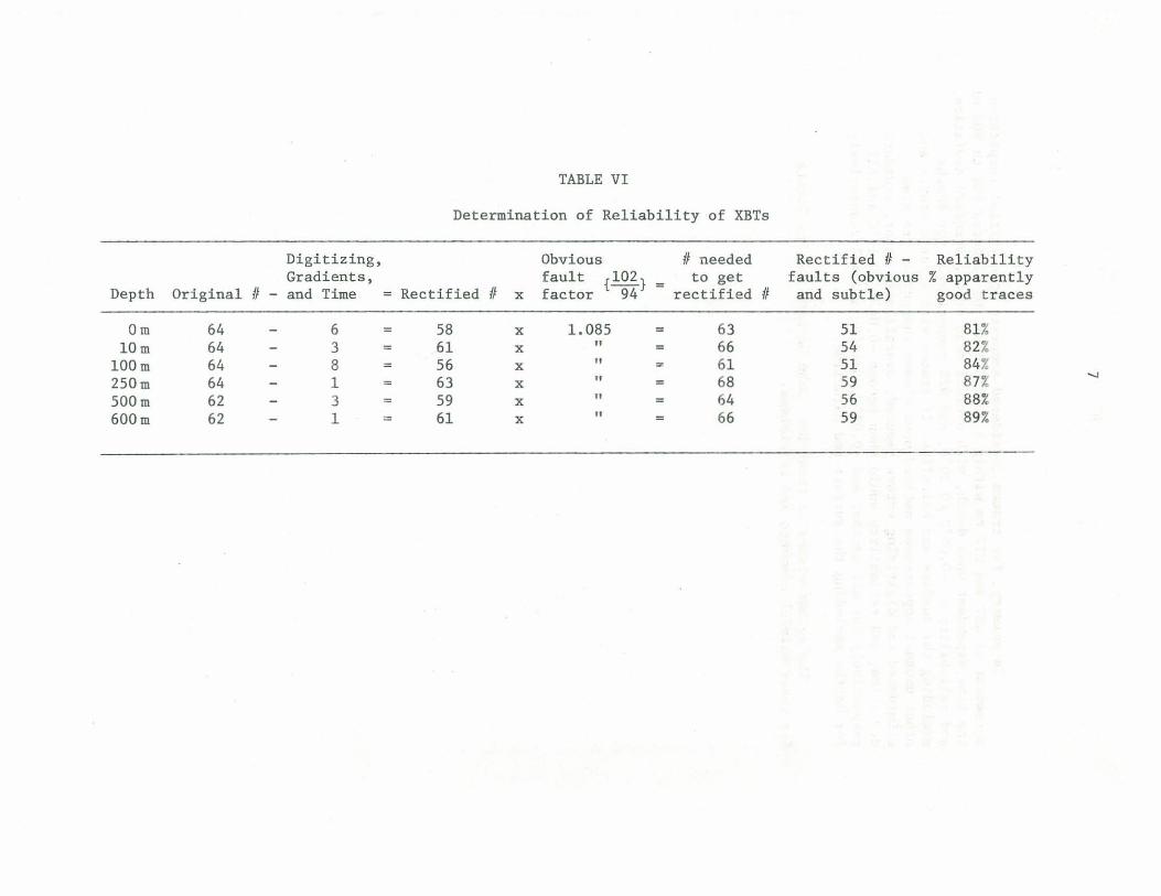
TABLE VI

Determination of Reliability of XBTs

Digitizing, Obvious II needed Rectified II - Reliability Gradients, fault {102} to get faults (obvious % apparently

Depth Original II - and Time Rectified II x factor 94 rectified II and subtle) good traces

Om 64 6 58 x 1.085 63 51 81% 10m 64 3 61 x n = 66 54 82%

100m 64 8 = 56 x n ~ 61 51 84%

250m 64 1 63 n 68 59 87% .... x

500m 62 3 = 59 x n 64 56 88% 600m 62 1 = 61 x n 66 59 89%

8

In summary, for traces considered accurate upon initial inspection agreement of XBT and STD to within ± O.ISDC could be expected 80% to 90% of the time dependent upon depth, with overall mean error, standard deviation, and reliability of -O.OSDC~0.20°C, and 92% respectively for depths excluding the surface and halocline. If traces with erratic starts and other unusual appearances noticed upon closer inspection are also eliminated and digitizing errors reduced, overall mean error, standard deviation, and reliability would then become -0.04 DC,;0.17 DC and 81% respectively for all depths; and -0.02DC,~O.IODC. and 87% respectively for depths excluding the surface and halocline.

The author wishes to thank Drs. John Garrett and Sus Tabata for their helpful comments and criticisms.

Figure l(a)

20

16

12

• 4

o

20

11>1.

'" ~ or 1-12

4

o

20

IS

12

• 4

o

9

o METERS

I I I I I" r:t ... ":2 0 .2 .~ -.6

10 METERS

I I II Fi ... ~2 .2 ~ '.S

10 0 METERS

,

I " ,III, I I I I I I

<:S ~5 c:;r:J -.2 -.1 0 .I .2.:! · ~ ·.!I'.s STD -XBT difference ·C

Histograms of (STD-XBT) temperature differences for depths o m, 10 m, and 100 m.

Figure l (b)

10

20 2 !iO METERS

I. 12

•

o I I II I, 4

r:· -~ ,2 .2 ~ ' .. 2 0

soo METERS

• 2

• 4

0 I I, II I .~ -~ -.2 .2 .. ' ' ..

!C, 2 6 00 METERS

I.

12

• 4 -

Hi sto grams of (STD-XBT) temperature differences for depths 250 m, 500 m, and 600 m.

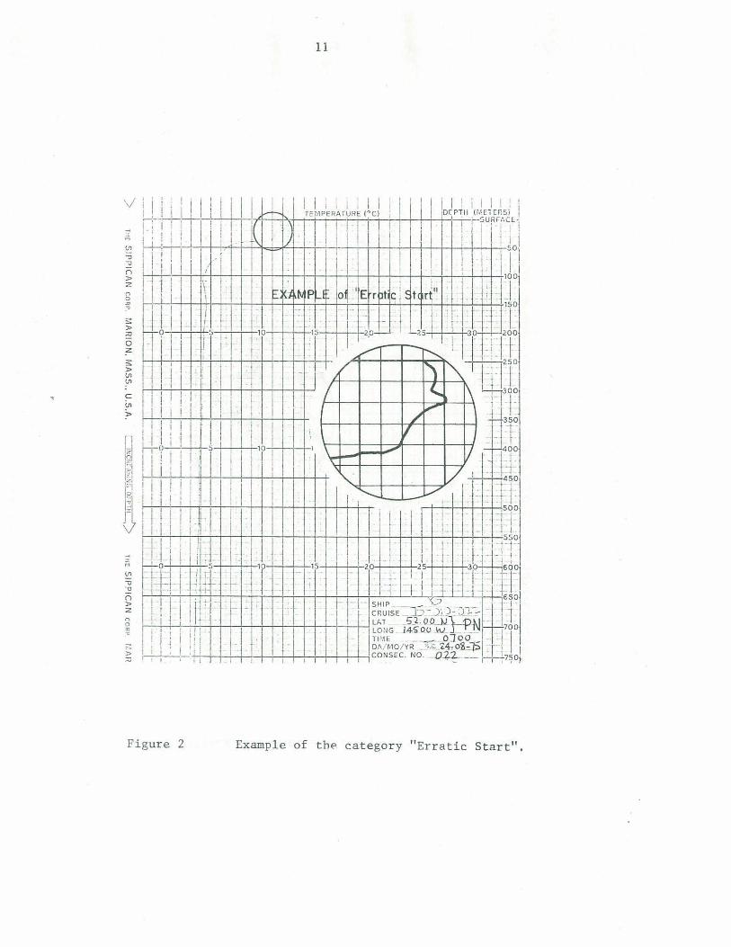
11

Figure 2 Example of th" category "Erratic Start".

12

Figure 3 Example of the category "Erratic Start".

Figure 4

13

Example of the categories "Erratic Start" and "Other unusual Appearances l1

•

,.... I­m x I 14 o Ii; v

z 12 o ti GjIO o

o It:: C§ 8 z i! II) 6 :t: Ii: ILl o 4

2

Figure 5

14

SLOPE = .03m SO/m

50 100 200 MEAN DEPTH

300 meters

Standard deviation of (STD-XBT) depth differences plotted as a function of depth.