zwick center for food and resource policy - cag.uconn.edu · zwick center for food and resource...

1

Zwick Center for Food and Resource Policy

Working Papers Series

No. 14

Uniform Price Mechanisms for Threshold Public Goods Provision:

An Experimental Investigation

Zhi Li*, Christopher Anderson* and Stephen Swallow**

November 1, 2012

Department of Agricultural and Resource Economics College of Agriculture and Natural Resources

1376 Storrs Road, Unit 4021 Storrs, CT 06269-4021 Phone: (860) 486-1927

Contact:

[email protected]

* School of Aquatic and Fishery Sciences, University of Washington ** Department of Agricultural and Resource Economics, University of Connecticut This work was possible thanks to substantial funding from USDA/NIFA/AFRI award 2009-55401-20050, with supplemental assistance from a USDA/NRCS/Conservation Innovation Grant; the University of Rhode Island and University of Connecticut Agricultural Experiment Stations, and the DelFavero Faculty Fellowship.

2

Research Highlights:

We introduce two novel “uniform price” mechanisms for provision point public goods We compare them to proportional rebate (PR) and provision point (PPM) mechanisms Mechanisms are evaluated with heterogeneous values and a range of provision points Our novel mechanisms generate higher contributions than PR and PPM. Differences in contribution behavior are explained by the marginal penalty structure.

Abstract

This paper introduces two new mechanisms for provision point public goods, motivated by the design of uniform price auctions: the uniform price auction mechanism (UPA) collects an endogenously determined uniform price from everyone offering at least that price, while the uniform price cap mechanism (UPC) collects the uniform price from everyone offering at least that price, plus the full offer of everyone offering less. UPA and UPC are compared with the provision point mechanism (PPM) and the proportional rebate mechanism (PR). We use undominated perfect equilibrium and the marginal penalty associated with overcontribution to provide benchmark predictions for an experimental comparison with heterogeneous induced values, and with different provision point treatments. We find UPA generates by far the highest group and individual contributions at all provision points and values, but has the lowest provision rate; UPC elicits higher aggregate contributions than PPM and PR, and has the highest provision rate, driven by higher contributions from high-value individuals, especially at moderate provision points. This is consistent with subjects offering more in mechanisms with lower expected marginal penalty, but the effect is most significant when marginal contributions are more likely to affect provision.

Keywords: Uniform price auction, Uniform price cap, Proportional rebate, No rebate

• We introduce two novel “uniform price” mechanisms for provision point public goods

• We compare them to proportional rebate (PR) and provision point (PPM) mechansims

• Mechanisms are evaluated with heterogeneous values and a range of provision points

• Our novel mechanisms generate higher contributions than PR and PPM.

• Differences in contribution behavior are explained by the marginal penalty structure.

3

1. Introduction

A provision point public good is one that can be provided only when a threshold level of funding

contributions is met. Canonical examples include bridges, parks and schools that require a

particular amount of funding to be built, and realistic examples include public radio broadcasting,

hospital and university buildings, and environmental conservation projects to which people

actually make contributions. The public goods literature typically envisions determining

outcomes through the provision point mechanism (PPM), in which people voluntarily and

simultaneously contribute toward funding the good; if the total contribution reaches or exceeds

the cost (provision point or threshold), the good is provided; otherwise contributions are

refunded (money back guarantee). Because it is simpler than other public goods mechanisms

with an interior Nash equilibrium that supports provision—in contrast to the unique zero-

contribution prediction of the voluntary contribution mechanism—PPM has been systematically

studied, both theoretically1 and experimentally.2

The presence of a provision point has induced an additional literature on how to rebate

contributions in excess of the provision cost, and how the rebate rules affect incentives for

making contributions. Marks and Croson (1998) compare no-rebate, proportional rebate (PR),

and utilization rebate, and find a utilization rebate leads to higher contributions, but no

significant difference between no-rebate and PR under complete information; while Gailmard

and Palfrey (2005) find PR (called PCS in their paper) induces significantly higher contributions

than no-rebate when value is private information. However, only a few of the possible factors

affecting contributions have been explored. Rondeau et al. (1999) assessed the group size effect

and information (about group size and provision point) effects in PR; Rondeau et al. (2005)

compared PR with the voluntary contribution mechanism; and Spencer et al. (2009) compared

PR and five other rebate rules in one-shot games. Therefore, in introducing two novel

mechansims, this paper extends our understanding of how rebate rules affect the contribution

levels as private value and relative provision point change.

1 Bagnoli and Lipman (1989) study PPM under complete information; Nitzan and Romano (1990), McBride (2006), and Barbieri and Malueg (2010a) discuss threshold uncertainty; Alboth et al. (2001), Menezes et al. (2001), Laussel and Palfrey (2003), and Barbieri and Malueg (2008, 2010b) discuss PPM with private value information. 2 See Chen (2008) for a recent review of related experimental studies; for earlier reviews see Davis and Holt (1993) and Ledyard (1995).

4

Our novel mechanisms are motivated by payment rules in multi-unit uniform price auctions. In

our uniform price auction mechanism (UPA), everyone who pays, pays the same price: if there

exists a price such that the number of contributions at or above that price multiplied by the price

equals the provision point, then the good is provided, with only those offering at or above the

uniform price paying the uniform price; the lowest such price will be chosen if more than one

uniform price is possible. Our second mechanism addresses the inefficiency inherent in UPA,

that contributions can exceed the provision cost, but still no uniform price meeting the provision

rule exists. In the uniform price cap mechanism (UPC), no one pays more than the uniform price:

if the provision point is exceeded, the lowest price cap will be calculated so whomever

contributes above the cap only pays the cap, and those contributing less than the cap pay their

full offer, such that the final collected payments equal the provision point.

The intuitive motivation for these mechanisms is fairness, in the sense that high contributors are

not penalized by being required to make higher payments, and contributors with low values not

penalized by offering a greater portion of their value, unless their money is absolutely needed for

provision. Thus, when public good benefits are heterogeneous, the high value people sensitive to

distributional considerations might contribute more in UPA and UPC than in PPM and PR, since

their additional contributions might not be needed; they improve the likelihood of provision if

they are.

Even in the absence of strong other-regarding preferences, the rebate rules in UPA and UPC

have different marginal penalty structures from PPM and PR, and hence could induce different

contribution levels. Marginal penalty, as used by Marks and Croson (1998), describes the cost of

contributing an additional dollar conditioned on provision, which differentiates among rebate

rules since it essentially captures how extra money is returned. For example, PPM has a

marginal penalty of -1 since there is no rebate, and the marginal penalty in PR is, in general,

between -1 and 0. Intuitively, in an environment with value or strategic uncertainty, the lower

the marginal penalty of contribution, the higher the potential contribution and the higher the

likelihood of provision. However, when comparing PPM and PR, Marks and Croson (1998) and

Gailmard and Palfrey (2005) find mixed results, indicating that the effects of marginal penalty

need further investigation. The ranges of contributions with zero marginal penalty in UPA and

5

UPC extend the range of observable marginal penalties beyond those achievable with PPM and

PR, and can provide more insights about the conditions under which agents can be induced to

make higher offers in support of public goods.

Uniform price auctions have been widely studied in application to the private supply for public

resources (e.g., Cason and Gangadharan, 2004, 2005; Jack et al., 2009; Evans et al., 2009), but

not in provision applications of private demand. Gailmard and Palfrey (2005) apply uniform

price auctions to excludable public goods, or club goods, leading to a fundamentally different

implementation of the auction. Like this paper, they use heterogeneous values with incomplete

information, which also extends the standard public good environments. Marks and Croson

(1998) use homogeneous induced values under complete information, and Rondeau et al. (1999)

and Spencer et al. (2009) use heterogeneous values but only in one-shot games.

The rest of the paper is organized as follows. Section 2 defines precisely the four mechanisms to

be compared. Section 3 characterizes the mechanisms’ undominated perfect Nash equilibria, and

their respsective marginal penalty structures. Section 4 describes the experimental design and

procedures. Sections 5 and 6 discuss the observed aggregate and individual contributions.

Section 7 synthesizes these results.

2. The Mechanisms

Consider a group of size N, in which each subject is endowed with the same initial monetary

fund I. Each subject simultaneously chooses to contribute a ci to the provision of a threshold

public good with the cost of PP (provision point), and how much I - ci to keep for themselves. If

the public good is provided, each subject receives a private value of vi, which is the individual-

specific benefit from the public good. If the public good is not provided, all contributions are

refunded (money-back guarantee).

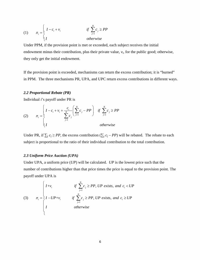
2.1 Provision Point Mechanism (PPM)

The payoff function for subject i under PPM is

6

(1) 1

N

i i jji

I c v if c PP

I otherwiseπ =

− + ≥=

∑

Under PPM, if the provision point is met or exceeded, each subject receives the initial

endowment minus their contribution, plus their private value, vi, for the public good; otherwise,

they only get the initial endowment.

If the provision point is exceeded, mechanisms can return the excess contribution; it is “burned”

in PPM. The three mechanisms PR, UPA, and UPC return excess contributions in different ways.

2.2 Proportional Rebate (PR)

Individual i’s payoff under PR is

(2) 1 1

1

N Ni

i i j jNj j

jij

cI c v c PP if c PPc

I otherwise

π = =

=

− + + − ≥ =

∑ ∑∑

Under PR, if ∑j cj ≥ PP, the excess contribution (∑j cj – PP) will be rebated. The rebate to each

subject is proportional to the ratio of their individual contribution to the total contribution.

2.3 Uniform Price Auction (UPA)

Under UPA, a uniform price (UP) will be calculated. UP is the lowest price such that the

number of contributions higher than that price times the price is equal to the provision point. The

payoff under UPA is

(3)

1

1

+ , ,

+ , ,

π

=

=

≥ <

= − ≥ ≥

∑

∑

N

i j ij

N

i i j ij

I v if c PP UP exists and c UP

I UP v if c PP UP exists and c UP

I otherwise

7

. If a subject contributes less than UP, the

subject pays nothing and all the contribution will be rebated. If a subject contributes UP or more,

the subject will pay only the price UP and the excess contribution will be rebated.

It should be noted that to provide the good, UPA requires not only that the total contribution

meet or exceed PP, but also that the number of relatively high individual contributions be

sufficient. More precisely, PP and the group size together determine a set of at most N possible

prices, where PP is shared by n≤N individuals offering at least PP/n. If the individual

contributions exceed PP, but cannot satisfy np=PP, the good cannot be provided even when

contributions offered meet or exceed PP.

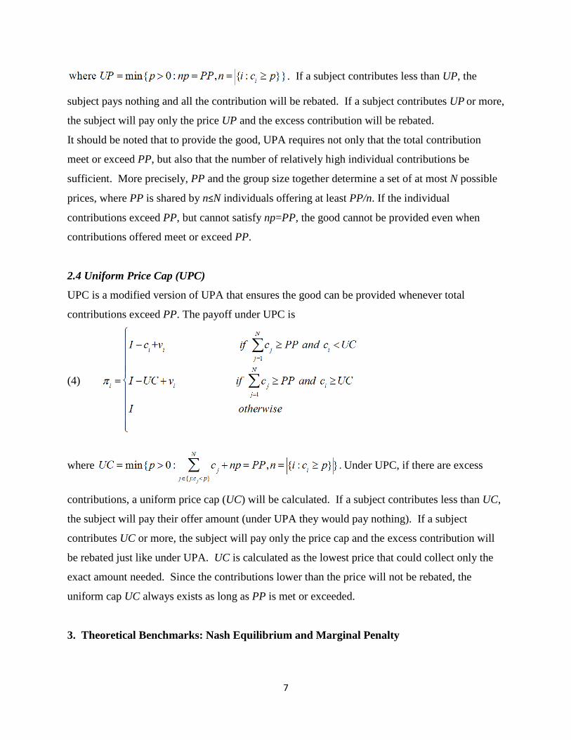
2.4 Uniform Price Cap (UPC)

UPC is a modified version of UPA that ensures the good can be provided whenever total

contributions exceed PP. The payoff under UPC is

(4)

where . Under UPC, if there are excess

contributions, a uniform price cap (UC) will be calculated. If a subject contributes less than UC,

the subject will pay their offer amount (under UPA they would pay nothing). If a subject

contributes UC or more, the subject will pay only the price cap and the excess contribution will

be rebated just like under UPA. UC is calculated as the lowest price that could collect only the

exact amount needed. Since the contributions lower than the price will not be rebated, the

uniform cap UC always exists as long as PP is met or exceeded.

3. Theoretical Benchmarks: Nash Equilibrium and Marginal Penalty

8

To predict how the four mechanisms will lead to different individual and aggregate contributions,

we use undominated perfect equilibrium (UPE) and the marginal penalty associated with

contribution beyond the provision point as theoretical benchmarks. UPE makes a precise

prediction about aggregate contributions, but includes a broad continuum of equilibria leading to

that aggregate. We use marginal penalty to understand patterns of disequilibrium, which may be

interpreted as a (non-refinement) selection process among UPE.

3.1 Undominated Perfect Equilibrium

Bagnoli and Lipman (1989) show that the undominated perfect equilibria (UPE)3

of PPM with

complete information lead to Pareto efficient Nash equilibrium outcomes, wherein the provision

point is exactly met and no one contributes more than their value, vi. They also argue that, when

rebate rules are incorporated into PPM, as long as the rebate scheme has the property that

increasing one’s contribution by $1 never increases one’s rebate by more than $1, the resulting

game has the same equilibrium outcomes using the concept of UPE. Since both PR and UPC

satisfy the rebate scheme property, and have the same condition for provision as PPM, they will

have the same Pareto efficient UPE equilibrium outcomes as PPM.

UPA has a different set of UPE from the other three mechanisms. Bagnoli and Lipman (1989)

also require that the only condition of provision be that PP is met or exceeded, while UPA

imposes constraints on the configurations of contributions that aggregate to meet the provision

condition. In fact, a UPE of UPA is any strategy profile such that one and only one uniform

price of PP/n can be set, and no agent i chooses ci greater than or equal to the lowest PP/k≥vi, for

k in {1,..,N}. Since the UPE of UPA are based on the possible uniform prices instead of group

contributions, UPA has two main properties different from the other mechanisms. First, in the

UPE of UPA, aggregate contributions above PP are supported as equilibria. The only condition

under which a uniform price UP exists when the provision point is exactly met is that n=PP/UP

is an integer number of subjects each contributing UP and the other N-(PP/UP) subjects choose

ci=0. There are at most N cases of UPE satisfying this condition; other UPEs of UPA involve

aggregate contributions strictly higher than PP. Second, the UPE of UPA does not exclude

3 UPE means first eliminating dominated strategies and then refining Nash equilibria by the concept of trembling hand perfection (See Bagnoli and Lipman (1989) for more detail).

9

(typically dominated) cis that are greater than vi, as long as corresponding payments will not

exceed vi under any tremble. It is easy to see that a contribution ci from subject i higher than her

induced value vi is undominated as long as ci is less than the lowest possible price higher than vi.

These two properties imply that the UPE of UPA includes aggregate and individual contributions

that are not supported in the UPE of the other three mechanisms, which, respectively, include

only the provision point and individual contributions not greater than vi.

While the UPE refinement makes distinct predictions for UPA and the other mechanisms, it is

inadequate in two ways. First, equilibrium predictions are not strongly predictive in existing

PPM and PR experiments: Bagnoli and McKee (1991) report that the provision point is exactly

met in only 54% of their PPM rounds with five homogeneous subjects; Marks and Croson (1998)

report 34% in PPM and 7% in PR. Second, there is still a wide continuum of individual UPE

strategies in each mechanism, and three mechanisms have the same equilibrium strategy set.

Within this continuum, equilibria have widely varying distributional outcomes, and thus UPE

does not provide insight into how the other regarding preferences that motivated the

development of our novel mechanisms will manifest. Therefore, we use the marginal penalty

associated with additional contributions once provision occurs as a second theoretical benchmark.

3.2 Marginal Penalty of Over Contribution

The marginal penalty of over contribution captures the private payoff loss associated with an

additional unit of contribution, conditioned on provision. Marks and Croson (1998) associate the

marginal penalty with the level of group contributions, arguing that aggregate contributions will

be higher when the penalty is lower. When total private value exceeds provision cost, provision

is efficient, but the continuum of equilibria makes selection among equally refined equilibria

difficult; hence, excess contribution is likely in the absence of external coordination devices.

The higher the loss associated with over contribution, the more conservative people may become

about contributing more to increase the chance of provision in the face of strategic uncertainty

about others’ contributions, and the lower the contribution level would be.

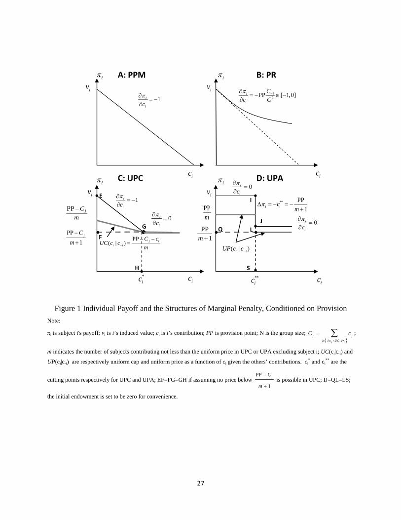
Figure 1 shows individual payoffs and the structures of marginal penalty for agent i under

different mechanisms, conditioned on provision. For PPM (Panel A), since excess contributions

10

will not be rebated and bring no additional benefits to subjects, every experimental dollar

contributed to the public good beyond PP will be wasted and thus the marginal penalty of over

contribution is -1. For PR (Panel B), the marginal penalty is (Marks and Croson,

1998), where 𝐶 = ∑ 𝑐𝑗𝑗 and 𝐶−𝑖 = ∑ 𝑐𝑗𝑗≠𝑖 . This is bounded between -1 and 0, and typically

greater than -1. Marks and Croson argue the lower marginal penalty will lead to higher

contributions under PR than PPM.

UPC has a different marginal penalty structure from PR and PPM, although the set of UPE is the

same. It can be discussed in two cases. First, if the ci being incremented is at or above UC(ci|c-i),

then any incremental contribution will not change the uniform price and will be fully rebated,

creating a marginal penalty of 0. Second, if ci< UC(ci|c-i), the marginal penalty is illustrated in

Figure 1 (Panel C). Here, there exists a cutting point, ci*, at which the marginal penalty changes

from -1 to 0. In Figure 1, the intercept of the grey solid line with the y-axis represents the

realized uniform price when ci=0. When approaching ci* from below, UC(ci|c-i) decreases and

the increased contribution is fully collected, leading to a marginal penalty of -1; when

approaching ci* from above, UC(ci|c-i) stays constant at ci

* and the marginal penalty is 0; at ci

=ci*, marginal penalty is not defined. Based on these expected marginal penalities (with

expectations taken over beliefs about c-i implied by various UPE) between -1 and 0, we would

expect higher aggregate contributions in UPC than in PPM, while UPC and PR might be

comparable.

The marginal penalty structure of UPA is similar to that of UPC, but with a critical difference. If

ci<UP(ci|c-i) (Figure 1, Panel D) where UP(ci|c-i) involves payments of PP/m by m other agents,

there exists a cutting point, ci**, at which i’s contribution is sufficient that it can be included in

payments of the next lowest uniform price, and the final payment by i jumps from 0 to the new

price, UP(ci**|c-i)= 𝑃𝑃

𝑚+1. At all other points, the marginal penalty is 0, even when the

contribution is lower than ci**. Thus, the marginal penalty of UPA is zero almost always, except

at the cutting point with a lump sum penalty. Given the broad range of values with no marginal

penalty, we conjecture higher contributions in UPA than the other mechanisms.

11

Note that the marginal penalty structures of UPC and UPA not only suggest differences in

aggregate contributions among mechanisms, but if agents with higher vis tend to make higher

contributions, they are also suggestive of how incentives may differ across the range of values.

Since the marginal penalties vary with contribution level, agents offering a constant share of

their vis will be treated differently in UPC and UPA: higher contributions may be seen from high

value people in UPC and UPA than in PPM and PR, because the marginal penalty for higher

contributions is lower. Following the same logic, we would also expect a higher contribution

level from low value people in UPA than in the other mechanisms, while the contribution level

from low value people in UPC could be higher or lower than that from PPM or PR.

4 Experimental Design and Procedures

To test the predictions of UPE and the effects of marginal penalty among the four mechanisms,

we designed a controlled laboratory experiment in which agents with heterogeneous values make

contributions toward an induced value public good. In addition to varying the mechanism,

treatments also varied PP to alter where in the range of values the provision outcome was likely

to be binding.

Table 1 shows the treatments presented in each session, with a treatment designated by the

mechanism abbreviation and PP. The first treatment is always PPM (10 rounds), which is used to

get subjects familiar with the baseline game. The following treatments (15 rounds each) apply

the other mechanisms and provision points in a partial Latin Square to control for order effects.

In each session, sixteen to twenty subjects were seated in private computer carrels in the

laboratory. At the start of each treatment, the experimenter read the instructions (see the

Appendices) aloud as subjects read along. Subjects were then given an initial budget of 14

experimental dollars to begin the treatment. Prior to each round, subjects were randomly

assigned to equally-sized groups (off-by-one if the number of subjects in a session was odd),4

4 The instructions indicated group size would be 5 to 12.

and assigned a vi. The private vis were drawn from an (unknown) distribution on the common-

knowledge range of 4 to 12, in dollar increments: four, five and six had probability of 3/15 each;

12

seven to twelve had probability of 1/15 each.5

Subjects then simultaneously choose a

contribution, ci∈[0,14] towards of the project. At the end of each round, subjects were informed

whether the project is provided, and their earnings, payment and rebates. At the end of a session,

earnings were totaled across all rounds.

The unknown PP for a group of N subjects was set at α • (6.8N), where 6.8 is the average vi and α a

treatment parameter. In Sessions 1 to 6, α was set at 0.6 of expected induced value for PPM, PR,

and UPC; UPA was reduced to α of 0.3 after pilots with nearly zero provision rate. In Sessions 7

to 12, we used α of 0.3, 0.6, and 0.9, as shown in Table 1. We denote the provision point

treatments as PP0.3, PP0.6, and PP0.9, respectively. For UPA, α of 0.36 was chosen based on

simulations that suggested a similar provision rate as the other mechanisms at α of 0.6.

Subjects were recruited from introductory economics classes and from an email list of students

interested in participating in experiments. A total of 226 subjects participated in the twelve

complete sessions, leading to an average group size of 9 (two groups in each round), and an

average payment of $32 for roughly 90 minutes. The software z-Tree (Fischbacher, 2007) is

used for the program.

5 Group Contribution Results

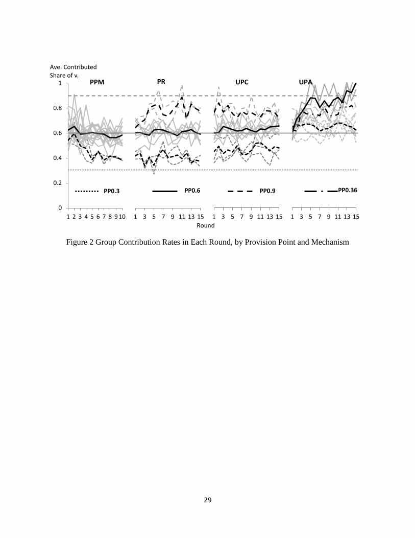
Figure 2 gives an overview of group contribution data in each round by provision point and

mechanism. Aggregate contributions are rescaled by session-round-specific aggregate induced

values in order to make them comparable across groups with different group sizes. Grey lines

represent group contributions from each session, and dark lines represent averages at each PP.

Figure 2 shows that, in each treatment, average aggregate contributions stabilize after roughly

five rounds. Across mechanisms, higher provision points lead to higher contributions: subjects

are tracking down the provision point and contributing in its neighborhood, even though group

members are reshuffled in each round. Comparing across mechanisms, UPA has considerably

5 This structure is chosen to mirror an underlying value distribution of interest to the funder, i.e., many people value the good a little, some value moderately and a few value it a lot.

13

higher contributions at each provision point level, and UPC looks to be slightly higher than PR

and PPM at PP0.3 and PP0.6.

The results below characterize statistically these observations, focusing on data from after the

first five periods of each treatment.

Result 1: Group contributions are not equal to the UPE predicted level of the provision point in

PPM, PR, and UPC. However, consistent with UPE, contributions are above the provision point

in UPA; and contributions in all mechanisms are higher when provision points are higher.

Figure 3 shows average group contributions at each PP for each mechanism, excluding the first 5

rounds of each treatment6

. The provision point axis represents α. The group contribution is the

average fraction of total induced value contributed.

First, group contributions in PPM, PR, and UPC are inconsistent with the specific UPE

prediction that, under complete information, contributions will exactly equal PP. Only for PR

with PP0.6 does a two-tailed t-test fail to reject the hypothesis that contributions are equal to the

provision point (p=0.903). At PP0.3, contribution rates are 40.9% (PPM; p<0.001), 40.2% (PR;

p<0.001), and 45.1% (UPC; p<0.001); at PP0.6, 58.1% (PPM; p=0.020) and 63.0% (UPC;

p<0.001); at PP0.9, 78.1% (PR; p<0.001) and 75.2% (UPC; p<0.001); all are significantly

different than the provision point. This contrasts with Marks and Croson (1998), who found

average group contributions under PPM and PR are not statistically distinguishable from PP, and

could be attributable to the heterogeneous values or unknown provision point in our experiment.

UPA contributions are consistent with the UPE prediction that they may exceed the provision

point. At PP0.3, the contribution rate is 64.8% (p<0.001), 77.7% at PP0.36 (p<0.001), and 87.9%

at PP0.6 (p<0.001). Because PP is only the lower bound of the UPA equilibrium set, these

results are not by themselves inconsistent with UPE strategies.

6 Conclusions are robust to excluding different numbers of initial rounds.

14

While the precise prediction of UPE does not hold, the comparative static prediction that

contribution rates increase with provision points does, though they are biased toward one half.

In PPM, PR, and UPC, group contributions increase from approximately 40% to 60% and 75%

when PP increases from 0.3 to 0.6 and 0.9; in UPA, they increase from 65% to 78% to 88% as

the PP increases from 0.3 to 0.36 to 0.6. By t-test, group contributions are signifincantly

different (at the 0.01 level or better) from each other for any pair of provision point levels within

each mechanism.

One important difference between UPA and the other mechanisms that could be driving

differences in contributions is in the provision rule that may require contributions above PP, and

may thus lower the provision rate. Result 2 compares provision rates across mechanisms.

Result 2: UPA has a significantly lower provision rate than the other mechanisms; UPC has a

significantly higher provision rate than PR and PPM at moderate provision points, but the

differences disappear at low or high provision points; PR and PPM have similar provision rates.

Figure 4 shows how average provision rates vary with PP among mechanisms. Given our

induced value distribution and chosen rates, provision was the efficient outcome for 100% of

groups at PP0.3, PP0.36 in all mechanisms; for 100% of groups at PP0.6 in all mechanisms but

UPA, which was 55.0%; and for 77.5% of PR groups and 85.0% of UPC groups at PP0.9.

Provision rates strongly decrease at higher provision points, a result consistent with Isaac et al.

(1989) and Suleiman and Rapoport (1992). The level and rate of decrease are significantly

different among mechanisms. Due to its constraints on the distribution of the contributions, UPA

has a dramatically lower provision rate at every PP than the other mechanisms. For PPM, PR

and UPC, however, we cannot reject the hypothesis of similar provision rates at PP0.3, where

provision is easy, and at PP0.9, where provision is very difficult. It is at PP0.6, where marginal

changes in contributions affect outcomes, that differences emerge among mechanisms: UPC has

a 60.7% provision rate, followed by PR at 48.3% (z-test p=0.045 different from UPC) and PPM

at 42.9% (p=0.377 below PR but p=0.003 below UPC). These differences parallel differences in

contribution rates, and thus may be key drivers of contribution dynamics, as subjects try to

15

contribute just enough to obtain regular provision as a group, but also minimize their individual

costs (cf. Issac et al.’s (1989) notion of cheap riding).

In order to understand the observed differences in contributions and provision rates beyond what

UPE predicts, we focus on the effect of marginal penalty to analyze individual and group data.

The first result finds a broad effect of marginal penalty, controlling for provision point and

provision rate.

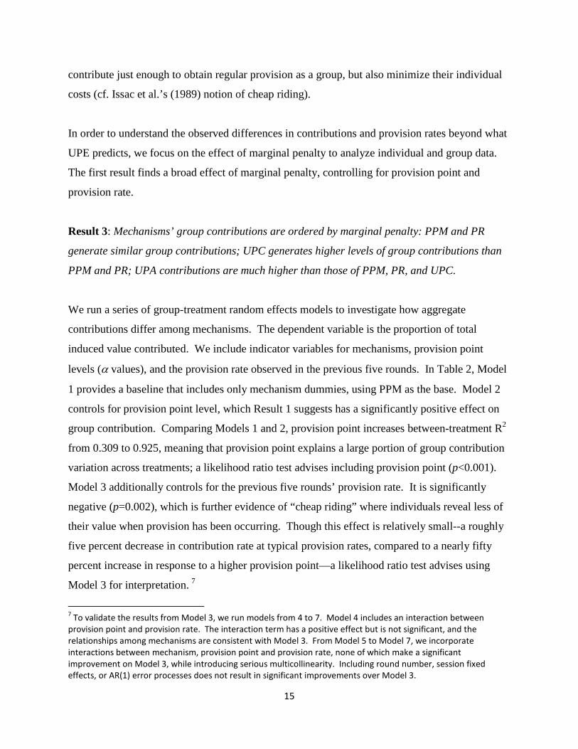
Result 3: Mechanisms’ group contributions are ordered by marginal penalty: PPM and PR

generate similar group contributions; UPC generates higher levels of group contributions than

PPM and PR; UPA contributions are much higher than those of PPM, PR, and UPC.

We run a series of group-treatment random effects models to investigate how aggregate

contributions differ among mechanisms. The dependent variable is the proportion of total

induced value contributed. We include indicator variables for mechanisms, provision point

levels (α values), and the provision rate observed in the previous five rounds. In Table 2, Model

1 provides a baseline that includes only mechanism dummies, using PPM as the base. Model 2

controls for provision point level, which Result 1 suggests has a significantly positive effect on

group contribution. Comparing Models 1 and 2, provision point increases between-treatment R2

from 0.309 to 0.925, meaning that provision point explains a large portion of group contribution

variation across treatments; a likelihood ratio test advises including provision point (p<0.001).

Model 3 additionally controls for the previous five rounds’ provision rate. It is significantly

negative (p=0.002), which is further evidence of “cheap riding” where individuals reveal less of

their value when provision has been occurring. Though this effect is relatively small--a roughly

five percent decrease in contribution rate at typical provision rates, compared to a nearly fifty

percent increase in response to a higher provision point—a likelihood ratio test advises using

Model 3 for interpretation. 7

7 To validate the results from Model 3, we run models from 4 to 7. Model 4 includes an interaction between provision point and provision rate. The interaction term has a positive effect but is not significant, and the relationships among mechanisms are consistent with Model 3. From Model 5 to Model 7, we incorporate interactions between mechanism, provision point and provision rate, none of which make a significant improvement on Model 3, while introducing serious multicollinearity. Including round number, session fixed effects, or AR(1) error processes does not result in significant improvements over Model 3.

16

Model 3 reflects an ordering of contribution rates generated by each mechanism that is broadly

consistent with higher contributions occurring where the expected marginal penalty is lower,

especially for the marginal penalty structures of our new mechanisms. UPA—with an almost-

everywhere zero marginal penalty that expands the single-element equilibrium outcome set (the

provision point) to a continuum range of contributions where PP is only the lower bound—is

significantly higher than PPM (likelihood ratio p<0.001), PR (p<0.001) and UPC (p<0.001).

Similarly, the lower expected marginal penalty from UPC leads to significantly higher aggregate

contributions than PPM (p=0.006) and PR (p=0.084). Increasing contributions for a higher

probability of provision will not result in losing money in a broad contribution range in these

mechanisms. However, controlling for other covariates, we cannot reject the hypothesis that PR

and PPM generate the same aggregate contributions, consistent with Marks and Croson (1998).

To further test the marginal penalty story, we examine individual level contributions at different

induced values, where marginal penalty makes different predictions across mechanisms.

6 Individual Contribution Results

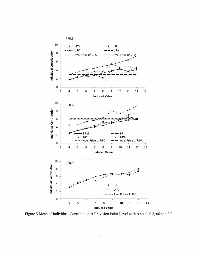
Figure 5 shows average individual contributions at each induced value across provision points

and mechanisms. Average observed uniform prices from UPA and UPC are also shown to

calibrate how being close to the kink in the marginal penalty function in those mechanisms

affects contributions. Looking across values, the amount contributed is increasing in induced

value in all mechanisms and at all provision points. As with aggregate contributions, UPA

stands out as generating much higher contributions, and UPC has generally slightly higher

contributions at all value levels.

To investigate statistically how individual contribution varies with induced value, provision point,

and mechanism, we run a series of subject-treatment random effects tobit models of dollar

amount contributed, incorporating all data except the first five rounds and including UPA at

PP0.36 (not shown in Figure 5). Table 3 shows the results, using PPM as an excluded base

mechanism. In the experiments, subjects are asked to make an offer from 0 up to 14

experimental dollars.

17

In Table 3, Model 1 is a baseline model which estimates mechanism-specific intercepts with

mechanism dummies; intercept variation with a PP term; variation in slope captured by induced

value; and provision point based variation in slope with an interaction of PP and value. Various

interaction terms among mechanisms, provision point, and induced value are added in Models 2

to 5, of which Model 3 is the most reliable. Models 2, 4, and 5 either involve many insignificant

interaction terms or suffer from serious multicolinearity. Model 6 has significantly lower log-

likelihood, but loses the significance of PP due to colinearity. Thus, we interpret Model 3, as it

has similar signs and significance, and is straightforward to explain. Three results are supported

by the regressions.

Result 4: In all mechanisms, contributions increases with higher induced values.

Value alone is large and statistically significantly positive (p<0.001), and there are no offsetting

negative coefficients on the individual mechanisms. This result provides strong statistical

evidence of a positive relationship between individual contribution and induced value, which has

not been widely documented across provision point mechanisms, though Rondeau et al. (2005)

and Spencer et al (2009) find similar effects in one-shot PR games. For PPM, the result is

consistent with related theoretical predictions (Alboth et al., 2001; Laussel and Palfrey, 2003;

Barbieri and Malueg, 2008).

Result 5: As provision point increases, the intercept and the slope of the contribution functions

also increase.

The significantly positive (p<0.001) coefficient on PP reflects that contributions increase when

the provision point does, and the significantly positive interaction with value (p<0.001) indicates

people with higher values contribute proportionately more as PP increases. The effect here is

rather large, as an increase from α=0.3 to α=0.6 in PPM increases the contribution by 1.459

(=2.775*(0.6-0.3) + 0.209*(0.6-0.3)*10) dollars at a value of 10. Combining the positive effects

on both the intercept and the slope, this result is consistent with the result that aggregate

contribution increases with PP.

18

Result 6: UPA generates higher contributions across values, and proportionately larger

contributions at higher values; UPC has a significantly higher slope than PPM and PR.

Based on Model 3, the intercept and the slope of UPA’s contribution function are significantly

higher than those for PPM (intercept p=0.001; slope p<0.001) and PR (intercept p<0.001; slope

p<0.001). UPA has a significantly higher intercept (p<0.001) and a higher (not significantly, p =

0.220) slope than UPC. Combined, these results indicate that UPA generates higher

contributions throughout the value range. This effect is relatively large, at a value of 10 with

α=0.3, the predicted UPA contribution is $2.375 (=0.859+0.148*10) higher than PPM, $2.194

(=0.895+0.294+(0.148-0.0475)*10) higher than PR and $1.762 (=0.895+0.587+(0.148-0.12)*10)

higher than UPC.

UPC has a slightly lower intercept than PPM (p = 0.018) and is not distinct from PR (p = 0.249).

Its contribution function has a significantly higher slope throughout the range of induced values,

which implies UPC elicits higher contributions from higher valued people than do PPM and PR.

PR and PPM look similar. Although PR has a borderline significantly (p=0.051) higher slope

than PPM, it has a small, negative intercept (-0.294) that suggests that the intersection of PPM

and PR’s contribution functions is around a low-end induced value of 6 (0.294/0.0475≈6.2), and

that PR generates an economically meaningful increase in contributions only among those with

the highest induced values.

Organizing these contribution function results according to the marginal penalty benchmark

requires further decomposing the data, because the expected marginal penalty varies throughout

the value range. Further, the different values at which the contribution functions in Figure 5

intersect the average uniform prices for UPA and UPC suggest that the marginal penalty at a

given value may vary with mechanism. To capture this, we compare mechanisms within each of

three ranges of induced value. In the low range, even contributions of a high proportion of

induced value have small effect on the provision likelihood; this is also the range where UPA

and UPC are distinct. In the high range, contributions of a relatively small portion of value

19

considerably affect the likelihood of provision; this is the range where PPM and PR are most

different from the uniform price mechanisms. In the medium range, contributions typically fall

near the observed uniform prices in UPA and UPC. We use differences in contribution behavior

within these value ranges to explore how differences among mechanisms are related to their

marginal penalty structures.

We use two conventions to define value levels. First, we divide the value range evenly into three

levels: 4-5-6 as a low level, 7-8-9 as medium, and 10-11-12 as high. This partition is neutral to

any marginal penalty structure and especially suitable for PPM and PR, since their marginal

penalties are continuous in contribution. Second, we group values based upon the expected

marginal penalties of people with those values, which is appropriate for the discrete marginal

penalty structure of UPA and UPC. As shown in Figure 1, the marginal penalty in UPC and

UPA changes significantly around the uniform price, which naturally differentiates induced

values based on the relationship between value and contribution. We identify who expects to

make contributions in each range of marginal penalty by calculating the mean price8

for UPC

and UPA, and consider contributions within one standard deviation of the mean as “close” to the

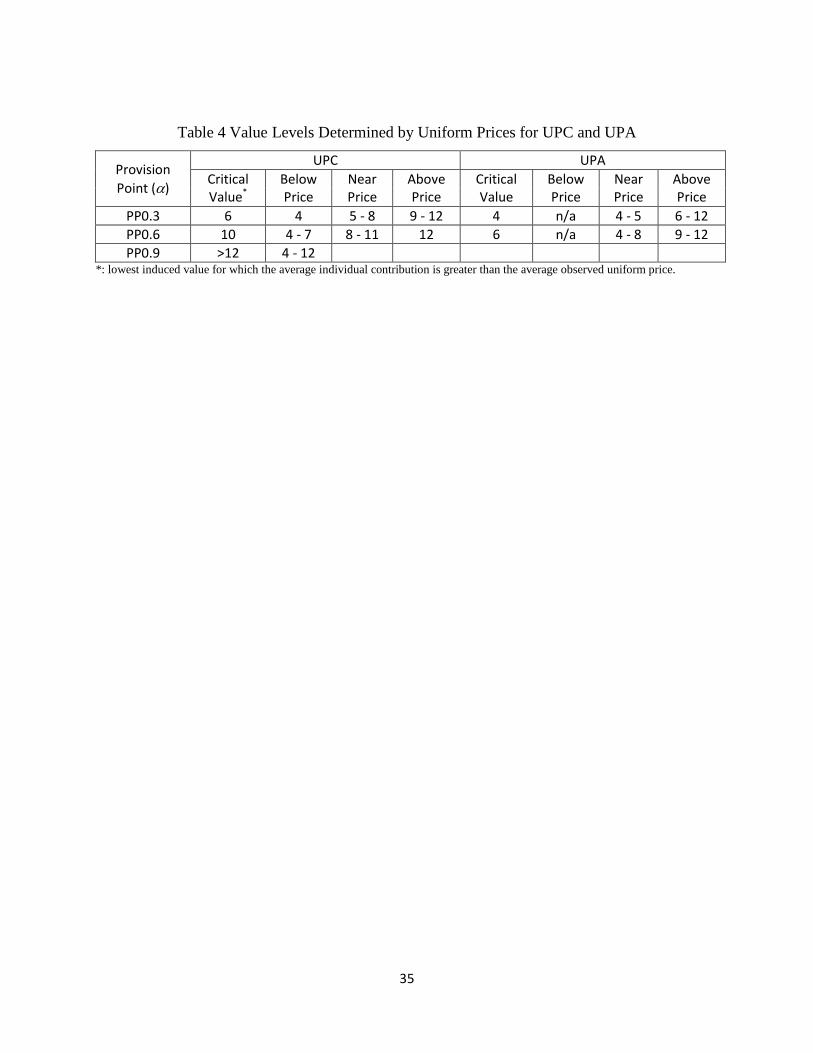
uniform price. Then, for each mechanism, we look at the induced values for which the average

contributions are clearly below the uniform price, clearly above it, or likely to be near the

observed uniform price. The resulting induced value levels for UPA and UPC at each provision

point are shown in Table 4.

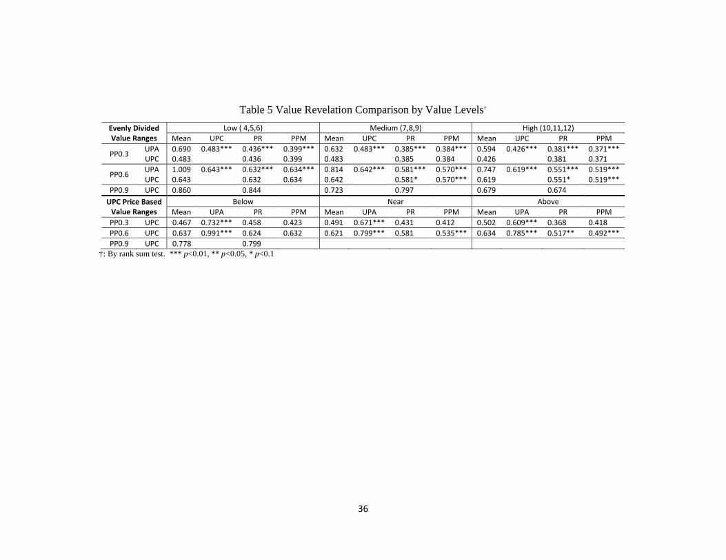
To pool contributions at different values within each value level, we use the ratio of contribution

to value to measure value revelation. Then we pairwise compare value revelations of different

mechanisms within each value level. Table 5 shows the value revelation comparisons based on

evenly divided and UPC-price-based value levels. For example, at the low value level of PP0.3,

the average value revelations in UPA and PR are respectively 0.690 and 0.436, which are

different at the 0.01 significance level by a Wilcoxon rank sum test; the next row compares UPC

to the other mechanisms.

8 Ideally, the uniform prices for UPA and UPC can be calculated ex ante based on contribution functions in equilibrium, and the value levels for each mechanism can be determined accordingly. However, the contribution functions have not been solved yet, so we use this feasible empirical benchmark.

20

Comparing mechanisms within each level provides three key results consistent with agents’

responding to differences in marginal penalty in making their contribution choices.

Result 7: Consistent with the marginal penalty effect, value revelation is significantly higher in

UPA than the other mechanisms, throughout the value range.

Regardless of the how value levels are determined,9

UPA generates significantly (at 0.01 level)

higher contributions from the other three mechanisms across all three value levels, which is

consistent with Result 6 and the pattern shown in Figure 5. The marginal penalty argument

explains well here: by having zero marginal penalty across most of the value range, UPA

generates significantly higher contributions over the value range. Importantly, this is true even

in the range of observed uniform prices (near), as this is where there is a risk of a discrete jump

in penalty from an incrementally higher contribution.

Together, Results 6 and 7 add that UPA generates significantly higher contributions not only in

aggregate, but also at each induced value level. The performance of UPC relative to the other

mechanisms varies by value level and depends on the provision point, and is reported in two

results.

Result 8: UPC generates comparable value revelation with PR and PPM at all value levels

when the provision point is low; UPC and PR are comparable at all value levels at higher

provision points.

Table 5 indicates UPC is not significantly different from PPM and PR when at PP0.3, and

additionally PR at PP0.9, at any value level. Since, at high induced values, the marginal penalty

of UPC is zero compared to positive and close to one for PPM and PR, this is evidence against

the marginal penalty model. However, combined with the next result, it shows that there is an

important additional condition for the marginal penalty effect to be observed: salience.

9 Table 5 only shows the evenly divided value levels for UPA; value levels based on the UPA uniform price lead to the same significance levels.

21

Result 9: At moderate provision points, UPC generates significantly higher value revelation

than PPM at near- and above-price values; UPC generates significantly higher value revelation

than PR at above-price value levels.

Understanding how UPC is different than PR and PPM requires focusing on value levels defined

based on proximity to observed UPC uniform prices, in the lower section of Table 5. The

marginal penalty is the same (-1) for UPC and PPM at below-price values and, as expected,

value revelation from UPC and PPM is not significantly different at PP0.6 (0.637 vs. 0.632,

p=0.140). At above-price values, marginal penalties are different between UPC (0) and PPM (-

1), and the PP0.6 value revelations of UPC and PPM are accordingly significantly (at 0.01 level)

different.

UPC generates significantly higher contributions than PR in PP0.6 treatment at above-price

values (p=0.030), but not at near- (p=0.184) and below- (p=0.383) price value levels. At high

levels, marginal penalties are different between UPC (0) and PR (smaller than, but generally

close to, -1 in PP0.6), so the significant difference is consistent with agents responding to

marginal penalty. At the below-price level, UPC’s marginal penalty is -1, and PR’s remains

close to -1, so comparable contributions are consistent with the marginal penalty effect; the

insignificant difference in the neighborhood of the UPC uniform price is similarly explained.

Interpreting Results 8 and 9 jointly, contributions vary across mechanisms consistent with

marginal penalty, but only when there is sufficient incentive for agents to consider their

contributions carefully. At PP0.9, provision is difficult in all mechanisms, and thus one person’s

incremental contribution is very unlikely to affect the probability of provision and thus payoffs;

at PP0.3, provision is easy, occurring in nearly all PR, PPM and UPC rounds, typically with

aggregate contributions far above PP, and thus one person’s incremental contribution is unlikely

to affect payoffs by an economically meaningful amount. In both these cases, small changes in

contribution do not generate large enough changes in payoffs to lead subjects to a strategic

response that would allow us to detect differences in the incentives provided by the different

22

mechanisms.10

However, when incremental contribution changes are empirically sufficiently

likely to affect provision, mostly at PP0.6, subjects are considering their contribution decisions

more carefully. In these pivotal value ranges, differences among mechanisms are observed, and

the observed differences reflect subjects’ responding to differences in marginal penalty.

7 Conclusions

This paper introduces two new mechanisms for threshold public goods, based on uniform price

auctions: the uniform price auction mechanism (UPA) and the uniform price cap mechanism

(UPC). It seeks to establish whether they generate higher levels of contributions than the widely

studied provision point mechanism without a rebate (PPM), and with a contribution-proportional

rebate (PR). We first characterize these four mechanisms using the concepts of undominated

perfect equilibrium (UPE) and the marginal payment penalty associated with over-contribution.

Then we run experiments characterized by heterogeneous values, repetition, and varying

provision points to compare the mechanisms’ performance in terms of group contribution,

provision rate, and individual contribution across the range of induced values.

We have two observations about group contributions from the experiments: 1) after an

adjustment period, aggregate contributions are mainly determined by--but generally not equal

to—the provision point; 2) different mechanisms lead to significantly different levels of group

contributions. The first observation is associated with the provision point representing the

aggregate equilibrium outcome of UPE. Whether it is known or not, the existence of a provision

point induces the group contribution to converge toward the minimum level of contribution that

allows subjects to secure the added benefit of the public good. However, strategic uncertainty

and heterogeneous values make it difficult to coordinate on a single distribution of the costs so

that the group contribution is exactly equal to provision point.

The most prominent feature of the second observation is that UPA group contributions are

significantly—statistically and economically—much higher than group contributions of the other 10 This is a property of the mechanisms at particular parameter values, rather than a flaw in salience of the experiment. Similar effects are seen in other institutions, such as measuring the values of extramarginal buyers in second price auctions.

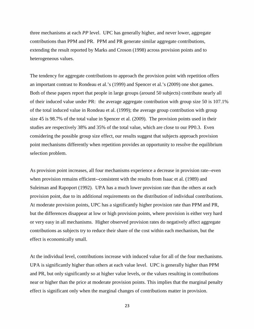
23

three mechanisms at each PP level. UPC has generally higher, and never lower, aggregate

contributions than PPM and PR. PPM and PR generate similar aggregate contributions,

extending the result reported by Marks and Croson (1998) across provision points and to

heterogeneous values.

The tendency for aggregate contributions to approach the provision point with repetition offers

an important contrast to Rondeau et al.’s (1999) and Spencer et al.’s (2009) one shot games.

Both of these papers report that people in large groups (around 50 subjects) contribute nearly all

of their induced value under PR: the average aggregate contribution with group size 50 is 107.1%

of the total induced value in Rondeau et al. (1999); the average group contribution with group

size 45 is 98.7% of the total value in Spencer et al. (2009). The provision points used in their

studies are respectively 38% and 35% of the total value, which are close to our PP0.3. Even

considering the possible group size effect, our results suggest that subjects approach provision

point mechanisms differently when repetition provides an opportunity to resolve the equilibrium

selection problem.

As provision point increases, all four mechanisms experience a decrease in provision rate--even

when provision remains efficient--consistent with the results from Isaac et al. (1989) and

Suleiman and Rapoport (1992). UPA has a much lower provision rate than the others at each

provision point, due to its additional requirements on the distribution of individual contributions.

At moderate provision points, UPC has a significantly higher provision rate than PPM and PR,

but the differences disappear at low or high provision points, where provision is either very hard

or very easy in all mechanisms. Higher observed provision rates do negatively affect aggregate

contributions as subjects try to reduce their share of the cost within each mechanism, but the

effect is economically small.

At the individual level, contributions increase with induced value for all of the four mechanisms.

UPA is significantly higher than others at each value level. UPC is generally higher than PPM

and PR, but only significantly so at higher value levels, or the values resulting in contributions

near or higher than the price at moderate provision points. This implies that the marginal penalty

effect is significant only when the marginal changes of contributions matter in provision.

24

The difference between UPA and the other three mechanisms is fundamental in the sense that, in

equilibrium, UPA generally generates higher group contributions than the others, and hence

significantly higher group and individual contributions at all provision points and value levels

are observed in UPA. Group contributions in UPC exceed PPM and PR by less than those for

UPA because the UPE concept for UPA supports as equilibria strategies leading to aggregate

contributions above PP; the provision point is only a lower bound for UPA, while it is the entire

set for the other mechanisms. Among the mechanisms with a common set of UPE, UPC attracts

higher contributions because middle and higher value people can tender larger contributions,

knowing marginal increases will be rebated in full unless they are critical to provision. That

variation is so well explained by differences in equilibrium and marginal penalty incentive

properties suggests that the different notions of distributional fairness that motivated the uniform

price mechanisms are not primary determinants of success.

The novel UPA and UPC mechanisms do improve upon existing budget-balancing mechanisms

in value revelation and provision of a threshold public good. If valuation is the goal, UPA is the

best choice among the four mechanisms, as it elicits agents’ values most accurately. If actually

providing the public good is the major concern, UPC represents a meaningful improvement over

the well studied PPM and PR. This is especially true if the group being targeted for provision

has a relatively large proportion of high value people, in which case the zero or low marginal

penalty in the uniform price mechanisms allows them to make larger contributions, more fully

revealing their values and increasing prospects for provision.

25

References

Alboth, D., Lerner, A. and Shalev, J. (2001), Profit maximizing in auctions of public goods,

Journalof Public Economic Theory, 3 (4): 501-525.

Bagnoli, M. and Lipman, B. L. (1989), Provision of Public-Goods - Fully Implementing the Core

through Private Contributions, Review of Economic Studies, 56 (4): 583-601.

Bagnoli, M. and McKee, M. (1991), Voluntary Contribution Games - Efficient Private Provision

of Public-Goods, Economic Inquiry, 29 (2): 351-366.

Bagnoli, M., Bendavid, S. and McKee, M. (1992), Voluntary Provision of Public-Goods - the

Multiple Unit Case, Journal of Public Economics, 47 (1): 85-106.

Barbieri, S. and Malueg, D. A. (2008), Private Provision of a Discrete Public Good: Efficient

Equilibria in the Private-information Contribution Game, Economic Theory, 37 (1): 51-80.

Barbieri, S. and Malueg, D. A. (2010a), Threshold uncertainty in the private-information

subscription game, Journal of Public Economics, 94 (11-12): 848-861.

Barbieri, S. and Malueg, D. A. (2010b), Profit-Maximizing Sale of a Discrete Public Good via

the Subscription Game in Private-Information Environments, B E Journal of Theoretical

Economics, 10 (1): Article 5.

Cason, T. N. and Gangadharan, L. (2004), Auction design for voluntary conservation programs,

American Journal of Agricultural Economics, 86 (5): 1211-1217.

Cason, T. N. and Gangadharan, L. (2005), A laboratory comparison of uniform and

discriminative price auctions for reducing non-point source pollution, Land Economics,

81 (1): 51-70.

Chen, Y. (2008). Incentive-compatible Mechanisms for Pure Public Goods: A Survey of

Experimental Research. In: and Charles, R.P. and. Smith, V.L., Editors, 2008. Handbook

of Experimental Economics Results. North-Holland, Amsterdam, The Netherlands,

Volume 1: 625-643.

Davis, D. and Holt, C. (1993), Experimental Economics, Princeton University Press, Princeton,

NJ, p.317 – 379.

Evans, M. F., Vossler, C. A. and Flores, N. E. (2009), Hybrid allocation mechanisms for publicly

provided goods, Journal of Public Economics, 93 (1-2): 311-325.

Fischbacher, U. (2007), z-Tree: Zurich Toolbox for Ready-made Economic Experiments,

26

Experimental Economics, 10 (2): 171-178.

Gailmard, S. and Palfrey, T. R. (2005), An experimental comparison of collective choice

procedures for excludable public goods, Journal of Public Economics, 89 (8): 1361-1398.

Isaac, R. M., Schmidtz, D. and Walker, J. M. (1989), The assurance problem in a laboratory

market, Public Choice, 62 (3): 217-236.

Jack, B. K., Leimona, B. and Ferraro, P. J. (2009), A revealed preference approach to estimating

supply curves for ecosystem services: use of auctions to set payments for soil erosion

control in Indonesia, Conservation Biology, 23 (2): 359-367.

Laussel, D. and Palfrey, T. R. (2003), Efficient Equilibria in the Voluntary Contributions

Mechanism with Private Information, Journal of Public Economic Theory, 5 (3): 449-478.

Ledyard, J.O., (1995). Public goods: a survey of experimental research. In: Kagel, J.H. and Roth,

A.E., Editors, 1995. The Handbook of Experimental Economics, Princeton University Press,

Princeton, New Jersey, pp. 111–194.

Marks, M. and Croson, R. (1998), Alternative rebate rules in the provision of a threshold public

good: An experimental investigation, Journal of Public Economics, 67 (2): 195-220.

McBride, M. (2006), Discrete public goods under threshold uncertainty, Journal of Public

Economics, 90 (6-7): 1181-1199.

Menezes, F. M., Monteiro, P. K. and Temimi, A. (2001), Private provision of discrete public

goods with incomplete information, Journal of Mathematical Economics, 35 (4): 493-514.

Nitzan, S. and Romano, R. E. (1990), Private Provision of a Discrete Public Good with

Uncertain Cost, Journal of Public Economics, 42 (3): 357-370.

Rondeau, D., Poe, G. L. and Schulze, W. D. (2005), VCM or PPM? A comparison of the

performance of two voluntary public goods mechanisms, Journal of Public Economics, 89

(8): 1581-1592.

Rondeau, D., Schulze, W. D. and Poe, G. L. (1999), Voluntary revelation of the demand for

public goods using a provision point mechanism, Journal of Public Economics, 72 (3): 455-

470.

Spencer, M. A., Swallow, S. K., Shogren, J. F. and List, J. A. (2009), Rebate rules in threshold

public good provision, Journal of Public Economics, 93 (5-6): 798-806.

Suleiman, R. and Rapoport, A. (1992), Provision of Step-level Public Goods with Continuous

Contribution, Journal of Behavioral Decision Making, 5 (2): 133-153.

27

Figure 1 Individual Payoff and the Structures of Marginal Penalty, Conditioned on Provision

Note:

πi is subject i's payoff; vi is i’s induced value; ci is i’s contribution; PP is provision point; N is the group size; { }: ,∈ < ≠

= ∑j j

jj j c UC j i

C c ;

m indicates the number of subjects contributing not less than the uniform price in UPC or UPA excluding subject i; UC(ci|c-i) and

UP(ci|c-i) are respectively uniform cap and uniform price as a function of ci given the others’ contributions. ci* and ci

** are the

cutting points respectively for UPC and UPA; EF=FG=GH if assuming no price below PP

1

−

+

jC

m is possible in UPC; IJ=QL=LS;

the initial endowment is set to be zero for convenience.

iπ iπ

iπ ic ic

ic ic

iv

iπ

iv

iv

iv

PPm

PP1m +

PP − jCm

PP1

−+

jCm PP

( | )−

− −= j i

i i

C cUC c c

m

1i

icπ∂

= −∂

1i

icπ∂

= −∂

2PP [ 1,0]i i

i

Cc Cπ −∂

= − ∈ −∂

0i

icπ∂

=∂

0i

icπ∂

=∂

0i

icπ∂

=∂

** PP1i ic

mπ∆ = − = −

+

**ic

A: PPM

C: UPC

B: PR

D: UPA

*ic

( | )i iUP c c−

E

F

G

Q

I

J

L

H

S

• • •

28

Table 1 Treatment Arrangement of Experimental Sessions

Treatment Order 1st (10 rounds) 2nd (15 rounds) 3rd (15 rounds) 4th (15 rounds) Session 1 PPM (0.6) PR (0.6) UPC (0.6)

Session 2 PPM (0.6) PR (0.6) UPA (0.3) Session 3 PPM (0.6) UPC (0.6) PR (0.6) Session 4 PPM (0.6) UPC (0.6) UPA (0.3) Session 5 PPM (0.6) UPA (0.3) PR (0.6) Session 6 PPM (0.6) UPA (0.3) UPC (0.6) Session 7 PPM (0.3) PR (0.3) UPC (0.3)

Session 8 PPM (0.3) UPC (0.3) PR (0.3) PR (0.6) Session 9 PPM (0.6) UPC (0.6) UPA (0.6) UPA (0.3) Session 10 PPM (0.6) UPA (0.6) UPC (0.6) UPC (0.3) Session 11 PPM (0.6) UPA (0.36) UPC (0.9) PR (0.9) Session 12 PPM (0.6) PR (0.9) UPA (0.36) UPC (0.9) Session A1 PPM (0.6) UPC (0.6) Session A2 PPM (0.6) UPA (0.3) Session A3 PPM (0.6) UPA (0.6) Session A4 PPM (0.3) PR (0.6)

Note: the number in the parentheses is the provision point in terms of the percentage of expected total induced value. Sessions

A1-4 had software problems, but we use data collected prior to the program crash.

29

Figure 2 Group Contribution Rates in Each Round, by Provision Point and Mechanism

0

0.2

0.4

0.6

0.8

1

1 2 3 4 5 6 7 8 9 10

PP0.3

1 3 5 7 9 11 13 15

PP0.6

1 3 5 7 9 11 13 15

PP0.9

1 3 5 7 9 11 13 15

PP0.36

UPA PR PPM UPC

Round

Ave. Contributed Share of vi

30

Figure 3 Average Group Contribution Rate at Each Provision Point

0

0.2

0.4

0.6

0.8

1

0.2 0.4 0.6 0.8 1

Gro

up C

ontr

ibut

ion

Rate

Provision Point

PPM

PR

UPC

UPA

31

Figure 4 Average Provision Rate at Each Provision Point

0

0.2

0.4

0.6

0.8

1

0.2 0.4 0.6 0.8 1

Prov

isio

n Ra

te

Provision Point

PPM

PR

UPC

UPA

32

Table 2 Random Effects Models of Group Contribution Rate Group Contribution Rate (1) (2) (3)

PR 0.0365 0.0141 0.0138

(0.0398) (0.0154) (0.0165)

UPC 0.0464 0.0389*** 0.0435***

(0.0377) (0.0147) (0.0158)

UPA 0.175*** 0.276*** 0.258***

(0.0387) (0.0161) (0.0182)

PP

0.596*** 0.485***

(0.0346) (0.0517)

Provision Rate

-0.0890*** Based on previous 5 rounds†

(0.0288)

Constant 0.560*** 0.224*** 0.337***

(0.0249) (0.0220) (0.0434)

log-likelihood 512.9 560.5 565.3 Chi-Square 17.97*** 113.1*** 122.7*** R2_within treatment 0.000 0.00349 0.0483 R2_between treatment 0.309 0.925 0.908 R2_overall 0.249 0.745 0.739 Obs: 410 No. of Group: 49 Tbar = 7.538 g_max = 10 g_ave = 8.367 g_min = 5

Standard errors in parentheses; *** p<0.01, ** p<0.05, * p<0.1 †: Number of times provided by the two groups in each session in the previous five rounds, divided by 10

33

Figure 5 Mean of Individual Contribution at Provision Point Level with α set to 0.3, 06 and 0.9

0

2

4

6

8

10

3 4 5 6 7 8 9 10 11 12 13

Indi

vidu

al C

ontr

ibut

ion

Induced Value

PPM PR UPC UPA Ave. Price of UPC Ave. Price of UPA

0

2

4

6

8

10

3 4 5 6 7 8 9 10 11 12 13

Indi

vidu

al C

ontr

ibut

ion

Induced Value

PPM PR UPC UPA Ave. Price of UPC Ave. Price of UPA

0

2

4

6

8

10

3 4 5 6 7 8 9 10 11 12 13

Indi

vidu

al C

ontr

ibut

ion

Induced Value

PR

UPC

Ave. Price of UPC

PP0.6

PP0.9

PP0.3

34

Table 3 Random Effects Tobit Models of Individual Contribution

Contribution (1) (2) (3) (4) (5) (6) PR 0.0320 -0.187 -0.294 -0.293 0.311 -0.285

(0.196) (0.859) (0.257) (0.257) (1.215) (0.258)

UPC 0.237 0.577 -0.587** -0.587** -0.0793 -0.480*

(0.188) (0.828) (0.249) (0.249) (1.183) (0.250)

UPA 1.908*** 1.499* 0.895*** 0.904*** 0.925 0.621**

(0.209) (0.848) (0.272) (0.273) (1.198) (0.278)

PP 3.436*** 3.384*** 2.775*** 2.813*** 3.485* 0.861

(0.549) (1.265) (0.571) (0.575) (1.828) (0.657)

PR*PP

0.371

-1.049

(1.464)

(2.078)

UPC*PP

-0.589

-0.894

(1.429)

(2.042)

UPA*PP

1.034

0.253

(1.700)

(2.320)

Value 0.450*** 0.450*** 0.313*** 0.348*** 0.378*** 0.186***

(0.0246) (0.0246) (0.0336) (0.0801) (0.111) (0.0553)

Value*PP 0.115*** 0.115*** 0.209*** 0.147 0.0942 0.329***

(0.0439) (0.0439) (0.0495) (0.138) (0.194) (0.0656)

PR*Value

0.0475* -0.0328 -0.0740 0.0466*

(0.0243) (0.0877) (0.123) (0.0241)

UPC*Value

0.120*** 0.128 0.0917 0.112***

(0.0237) (0.0857) (0.121) (0.0236)

UPA*Value

0.148*** 0.0937 0.0809 0.164***

(0.0255) (0.0878) (0.122) (0.0262)

PR*Value*PP

0.138 0.210

(0.148) (0.211)

UPC*Value*PP

-0.0136 0.0505

(0.145) (0.209)

UPA*Value*PP

0.112 0.120

(0.165) (0.228)

Provision Rate†

-1.604***

(0.264)

Provision Rate

0.104*** *Value

(0.0354)

Constant -1.672*** -1.643** -0.725** -0.749** -1.128 1.255**

(0.332) (0.720) (0.367) (0.370) (1.047) (0.494)

log-likelihood -15575 -15574 -15552 -15551 -15550 -15516 Chi-Square 4229*** 4231*** 4302*** 4306*** 4307*** 4229*** R2_within 0.387 0.387 0.390 0.391 0.391 0.399 R2_between 0.129 0.131 0.129 0.131 0.132 0.107 R2_overall 0.254 0.255 0.256 0.257 0.258 0.249 Observations=7705 Number of group=922 g_max=10 g_avg=8.357 g_min=5 Standard errors in parentheses; *** p<0.01, ** p<0.05, * p<0.1

†: Provision rate from previous 4 rounds. Sum up times of provision of the groups the individual is in from previous 4 rounds and divide it by 4. Other round numbers are also tested, while four results in the largest log-likelihood.

35

Table 4 Value Levels Determined by Uniform Prices for UPC and UPA

Provision Point (α)

UPC UPA Critical Value*

Below Price

Near Price

Above Price

Critical Value

Below Price

Near Price

Above Price

PP0.3 6 4 5 - 8 9 - 12 4 n/a 4 - 5 6 - 12 PP0.6 10 4 - 7 8 - 11 12 6 n/a 4 - 8 9 - 12 PP0.9 >12 4 - 12

*: lowest induced value for which the average individual contribution is greater than the average observed uniform price.

36

Table 5 Value Revelation Comparison by Value Levels† Evenly Divided Value Ranges

Low ( 4,5,6) Medium (7,8,9) High (10,11,12) Mean UPC PR PPM Mean UPC PR PPM Mean UPC PR PPM

PP0.3 UPA 0.690 0.483*** 0.436*** 0.399*** 0.632 0.483*** 0.385*** 0.384*** 0.594 0.426*** 0.381*** 0.371*** UPC 0.483

0.436 0.399 0.483

0.385 0.384 0.426

0.381 0.371

PP0.6 UPA 1.009 0.643*** 0.632*** 0.634*** 0.814 0.642*** 0.581*** 0.570*** 0.747 0.619*** 0.551*** 0.519*** UPC 0.643

0.632 0.634 0.642

0.581* 0.570*** 0.619

0.551* 0.519***

PP0.9 UPC 0.860

0.844

0.723

0.797

0.679

0.674

UPC Price Based Value Ranges

Below Near Above Mean UPA PR PPM Mean UPA PR PPM Mean UPA PR PPM

PP0.3 UPC 0.467 0.732*** 0.458 0.423 0.491 0.671*** 0.431 0.412 0.502 0.609*** 0.368 0.418 PP0.6 UPC 0.637 0.991*** 0.624 0.632 0.621 0.799*** 0.581 0.535*** 0.634 0.785*** 0.517** 0.492*** PP0.9 UPC 0.778

0.799

†: By rank sum test. *** p<0.01, ** p<0.05, * p<0.1

37

Appendices

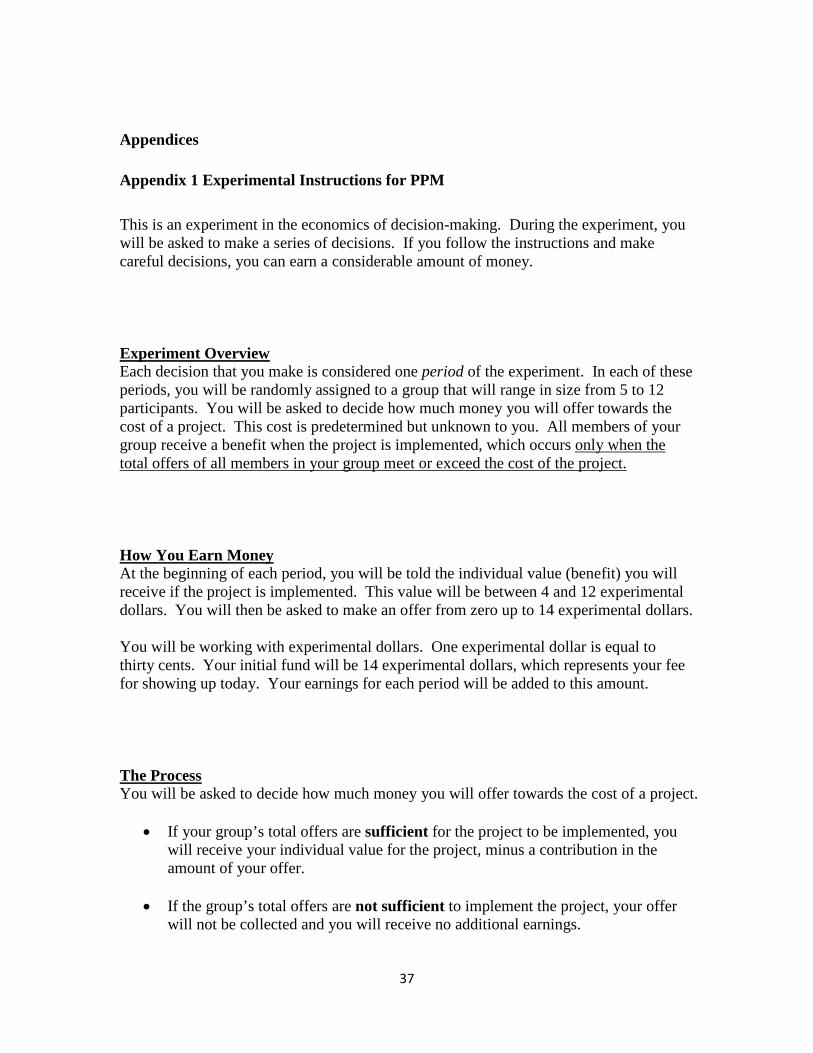
Appendix 1 Experimental Instructions for PPM

This is an experiment in the economics of decision-making. During the experiment, you will be asked to make a series of decisions. If you follow the instructions and make careful decisions, you can earn a considerable amount of money.

Each decision that you make is considered one period of the experiment. In each of these periods, you will be randomly assigned to a group that will range in size from 5 to 12 participants. You will be asked to decide how much money you will offer towards the cost of a project. This cost is predetermined but unknown to you. All members of your group receive a benefit when the project is implemented, which occurs

Experiment Overview

only when the total offers of all members in your group meet or exceed the cost of the project.

At the beginning of each period, you will be told the individual value (benefit) you will receive if the project is implemented. This value will be between 4 and 12 experimental dollars. You will then be asked to make an offer from zero up to 14 experimental dollars.

How You Earn Money

You will be working with experimental dollars. One experimental dollar is equal to thirty cents. Your initial fund will be 14 experimental dollars, which represents your fee for showing up today. Your earnings for each period will be added to this amount.

You will be asked to decide how much money you will offer towards the cost of a project. The Process

• If your group’s total offers are sufficient for the project to be implemented, you

will receive your individual value for the project, minus a contribution in the amount of your offer.

• If the group’s total offers are not sufficient to implement the project, your offer

will not be collected and you will receive no additional earnings.

38

There are two possible outcomes in each period: Examples

(Outcome 1) The group offers do allow the project to be implemented. Project Cost (unknown to you) $100 Your Individual Value $11 Others in your group may have

values higher or lower than yours Your Offer $1 Others in your group may offer more

or less than you do Total Offers of Your Group $110 Project cost exceeded Your Earnings for This Period $10 $11 Value

=$10 Earnings -$1 Contribution

The total offers of your group are sufficient for the project to be implemented. In this case, the project cost is exceeded. Your earnings ($10) are your individual value ($11) minus your contribution ($1). (Outcome 2) The group offers do not allow the project to be implemented. In this example, your offer will not be collected and you will not receive any additional earnings. Project Cost (unknown to you) $100 Your Individual Value $12 Others in your group may have


or less than you do Total Offers of Your Group $85 Does not meet project cost Your Earnings for This Period $0 No additional value received The project cost is not met, so the project is not implemented. You do not receive your individual value for this period. Your $12 offer is not collected. Please do not speak to other participants during the experiment. Follow the instructions to the best of your ability. If you have questions, raise your hand and the administrator will assist you.

39

• In each period you will be randomly assigned to a group of 5 to 12 participants. Instructions At-A-Glance

• You will be asked to decide how much money you will offer towards the cost of a project.

• Based on the offers of everyone in your group, the administrator will determine whether the project can be implemented.

• If the total offers meet or exceed the project cost, the project is implemented and your earnings will be your individual value minus your contribution.

• If the group’s total offers are not sufficient to implement the project, your offer will not be collected and you will receive no additional earnings.

• If you offer more, in exchange for incurring some of the costs, you increase the chance that the project is implemented.

At the end of the experiment, your earnings will be totaled across all periods and converted from experimental dollars to real dollars. You will be paid as you leave.

40

Appendix 2 Experimental Instructions for PR

The overall process for this treatment is the same as for the previous treatment in terms of group size (5-12), range of values (4-12), conversion rate (30 cents per experimental dollar), and the steps you will take. The difference in this treatment is the method by which your net contribution or possible rebate is calculated.

Experiment Overview

Again, you will be asked to decide how much money you will offer towards the cost of a project.

The Process

• If your group’s total offers equal the cost of the project, the project will be

implemented. Your earnings will be your individual value for the project minus your contribution.

• If your group’s total offers exceed the cost of the project, the project will be implemented and excess funds will be rebated. Your earnings will be your individual value for the project minus your offer, plus your rebate. Your rebate will be in proportion to the excess funds offered by your group. So, if X% of your group’s total offers is not needed, your rebate will be X% of your offer.


There are three possible outcomes in each period: Examples

(Outcome 1) The group offers are exactly equal to the project cost and the project is implemented. In this example, all of your offer is needed, so your earnings are your individual value for the project, minus your contribution in the amount of your offer. Project Cost (unknown to you) $100 Your Individual Value $12 Others in your group may have

values higher or lower than yours

Your Offer $2 Others in your group may offer more or less than you do

Total Offers of Your Group $100 Exactly meets project cost Your Earnings for This Period $10 $12 Value

=$10 Earnings -$2 Contribution (as Offered)

41

The project cost is exactly met, so the project is implemented. Your earnings ($10) are your individual value ($12) minus your contribution ($2). (Outcome 2) The group offers exceed the project cost and the project is implemented. In this example, total offers exceed the amount needed, so a portion of each offer will be rebated. Your earnings are your individual value for the project, minus your offer, plus your rebate. This rebate is based upon the proportion of total offers represented by excess funds offered by your group. Project Cost (unknown to you) $150 Your Individual Value $10 Others in your group may have



Total Offers of Your Group $200 Exceeds project cost Total Excess Contributions $50 $200 offered - $150 needed Your Rebate from Excess Contributions $2.50 We need 75% of the money

offered, so you get 25% of your money back

Your Earnings for This Period $2.50 $10 Value - $10 Offer

=$2.50 earnings + $2.50 rebate

The project cost is exceeded, so the project is implemented. Because we only need 75% of the money offered, you get a 25% of your money back. Your earnings ($2.50) are your individual value ($10) minus your offer ($10), plus your rebate ($2.50). (Outcome 3) The group offers do not allow the project to be implemented. In this example, your offer will not be collected and you will not receive any additional earnings. Project Cost (unknown to you) $100 Your Individual Value $12 Others in your group may have



Total Offers of Your Group $85 Does not meet project cost Your Earnings for This Period $0 No additional value received

42

The project cost is not met, so the project is not implemented. You do not receive your individual value for this period. Your $10 offer is not collected. Please do not speak to other participants during the experiment. Follow these instructions to the best of your ability. If you have questions, raise your hand and the administrator will assist you.




• If the total offers of your group equal the cost of the project, the project is implemented. Your earnings will be your individual value minus your contribution.

• If the total offers of your group exceed the cost of the project, the project is implemented and excess contributions are rebated so that only the exact amount needed


for the project is actually collected. Your earnings will be your individual value minus your offer, plus a rebate based upon the proportion of total offers represented by excess funds offered by your group.


At the end of the experiment, your earnings will be added across all periods and converted from experimental dollars to real dollars. You will be paid as you leave.

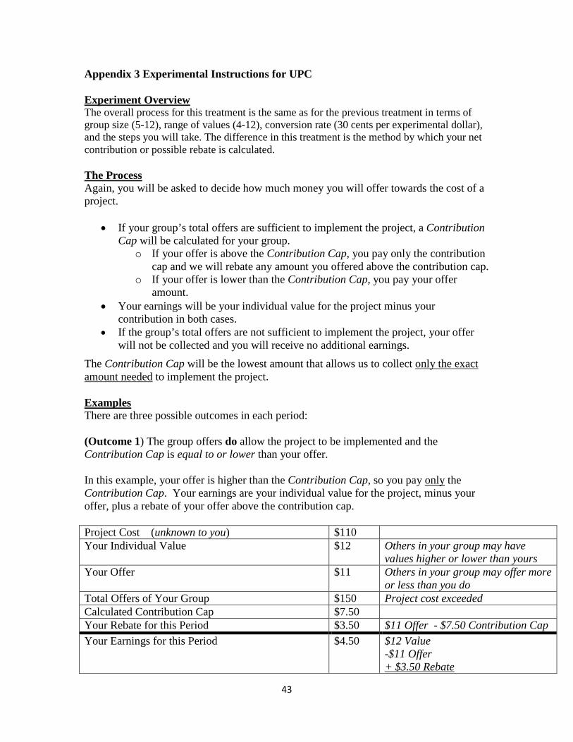
43

Appendix 3 Experimental Instructions for UPC


Experiment Overview


The Process

• If your group’s total offers are sufficient to implement the project, a Contribution

Cap will be calculated for your group. o If your offer is above the Contribution Cap, you pay only the contribution

cap and we will rebate any amount you offered above the contribution cap. o If your offer is lower than the Contribution Cap, you pay your offer

amount. • Your earnings will be your individual value for the project minus your

contribution in both cases. • If the group’s total offers are not sufficient to implement the project, your offer

will not be collected and you will receive no additional earnings.

The Contribution Cap will be the lowest amount that allows us to collect only the exact amount needed

to implement the project.


(Outcome 1) The group offers do allow the project to be implemented and the Contribution Cap is equal to or lower than your offer. In this example, your offer is higher than the Contribution Cap, so you pay only

the Contribution Cap. Your earnings are your individual value for the project, minus your offer, plus a rebate of your offer above the contribution cap.

Project Cost (unknown to you) $110 Your Individual Value $12 Others in your group may have


or less than you do Total Offers of Your Group $150 Project cost exceeded Calculated Contribution Cap $7.50 Your Rebate for this Period $3.50 $11 Offer - $7.50 Contribution Cap Your Earnings for this Period $4.50 $12 Value

-$11 Offer + $3.50 Rebate

44

= $4.50 Earnings

The Contribution Cap is lower than your offer. Even though you offered $11, you pay only the Contribution Cap of $7.50. Your earnings ($4.50) are your individual value ($12) minus your offer ($11), plus the rebate of your offer above the Contribution Cap ($3.50). (Outcome 2) The group offers do allow the project to be implemented and the Contribution Cap is higher than your offer. In this example, your offer is lower than the Contribution Cap, so your contribution is the full amount of your offer. Your earnings are your individual value for the project, minus your contribution. Project Cost (unknown to you) $80 Your Individual Value $11 Others in your group may have


or less than you do Total Offers of Your Group $100 Project cost exceeded Calculated Contribution Cap $9 Higher than your offer Your Earnings for This Period $10 $11 Value

=$10 Earnings - $1 Contribution (as Offered)

Your offer of $1 is lower than the Contribution Cap of $9, so you pay your offer amount. Your earnings ($10) are your individual value ($11) minus your contribution at your original offer amount ($1). (Outcome 3) The group offers do not allow the project to be implemented. In this example, your offer will not be collected and you will not receive any additional earnings. Project Cost (unknown to you) $100 Your Individual Value $12 Others in your group may have


or less than you do Total Offers of Your Group $85 Does not meet project cost Your Earnings for This Period $0 No additional value received The project cost is not met, so the project is not implemented. You do not receive your individual value for this period. Your $12 offer is not collected.

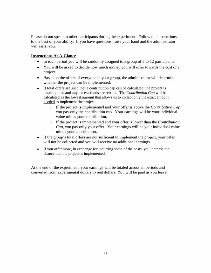
45

Please do not speak to other participants during the experiment. Follow the instructions to the best of your ability. If you have questions, raise your hand and the administrator will assist you.




• If total offers are such that a contribution cap can be calculated, the project is implemented and any excess funds are rebated. The Contribution Cap will be calculated as the lowest amount that allows us to collect only the exact amount needed

o If the project is implemented and your offer is above the Contribution Cap, you pay only the contribution cap. Your earnings will be your individual value minus your contribution.


o If the project is implemented and your offer is lower than the Contribution Cap, you pay only your offer. Your earnings will be your individual value minus your contribution.




46

Appendix 4 Experimental Instructions for UPA


Experiment Overview


The Process

• If your group’s total offers are sufficient to implement the project, a Uniform

Contribution will be calculated for your group. • If your offer is above the Uniform Contribution, you pay only the uniform

contribution and we will rebate any amount you offered above the uniform contribution. Your earnings will be your individual value for the project minus your contribution.

• If your offer is lower than the Uniform Contribution, you pay nothing. Your earnings will be your individual value for the project.

• If the group’s total offers are not sufficient to implement the project, your offer will not be collected and you will receive no additional earnings. .

The Uniform Contribution will be the lowest amount that allows us to collect only the exact amount needed



(Outcome 1) The group offers do allow the project to be implemented and the Uniform Contribution is equal to or lower than your offer. In this example, your offer is higher than the Uniform Contribution, so you pay only

Project Cost (unknown to you)

the Uniform Contribution. Your earnings are your individual value for the project, minus your offer, plus a rebate of your offer above the uniform contribution.

$110 Your Individual Value $12 Others in your group may have values

higher or lower than yours Your Offer $11 Others in your group may offer more

or less than you do Total Offers of Your Group $150 Project cost exceeded Calculated Uniform Contribution $7.50 Your Rebate for this Period $3.50 $11 Offer - $7.50 Contribution Your Earnings for This Period $4.50 $12 Value

-$11 Offer + $3.50 Rebate

47

= $4.50 Earnings

The Uniform Contribution is lower than your offer. Even though you offered $11, you pay only the Uniform Contribution of $7.50. Your earnings ($4.50) are your individual value ($12) minus your offer ($11), plus the rebate of your offer above the Uniform Contribution (3.50). (Outcome 2) The group offers do allow the project to be implemented and the Uniform Contribution is higher than your offer. In this example, your offer is lower than the Uniform Contribution, so you do not contribute. Your earnings are your individual value for the project. Project Cost (unknown to you) $80 Your Individual Value $11 Others in your group may have values


or less than you do Total Offers of Your Group $100 Project cost exceeded Calculated Uniform Contribution $9 Your Earnings for This Period $11 $11 Value

=$11 Earnings - $0 Contribution

Your offer of $1 is lower than the Uniform Contribution of $9, so you pay nothing. Your earnings ($11) are your individual value ($11). (Outcome 3) The group offers do not allow the project to be implemented. In this example, your offer will not be collected and you will not receive any additional earnings. Project Cost (unknown to you) $100 Your Individual Value $12 Others in your group may have values


or less than you do Total Offers of Your Group $85 Uniform contribution cannot be

calculated Your Earnings for This Period $0 No additional value received The project cost is not met, so the project is not implemented. You do not receive your individual value for this period. Your $12 offer is not collected.

48

Please do not speak to other participants during the experiment. Follow the instructions to the best of your ability. If you have questions, raise your hand and the administrator will assist you.




• If total offers are such that a uniform contribution can be calculated, the project is implemented and any excess funds are rebated. The Uniform Contribution will be calculated as the lowest amount that allows us to collect only the exact amount needed

o If the project is implemented and your offer is above the Uniform Contribution, you pay only the uniform contribution. Your earnings will be your individual value minus your contribution.


o If the project is implemented and your offer is lower than the Uniform Contribution, you pay nothing. Your earnings will be your individual value.




zwick center for food and resource policy - cag.uconn.edu · zwick center for food and resource...

Documents