zuse-institute berlin department optimization · outline 1 cutting planes in scip 2 cutting planes...
TRANSCRIPT

Cutting Planes in SCIP
Kati Wolter
Zuse-Institute BerlinDepartment Optimization
Berlin, 6th June 2007

Outline
1 Cutting Planes in SCIP
2 Cutting Planes for the 0-1 Knapsack Problem2.1 Cover Cuts2.2 Lifted Minimal Cover Cuts
3 Computational Results

Outline
1 Cutting Planes in SCIP
2 Cutting Planes for the 0-1 Knapsack Problem2.1 Cover Cuts2.2 Lifted Minimal Cover Cuts
3 Computational Results

SCIP
General cutting planes
. Complemented mixed integer rounding cuts
. Gomory mixed integer cuts
. Strong Chvátal-Gomory cuts
. Implied bound cuts
Cutting planes for special problems
. 0-1 knapsack problem
. 0-1 single node flow problem
. Stable set problem
I want to solve general MIPs!Why do I care about cutting planes for special problems?

General Cutting Plane Method
min{cT x : x ∈ X MIP} X MIP := {x ∈ Zn × Rm : Ax ≤ b}min{cT x : x ∈ X LP} X LP := {x ∈ Rn × Rm : Ax ≤ b}
Observation
. If the data are rational, thenI conv(X MIP) is a rational polyhedronI we can formulate the MIP as min{cT x : x ∈ conv(X MIP)}︸ ︷︷ ︸
LP

General Cutting Plane Method
min{cT x : x ∈ X MIP} X MIP := {x ∈ Zn × Rm : Ax ≤ b}min{cT x : x ∈ X LP} X LP := {x ∈ Rn × Rm : Ax ≤ b}
Observation
. If the data are rational, thenI conv(X MIP) is a rational polyhedronI we can formulate the MIP as min{cT x : x ∈ conv(X MIP)}︸ ︷︷ ︸
LP

General Cutting Plane Method
min{cT x : x ∈ X MIP} X MIP := {x ∈ Zn × Rm : Ax ≤ b}min{cT x : x ∈ X LP} X LP := {x ∈ Rn × Rm : Ax ≤ b}
Observation
. If the data are rational, thenI conv(X MIP) is a rational polyhedronI we can formulate the MIP as min{cT x : x ∈ conv(X MIP)}︸ ︷︷ ︸
LP
Problem (in general)
. Complete linear description of conv(X MIP)?
. Number of constraints needed to describe conv(X MIP) isextremely large

General Cutting Plane Method
min{cT x : x ∈ X MIP} X MIP := {x ∈ Zn × Rm : Ax ≤ b}min{cT x : x ∈ X LP} X LP := {x ∈ Rn × Rm : Ax ≤ b}
Observation
. If the data are rational, thenI conv(X MIP) is a rational polyhedronI we can formulate the MIP as min{cT x : x ∈ conv(X MIP)}︸ ︷︷ ︸
LP
Idea
. Construct a polyhedron Q withI conv(X MIP) ⊆ Q ⊆ X LP
I min{cT x : x ∈ conv(X MIP)} = min{cT x : x ∈ Q}
Start with X LP and add inequalities which are valid for X MIP
(but violated by the current LP solution) to X LP

Valid Inequalities for X MIP
. Inequalities valid for a relaxation of X MIP are valid for X MIP
. Generating valid inequalities for a relaxation is often easier
. The intersection of the relaxations should be a goodapproximation of X MIP
Relaxations of X MIP
1. Linear combinations of constraints defining X MIP
(row of the simplex tab., single constraint)2. Other information
I Logical implications between binary variables(conflict graph)
I Logical implications between a binary and a real variable

SCIP
General cutting planes
. Complemented mixed integer rounding cuts (Linear comb.)
. Gomory mixed integer cuts (Row of the simplex tab.)
. Strong Chvátal-Gomory cuts (Row of the simplex tab.)
. Implied bound cuts (Logical impl.)
Cutting planes for special problems
. 0-1 knapsack problem (Single constraint)
. 0-1 single node flow problem (Linear comb. and bounds)
. Stable set problem (Conflict graph)

Outline
1 Cutting Planes in SCIP
2 Cutting Planes for the 0-1 Knapsack Problem2.1 Cover Cuts2.2 Lifted Minimal Cover Cuts
3 Computational Results

0-1 Knapsack Polytope
conv(X BK ) X BK := {x ∈ {0, 1}n :∑j∈N
ajxj ≤ a0}
. N = {1, . . . , n}
. a0 and aj are integers for all j ∈ N
. aj > 0 for all j ∈ N(since binary variables can be complemented)
. aj ≤ a0 for all j ∈ N(since aj > a0 implies xj = 0)

Outline
1 Cutting Planes in SCIP
2 Cutting Planes for the 0-1 Knapsack Problem2.1 Cover Cuts2.2 Lifted Minimal Cover Cuts
3 Computational Results

Class of Cover Inequalities
Definition (Cover)
C ⊆ N .∑
j∈C aj > a0
Theorem
If C ⊆ N is a cover for X BK , then the cover inequality∑j∈C
xj ≤ |C| − 1
is valid for X BK .

Class of Cover Inequalities
Definition (Cover)
C ⊆ N .∑
j∈C aj > a0
Theorem
If C ⊆ N is a cover for X BK , then the cover inequality∑j∈C
xj ≤ |C| − 1
is valid for X BK .
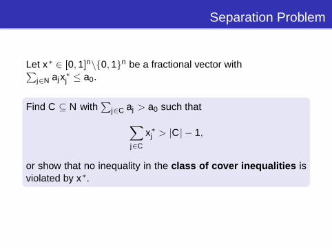
Separation Problem
Let x∗ ∈ [0, 1]n\{0, 1}n be a fractional vector with∑j∈N ajx∗
j ≤ a0.
Find C ⊆ N with∑
j∈C aj > a0 such that∑j∈C
x∗j > |C| − 1,
or show that no inequality in the class of cover inequalities isviolated by x∗.
The separation problem can be formulated as a 0-1 KP.

Separation Problem
Let x∗ ∈ [0, 1]n\{0, 1}n be a fractional vector with∑j∈N ajx∗
j ≤ a0.
Find C ⊆ N with∑
j∈C aj > a0 such that∑j∈C
x∗j > |C| − 1,
or show that no inequality in the class of cover inequalities isviolated by x∗.
The separation problem can be formulated as a 0-1 KP.

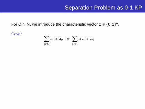
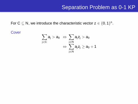
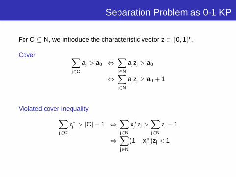
Separation Problem as 0-1 KP
For C ⊆ N, we introduce the characteristic vector z ∈ {0, 1}n.
Cover ∑j∈C
aj > a0 ⇔∑j∈N
ajzj > a0
⇔∑j∈N
ajzj ≥ a0 + 1
Violated cover inequality∑j∈C
x∗j > |C| − 1 ⇔∑j∈N
x∗j zj >∑j∈N
zj − 1
⇔∑j∈N
(1− x∗j )zj < 1

Separation Problem as 0-1 KP
For C ⊆ N, we introduce the characteristic vector z ∈ {0, 1}n.
Cover ∑j∈C
aj > a0
⇔∑j∈N
ajzj > a0
⇔∑j∈N
ajzj ≥ a0 + 1
Violated cover inequality∑j∈C
x∗j > |C| − 1 ⇔∑j∈N
x∗j zj >∑j∈N
zj − 1
⇔∑j∈N
(1− x∗j )zj < 1
Separation Problem as 0-1 KP
For C ⊆ N, we introduce the characteristic vector z ∈ {0, 1}n.
Cover ∑j∈C
aj > a0 ⇔∑j∈N
ajzj > a0
⇔∑j∈N
ajzj ≥ a0 + 1
Violated cover inequality∑j∈C
x∗j > |C| − 1 ⇔∑j∈N
x∗j zj >∑j∈N
zj − 1
⇔∑j∈N
(1− x∗j )zj < 1
Separation Problem as 0-1 KP
For C ⊆ N, we introduce the characteristic vector z ∈ {0, 1}n.
Cover ∑j∈C
aj > a0 ⇔∑j∈N
ajzj > a0
⇔∑j∈N
ajzj ≥ a0 + 1
Violated cover inequality∑j∈C
x∗j > |C| − 1 ⇔∑j∈N
x∗j zj >∑j∈N
zj − 1
⇔∑j∈N
(1− x∗j )zj < 1

Separation Problem as 0-1 KP
For C ⊆ N, we introduce the characteristic vector z ∈ {0, 1}n.
Cover ∑j∈C
aj > a0 ⇔∑j∈N
ajzj > a0
⇔∑j∈N
ajzj ≥ a0 + 1
Violated cover inequality∑j∈C
x∗j > |C| − 1
⇔∑j∈N
x∗j zj >∑j∈N
zj − 1
⇔∑j∈N
(1− x∗j )zj < 1

Separation Problem as 0-1 KP
For C ⊆ N, we introduce the characteristic vector z ∈ {0, 1}n.
Cover ∑j∈C
aj > a0 ⇔∑j∈N
ajzj > a0
⇔∑j∈N
ajzj ≥ a0 + 1
Violated cover inequality∑j∈C
x∗j > |C| − 1 ⇔∑j∈N
x∗j zj >∑j∈N
zj − 1
⇔∑j∈N
(1− x∗j )zj < 1
Separation Problem as 0-1 KP
For C ⊆ N, we introduce the characteristic vector z ∈ {0, 1}n.
Cover ∑j∈C
aj > a0 ⇔∑j∈N
ajzj > a0
⇔∑j∈N
ajzj ≥ a0 + 1
Violated cover inequality∑j∈C
x∗j > |C| − 1 ⇔∑j∈N
x∗j zj >∑j∈N
zj − 1
⇔∑j∈N
(1− x∗j )zj < 1

Separation Problem as 0-1 KP
For C ⊆ N, we introduce the characteristic vector z ∈ {0, 1}n.
Cover∑j∈N
ajzj ≥ a0 + 1
Violated cover inequality∑j∈N
(1− x∗j )zj < 1
x∗ satisfies all cover inequalities
⇔ ∀ z ∈ {0, 1}n with∑j∈N
ajzj ≥ a0 + 1 :∑j∈N
(1− x∗j )zj ≥ 1
⇔ min{∑j∈N
(1− x∗j )zj :∑j∈N
ajzj ≥ a0 + 1,
z ∈ {0, 1}n } ≥ 1
⇔ max{∑j∈N
(1− x∗j )zj :∑j∈N
aj zj ≤∑j∈N
aj − (a0 + 1),
z ∈ {0, 1}n } ≥ 1−∑j∈N
(1− x∗j )

Heuristic for the 0-1 KP
Input : c ∈ Qn+, a ∈ Qn
+\{0}, and b ∈ Q+
Output : Feasible solution of max{cT x : aT x ≤ b, x ∈ {0, 1}n}
1 Sort the indices such that c1a1≥ . . . ≥ cn
an
2 a ← 0
3 for j ← 1 to n do4 if a + aj ≤ b then5 xj ← 1
6 a ← a + aj
7 else8 while j ≤ n do9 xj ← 0
10 j ← j + 1
11 return x
Solves the LP relaxation and rounds down the solution.

Heuristic for the 0-1 KP
Input : c ∈ Qn+, a ∈ Qn
+\{0}, and b ∈ Q+
Output : Feasible solution of max{cT x : aT x ≤ b, x ∈ {0, 1}n}
1 Sort the indices such that c1a1≥ . . . ≥ cn
an
2 a ← 0
3 for j ← 1 to n do4 if a + aj ≤ b then5 xj ← 1
6 a ← a + aj
7 else8 while j ≤ n do9 xj ← 0
10 j ← j + 1
11 return x
Time complexity: O(n log n)

Exact Algorithm for the 0-1 KP
Input : c ∈ Qn+, a ∈ Zn
+\{0}, and b ∈ Z+
Output : Optimal solution of max{cT x : aT x ≤ b, x ∈ {0, 1}n}
Algorithm uses dynamic programming

Exact Algorithm for the 0-1 KP
Input : c ∈ Qn+, a ∈ Zn
+\{0}, and b ∈ Z+
Output : Optimal solution of max{cT x : aT x ≤ b, x ∈ {0, 1}n}
Algorithm uses dynamic programming
Time complexity: O(nb)

Practice
. A separator for cover cuts has only a limited effecton the overall performance of SCIP
. It seems to be important to separate strong cutting planes(facets or at least faces of reasonably high dimension)
Can we strengthen the cover inequalities?

Practice
. A separator for cover cuts has only a limited effecton the overall performance of SCIP
. It seems to be important to separate strong cutting planes(facets or at least faces of reasonably high dimension)
Can we strengthen the cover inequalities?

Outline
1 Cutting Planes in SCIP
2 Cutting Planes for the 0-1 Knapsack Problem2.1 Cover Cuts2.2 Lifted Minimal Cover Cuts
3 Computational Results

Class of Minimal Cover Inequalities
Definition (Minimal cover)
C ⊆ N.
∑j∈C aj > a0
.∑
j∈C\{i} aj ≤ a0 for all i ∈ C
Theorem
If C ⊆ N is a minimal cover for X BK , then theminimal cover inequality∑
j∈C
xj ≤ |C| − 1
defines a facet of
conv( X BK ⋂{x ∈ {0, 1}n : xj = 0 for all j ∈ N\C} ).

Class of Minimal Cover Inequalities
Definition (Minimal cover)
C ⊆ N.
∑j∈C aj > a0
.∑
j∈C\{i} aj ≤ a0 for all i ∈ C
Theorem
If C ⊆ N is a minimal cover for X BK , then theminimal cover inequality∑
j∈C
xj ≤ |C| − 1
defines a facet of
conv( X BK ⋂{x ∈ {0, 1}n : xj = 0 for all j ∈ N\C} ).

Sequential Up-Lifting
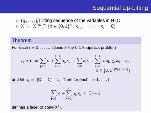
. (j1, . . . , jt) lifting sequence of the variables in N\C
. X i := X BK ⋂{x ∈ {0, 1}n : xji+1 = . . . = xjt = 0}

Sequential Up-Lifting
. (j1, . . . , jt) lifting sequence of the variables in N\C
. X i := X BK ⋂{x ∈ {0, 1}n : xji+1 = . . . = xjt = 0}
∑j∈C
xj ≤ |C| − 1 valid for X 0
∑j∈C
xj + αj1xj1 ≤ |C| − 1 valid for X 1
...∑j∈C
xj +t∑
k=1
αjk xjk ≤ |C| − 1 valid for X t = X BK
Sequential Up-Lifting
. (j1, . . . , jt) lifting sequence of the variables in N\C
. X i := X BK ⋂{x ∈ {0, 1}n : xji+1 = . . . = xjt = 0}
TheoremFor each i = 1, . . . , t , consider the 0-1 knapsack problem
zji = max{∑j∈C
xj +i−1∑k=1
αjk xjk :∑j∈C
ajxj +i−1∑k=1
ajk xjk ≤ a0 − aji ,
x ∈ {0, 1}|C|+(i−1)}
and let αji = (|C| − 1)− zji . Then for each i = 1, . . . , t ,
∑j∈C
xj +i∑
k=1
αjk xjk ≤ |C| − 1
defines a facet of conv(X i).

Sequential Up-Lifting
. (j1, . . . , jt) lifting sequence of the variables in N\C
. X i := X BK ⋂{x ∈ {0, 1}n : xji+1 = . . . = xjt = 0}
Different lifting sequences may lead to different inequalities!

Computing the Lifting Coefficients
. For each i = 1, . . . , t , solve the 0-1 KPI approximately (O(n log n))I exactly (O(nb))
. Zemel: Exact algo to calculate all lifting coefficients (O(n2))
I Uses dynamic programming to solve a reformulation of the0-1 KPs(role of the objective function and the constraint is reversed)

Practice
. Using sequential up-lifting to strengthen minimal cover cutsimproves the performance of SCIP
But, a separator which uses up- and down-lifting performs evenbetter!

Practice
. Using sequential up-lifting to strengthen minimal cover cutsimproves the performance of SCIP
But, a separator which uses up- and down-lifting performs evenbetter!

Class of Minimal Cover Inequalities
Theorem
If C ⊆ N is a minimal cover for X BK , then theminimal cover inequality∑
j∈C
xj ≤ |C| − 1
defines a facet of
conv( X BK ⋂{x ∈ {0, 1}n : xj = 0 for all j ∈ N\C} ).
Up-lifting: variables in N\C

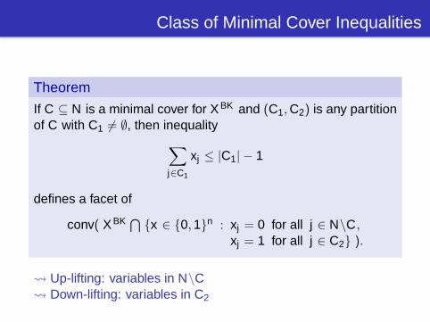
Class of Minimal Cover Inequalities
Theorem
If C ⊆ N is a minimal cover for X BK and (C1, C2) is any partitionof C with C1 6= ∅, then inequality∑
j∈C1
xj ≤ |C1| − 1
defines a facet of
conv( X BK ⋂{x ∈ {0, 1}n : xj = 0 for all j ∈ N\C,
xj = 1 for all j ∈ C2} ).
Class of Minimal Cover Inequalities
Theorem
If C ⊆ N is a minimal cover for X BK and (C1, C2) is any partitionof C with C1 6= ∅, then inequality∑
j∈C1
xj ≤ |C1| − 1
defines a facet of
conv( X BK ⋂{x ∈ {0, 1}n : xj = 0 for all j ∈ N\C,
xj = 1 for all j ∈ C2} ).
Up-lifting: variables in N\C Down-lifting: variables in C2

Sequential Up- and Down-Lifting
. Similar theorem as for sequential up-lifting
. Extension of Zemel’s up-lifting procedure can be used
. In SCIP, the separation problem for the class of liftedminimal cover inequalities using sequential up- anddown-lifting is solved heuristically

Outline of the Separation Algorithm
Step 1 (Cover)
. Determine a cover C for X BK
(separation problem for the class of cover inequalities)
Step 2 (Minimal cover and partition)
. Make the cover minimal by removing vars from C
. Find a partition (C1, C2) of C with C1 6= ∅
Step 3 (Lifting)
. Determine a lifting sequence of the variables in N\C1
. Lift the inequality∑
j∈C1xj ≤ |C1| − 1 using sequential up- and
down-lifting

Algorithmic Aspects
Step 1 (Cover)
. Which algorithm do we use to find the cover?
I Fixing of variablesI Modification of the separation problem (Gu et al. (1998))I Solving the separation problem exactly or approximately
Step 2 (Minimal cover and partition)
. In which order do we remove the variables?
. Which partition of the minimal cover do we use?
Step 3 (Lifting)
. Which lifting sequence do we use?
. Which algorithm do we use to solve the knapsack problems thatoccur in the sequential lifting procedure?

Resulting Algorithm
Step 1 (Cover)
. Fix all vars with x∗j = 0 to zero and all vars with x∗j = 1 to one
. Use the modification of the separation problem
. Solve the modified separation problem approximately
Step 2 (Minimal cover and partition)
. Nondecreasing order of x∗j and nondecreasing order of aj
. C2 := {j ∈ C : x∗j = 1} (|C1| = 1: change the partition)
Step 3 (Lifting)
. {j ∈ N\C : x∗j > 0}, C2, and then {j ∈ N\C : x∗j = 0}(nonincreasing order of aj )
. Use an extension of Zemel’s procedure

Important Aspects
Gap Closed % Sepa Time sec(Geom. Mean) (Total)
Value 4 Value 4
Default algorithm 16.31 0.00 1355.9 0.0
Cover – 1. modification 15.61 -0.70 7.6 -1348.3
Cover – 2. modification 16.42 0.11 7.1 -1348.8
Resulting algorithm 16.36 0.05 7.4 -1348.5
. Determination of the cover
I Solve the separation problem approximatelyI Modification of the separation problem

Important Aspects
Gap Closed % Sepa Time sec(Geom. Mean) (Total)
Value 4 Value 4
Default algorithm 16.31 0.00 1355.9 0.0
Cover – 1. modification 15.61 -0.70 7.6 -1348.3
Cover – 2. modification 16.42 0.11 7.1 -1348.8
Resulting algorithm 16.36 0.05 7.4 -1348.5
. Determination of the coverI Solve the separation problem approximately
I Modification of the separation problem

Important Aspects
Gap Closed % Sepa Time sec(Geom. Mean) (Total)
Value 4 Value 4
Default algorithm 16.31 0.00 1355.9 0.0
Cover – 1. modification 15.61 -0.70 7.6 -1348.3
Cover – 2. modification 16.42 0.11 7.1 -1348.8
Resulting algorithm 16.36 0.05 7.4 -1348.5
. Determination of the coverI Solve the separation problem approximatelyI Modification of the separation problem

Outline
1 Cutting Planes in SCIP
2 Cutting Planes for the 0-1 Knapsack Problem2.1 Cover Cuts2.2 Lifted Minimal Cover Cuts
3 Computational Results

Question
Comparison with other MIP solvers
. Are the cutting plane separators implemented inSCIP competitive to the ones included inother MIP solvers?

Computational Study
MIP solvers
. SCIP (CPLEX as LP solver)
. CPLEX
. COIN-OR Branch and Cut solver (COIN-OR LP solver)
Settings
. One cutting plane separator
. Isolated application
. Presolving disabled (used presolved instances obtained bythe presolving routines of CPLEX)
Test set
. 134 instances (MIPLIB 2003, MIPLIB 3.0, andMIP collection of Mittelmann)

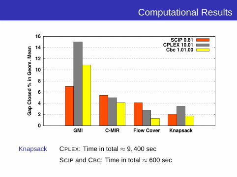
Computational Results
0
2
4
6
8
10
12
14
16
GMI C-MIR Flow Cover Knapsack
Gap
Clo
sed
% in
Geo
m. M
ean
SCIP 0.81CPLEX 10.01
Cbc 1.01.00
Performance measure Gap Closed % (100 · db−zLPzMIP−zLP
)
Computational Results
0
2
4
6
8
10
12
14
16
GMI C-MIR Flow Cover Knapsack
Gap
Clo
sed
% in
Geo
m. M
ean
SCIP 0.81CPLEX 10.01
Cbc 1.01.00
Knapsack CPLEX: Time in total ≈ 9, 400 sec
SCIP and CBC: Time in total ≈ 600 sec

Question
Impact on the overall performance of SCIP
. How strong is the impact of theindividual cutting plane separators on theoverall performance of SCIP?

Two Types of Tests
Impact of the individual cutting plane separators when they are used
as the only separators inSCIP
1. Started with runningSCIP without anyseparators
2. Compared theperformance with theone of SCIP when weenabled one separator
in connection with all otherseparators of SCIP
1. Started with runningSCIP with allseparators
2. Compared theperformance with theone of SCIP when wedisabled one separator

Enabling – Computational Study
Performance measures. Nodes. Time. Gap %
Improvement factor for each performance measure
Value for SCIP run without any separators
Value for SCIP run with one separator enabled
Factor by which enabling the separator improves theoverall performance (Factor > 1?)

Enabling – Computational Study
Performance measures. Nodes. Time. Gap %
Improvement factor for each performance measure
Value for SCIP run without any separators
Value for SCIP run with one separator enabled
Factor by which enabling the separator improves theoverall performance (Factor > 1?)

Enabling – Computational Results
0.5
1.0
1.5
2.0
2.5
3.0
3.5
C-MIR Flow Cover Knapsack GMI Impl. B. Clique
Impr
ovem
ent F
acto
r in
Geo
m. M
ean Nodes
TimeGap %

Disabling – Computational Study
Performance measures. Nodes. Time. Gap %
Degradation factor for each performance measure
Value for SCIP run with one separator disabled
Value for SCIP run with all separators
Factor by which disabling the separator degrades theoverall performance (Factor > 1?)

Disabling – Computational Study
Performance measures. Nodes. Time. Gap %
Degradation factor for each performance measure
Value for SCIP run with one separator disabled
Value for SCIP run with all separators
Factor by which disabling the separator degrades theoverall performance (Factor > 1?)

Disabling – Computational Results
0.5
1.0
1.5
2.0
C-MIR GMI Knapsack Flow Cover Impl. B. Clique
Deg
rada
tion
Fact
or in
Geo
m. M
ean Nodes
TimeGap %