zhanat zhanibekov - university of...

Final Year Project Report

School of Computer Science

University of Manchester

Data Mining Mining association rules

Zhanat Zhanibekov

Bsc Computing for Business Application

Supervisor: Ilias Petrounias

5th May 2010

2

Abstract

Nowadays, massive amount of data has been generated from various sources, including

industry, science and internet. As the amount of information grows exponentially, there is

need to efficiently process and extract valuable information using data mining technologies.

The aim of Data Mining is to extract hidden, predictive and potentially useful patterns from

large databases.9 This subject is becoming a very active research area and many different

methodologies have been produced to solve industrial and scientific problem.

The objective of this project is to research Association Rules Discovery field and describe the

process of developing software application, which extracts “useful patterns” from large

datasets using Apriori Algorithm. This paper discusses the software development process as

well as theoretical aspects of the project.

3

Acknowledgements

I would like to take this opportunity to thank my supervisor Ilias Petrounias for his assistance

and motivation throughout the project.

Also, I would like to thank my family and friends for their constant support.

4

Table of Content

Abstract ..................................................................................................................................... 2

Acknowledgements .................................................................................................................... 3

Tables of Figures ....................................................................................................................... 6

Chapter 1: Introduction ............................................................................................................ 7

1.1 Overview ..................................................................................................................... 7

1.2 Outline of the Problem ................................................................................................. 7 1.3 Project aims and objectives .......................................................................................... 7

1.4 Existing Data Mining system ....................................................................................... 8 1.5 Report Structure ........................................................................................................... 9

Chapter 2: Background .......................................................................................................... 10

2.1 Overview ....................................................................................................................10 2.2 Data Mining Motivation ..............................................................................................10

2.3 Data Mining Definition ...............................................................................................10 2.4 Knowledge Discovery in Databases ............................................................................11

2.5 Data Mining Methods .................................................................................................13 2.6 Data mining Challenges ..............................................................................................14

2.7 Summary ....................................................................................................................14

Chapter 3: Research................................................................................................................ 15

3.1 Overview ....................................................................................................................15

3.2 Association Rules Discovery .......................................................................................15 3.3 Problem Definition ......................................................................................................15

3.4 Association Rule Algorithm ........................................................................................16 3.5 Apriori Algorithm .......................................................................................................17

3.6 Rule Generation ..........................................................................................................18 3.7 Apriori algorithm improvements .................................................................................19

3.7.1 Hash-based techniques ......................................................................................... 19

3.7.2 Transaction reduction ........................................................................................... 19

3.7.3 Sampling.............................................................................................................. 19

3.7.4 Partitioning .......................................................................................................... 19

3.7.5 Dynamic Itemset Counting ................................................................................... 20

3.8 Advanced association rules techniques ........................................................................20

3.8.1 Generalized association rule ................................................................................. 20

3.8.2 Multiple-Level Association Rules ........................................................................ 21

3.8.3 Temporal Association Rule .................................................................................. 22

3.8.4 Quantitative Association Rules ............................................................................ 23

3.9 Summary ....................................................................................................................23

5

Chapter 4: Requirements and Design .................................................................................... 24

4.1 Overview ....................................................................................................................24 4.2 Software development methodology ...........................................................................24

4.3 Requirements definition ..............................................................................................25 4.4 Use Cases ...................................................................................................................27

4.5 System Overview Diagram..........................................................................................28 4.6 Activity Diagram ........................................................................................................30

4.7 Graphical User Interface Design..................................................................................30 4.8 Database Design .........................................................................................................32

4.9 Summary ....................................................................................................................33

Chapter 5: Implementation .................................................................................................... 34

5.1 Overview ....................................................................................................................34

5.2 Implementation tools ...................................................................................................34 5.2.1 Programming language ........................................................................................ 34

5.2.2 Database language ............................................................................................... 34

5.2.3 DBMS ................................................................................................................. 34

5.2.4 Development environment tools ........................................................................... 34

5.3 Data structure ..............................................................................................................35 5.4 Database Loader implementation ................................................................................36

5.5 Algorithm implementation ..........................................................................................38 5.6 Association mining rule example ................................................................................41

5.7 I/O association rules operation ....................................................................................44 5.8 Analyzer tool ..............................................................................................................44

5.9 Summary ....................................................................................................................45

Chapter 6: Testing and Evaluation ........................................................................................ 46

7.1 Overview ....................................................................................................................46

7.2 Testing Methods .........................................................................................................46 7.3 Unit and Functional Testing ........................................................................................46

7.4 Performance Testing ...................................................................................................47 7.5 Integration and System Testing ...................................................................................50

7.6 Evaluation ...................................................................................................................51 7.6.1 Development evaluation ....................................................................................... 51

7.6.2 System evaluation ................................................................................................ 52

7.6.3 Performance evaluation ........................................................................................ 52

7.7 Summary ....................................................................................................................52

Chapter 7: Conclusion ........................................................................................................... 53

7.1 Overview ....................................................................................................................53

7.2 Personal Experience ....................................................................................................53 7.3 Challenges ..................................................................................................................53

7.4 Further Improvements .................................................................................................54

References................................................................................................................................ 55

6

Tables of Figures

Figure 1: WEKA data mining software.................................................................................. 9

Figure 2: Data mining findings ............................................................................................ 10

Figure 3: KDD process ........................................................................................................ 11

Figure 4: CRISP-DM process .............................................................................................. 13

Figure 5. Market Basket transaction table ............................................................................ 15

Figure 6: Frequent itemset generation (Apriori algorithm) ................................................... 17

Figure 7: Rule generation in Apriori Algorithm29

................................................................ 18

Figure 8: Procedure ap-gerules(Fk, H1).29

............................................................................ 19

Figure 9: Concept hierarchy ................................................................................................ 20

Figure 10: Rational Unified Process .................................................................................... 25

Figure 11: Use case diagram for Data mining application .................................................... 28

Figure 12: System structure ................................................................................................. 29

Figure 13: Activity Diagram................................................................................................ 30

Figure 14: High fidelity prototype for GUI .......................................................................... 31

Figure 15: Transaction data in hash map.............................................................................. 35

Figure 16: Database connection ........................................................................................... 36

Figure 17: Database retrieves the tables ............................................................................... 37

Figure 18: Candidate selection process ................................................................................ 38

Figure 19: Algorithm processing ......................................................................................... 40

Figure 20: Generated rules displayed in the table ................................................................. 43

Figure 21: Saving results process ........................................................................................ 44

Figure 22: Comparing tool. ................................................................................................. 45

Figure 23: Relation of min support to the processing time ................................................... 49

Figure 24: Graphical representation of performance (items - candidate) .............................. 50

7

Chapter 1: Introduction

1.1 Overview This chapter gives an introduction of the project, describing the main goals and objective to

be achieved. Moreover, it shows the outline of the project, briefly describing each part.

1.2 Outline of the Problem For the last 20 years the amount of digital information has been greatly increased and

continues to grow exponentially.1 It is very hard to calculate the exact amount of digital

information in the world. The data is generated from sensors, internet, phones, cameras,

research laboratories so it requires more storage space. There are some examples where

processing of huge amount of information is involved.

In Switzerland, the experiment at the Large Hardon Collider at CERN’s particle-physics

laboratory produces 40 terabytes per second and the amount is much more that can be stored

in their data storages, so the scientist try to analyze it on the fly and the rest of the data is

removed. 2

In astronomy, in 2000 the telescope in Sloan Digital Sky Survey in New Mexico has been

acquired more data in the first few weeks than in whole history of astronomy. So for 10

years, the telescope produced approximately 140 terabytes of data. Moreover, in 2016 Large

Synoptic Survey Telescope in Chile will collect the same amount of data every 5 days. 3

Regarding the business area, Wall-Mart is the biggest retailer in the USA and it manages

more than 1 million transactions every hour. So it more than 2.5 petabytes (PB)i of data has

been stored in Wal-Mart databases.3

The study by International Data Corporation (IDC) shows that about 1200 exabytes (EB)ii of

digital information will be produced in 2010.4 The world has unimaginably huge amount of

data which offers new challenges and opportunities to people. The data analysis may identify

business trends, help to diagnose diseases, solve scientific problems and many more. On the

other hand, privacy and security protection will be harder to manage and extra storage and

processing technologies will be required.

The main problem is how to make the sense of the large amount of data. We produce too

much data, but have really small knowledge about it. The solution is to use special

technologies and methods to generate knowledge from data. This technology called “Data

Mining” and it was introduced in early 1990s.1

1.3 Project aims and objectives The main purpose of the project is to design and implement software application, which will

use association rule algorithm to mine data from databsae. Generally, the system should

i 1 PB =250 bytes

ii 1 EB = 260 bytes

8

perform following operation: scanning database for transactional data, applying association

rule algorithm on the “raw data” to extract “potentially useful” rules, which can be used by

business analytics.

There is the list of the objectives, which I need to achieve in order to develop the system.

1 The system should connect to any type of database, which will contain transactional

table, which has particular structure.

2 The Graphical User Interface should be intuitively simple to navigate and provide help

for the user in case he needs some.

3 Ensure that the system can handle large amount of data and process it for relatively short

period of time.

4 Provide the user an option to choose desired items for data mining process

5 Provide the feature to save the results of the mining process and open the files to view

generated association rules.

6 Develop the function to analyze and compare the results produced by the system.

1.4 Existing Data Mining system As far as the existing Data Mining products have been concerned, data mining marketplace

has been significantly grown over last decade. Rexeter analytics has been surveyed that, the

most popular area of data mining are CRM/Marketing, Academic, Finance and IT/Telecom.

Additionally, they found that the most widely used data mining techniques are regression,

decision trees and cluster analysis.5

There is the list of top 10 the most popular data mining products according to KKD nuggets

survey6:

1. SPSS/ SPSS Clementine

2. Salford Systems CART/MARS/TreeNet/RF

3. Rapid Miner

4. SAS

5. Angoss Knowledge Studio / Knowledge Seeker

6. KXEN

7. Weka

8. R

9. MS SQL

10. MATLAB

In order to start designing the application, author researched several existing data mining

system. Some of them had a great influence on the implementation decision taken during

development. For instance, WEKA project was comprehensively studied, because it has

similar set of features and was implemented using the same tools.

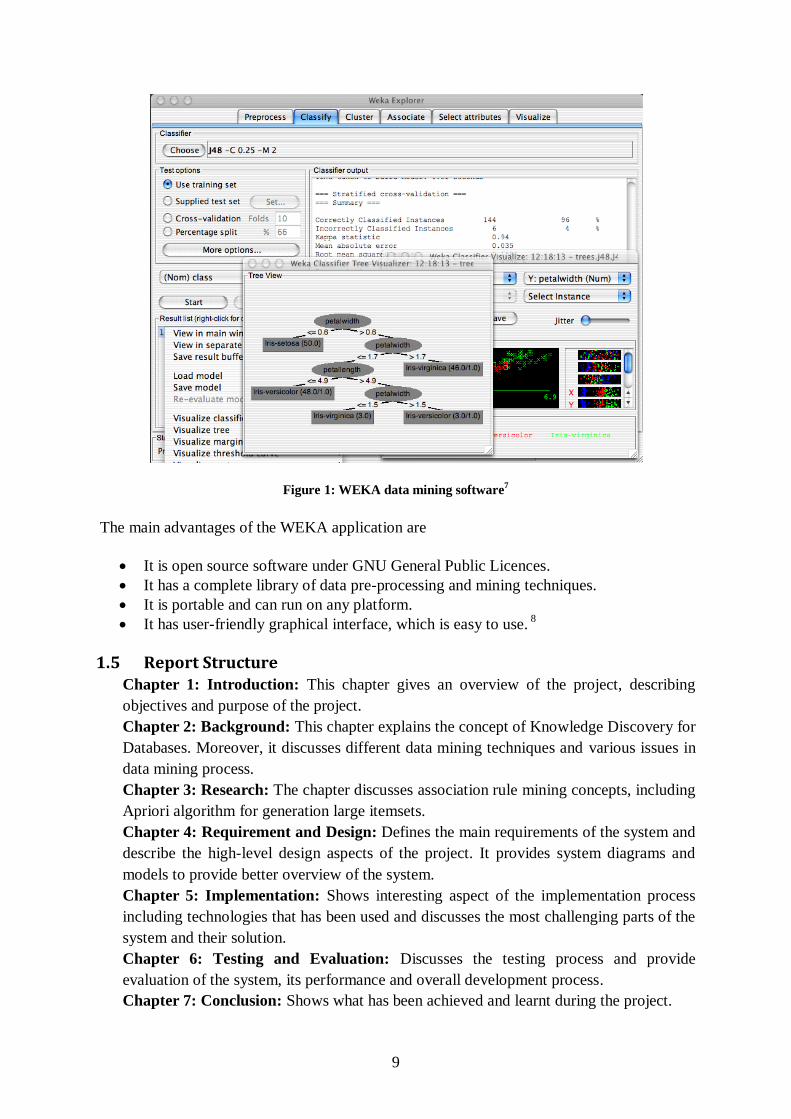
Regarding WEKA (Waikato Environment for Knowledge Analysis), it is open source

machine learning software which was written in Java. It can perform several data mining

techniques such as data pre-processing, clustering, association, classification, visualisation

etc. Figure 1 illustrates the classification analysis task and visualise the result using decision

tree.

http://www.the-data-mine.com/bin/view/Software/ANGOSSKnowledgeSTUDIO

http://www.the-data-mine.com/bin/view/Software/ANGOSSKnowledgeSEEKER

http://www.the-data-mine.com/bin/view/Software/KXEN

http://www.the-data-mine.com/bin/view/Software/Weka

http://www.the-data-mine.com/bin/view/Software/R

9

Figure 1: WEKA data mining software7

The main advantages of the WEKA application are

It is open source software under GNU General Public Licences.

It has a complete library of data pre-processing and mining techniques.

It is portable and can run on any platform.

It has user-friendly graphical interface, which is easy to use. 8

1.5 Report Structure Chapter 1: Introduction: This chapter gives an overview of the project, describing

objectives and purpose of the project.

Chapter 2: Background: This chapter explains the concept of Knowledge Discovery for

Databases. Moreover, it discusses different data mining techniques and various issues in

data mining process.

Chapter 3: Research: The chapter discusses association rule mining concepts, including

Apriori algorithm for generation large itemsets.

Chapter 4: Requirement and Design: Defines the main requirements of the system and

describe the high-level design aspects of the project. It provides system diagrams and

models to provide better overview of the system.

Chapter 5: Implementation: Shows interesting aspect of the implementation process

including technologies that has been used and discusses the most challenging parts of the

system and their solution.

Chapter 6: Testing and Evaluation: Discusses the testing process and provide

evaluation of the system, its performance and overall development process.

Chapter 7: Conclusion: Shows what has been achieved and learnt during the project.

10

Chapter 2: Background

2.1 Overview This chapter describes the role of data mining in business and outlines KDD processes and

different data mining techniques.

2.2 Data Mining Motivation Data Mining is the great tool when it comes to large amount of data. There are many reasons

to apply data mining such as it can reduce costs, increase revenue, improving customer and

user experience etc.

Nowadays, the business sector is very competitive and companies has to use the analytical

and data mining technologies to take leading position in their area. Moreover, the customer

has an access to greater amount of information about products in the internet and will go for

the better product or service. The top retailer will able to provide better customer service and

get more profit, as it has information about what customer more likely to buy as shown in

Figure 2.

Figure 2: Data mining findings

Currently, without Data Mining technologies companies would not get desired profit as they

may provide irrelevant offers and promote unwanted products or service to thir customer. As

the result, it may bring down customers satisfaction and cause reduction of the revenue.

2.3 Data Mining Definition As far as the “data mining” term has been concerned, there are various definition has been

made. However, some common characteristic can be identified.

Generally, data mining is the extraction/discovery of the hidden, potentially useful,

previously unknown patterns/relationship from the large data set.9

11

In analogy, we can make comparison with the gold mining, which is the process for the

sifting through large amount of ore to find valuable nuggets.

2.4 Knowledge Discovery in Databases Data Mining is the part of bigger process called knowledge discovery in databases. KDD has

been defined as “the non-trivial process of identifying novel, potentially useful and ultimately

understandable patterns in data.”10

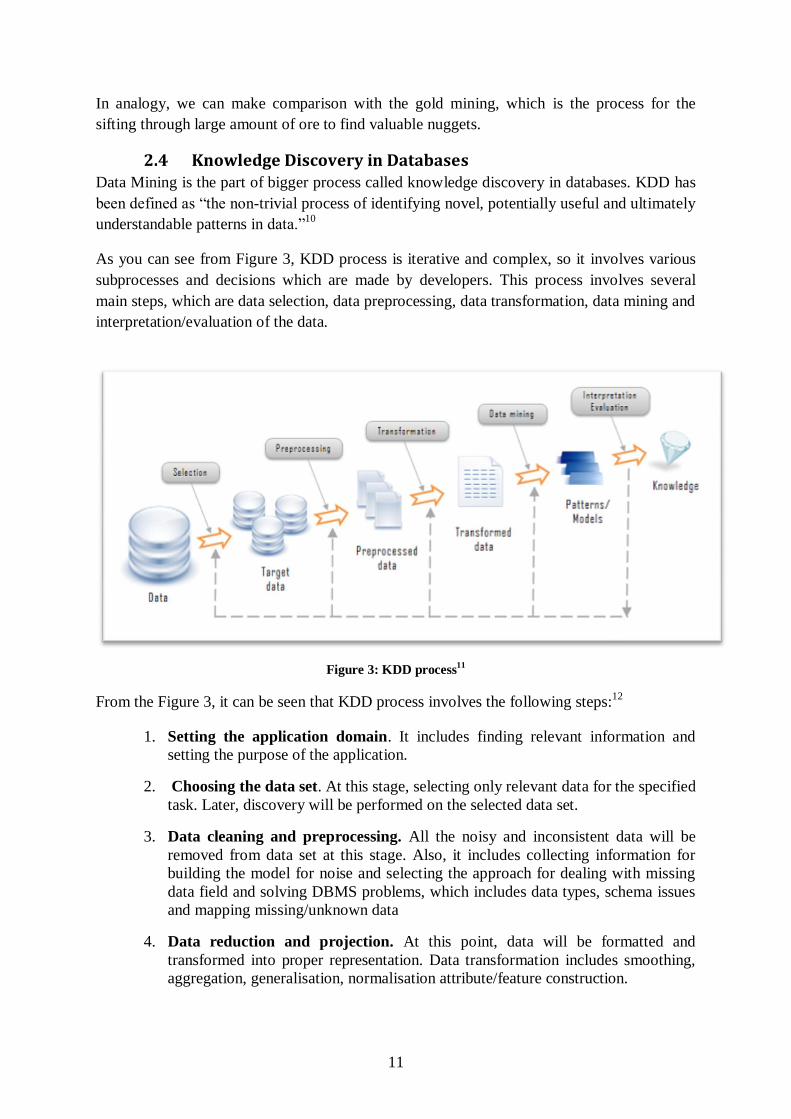
As you can see from Figure 3, KDD process is iterative and complex, so it involves various

subprocesses and decisions which are made by developers. This process involves several

main steps, which are data selection, data preprocessing, data transformation, data mining and

interpretation/evaluation of the data.

Figure 3: KDD process11

From the Figure 3, it can be seen that KDD process involves the following steps:12

1. Setting the application domain. It includes finding relevant information and

setting the purpose of the application.

2. Choosing the data set. At this stage, selecting only relevant data for the specified

task. Later, discovery will be performed on the selected data set.

3. Data cleaning and preprocessing. All the noisy and inconsistent data will be

removed from data set at this stage. Also, it includes collecting information for

building the model for noise and selecting the approach for dealing with missing

data field and solving DBMS problems, which includes data types, schema issues

and mapping missing/unknown data

4. Data reduction and projection. At this point, data will be formatted and

transformed into proper representation. Data transformation includes smoothing,

aggregation, generalisation, normalisation attribute/feature construction.

12

5. Selecting data mining functionality. According to the goal of the application

domain, the function of data mining will be chosen. The typical examples are

classification, association, clustering and so on.

6. Selecting Data Mining Algorithm. Due to the fact that user may pursue specific

aim from the data mining process; the particular algorithm for extracting pattern

should be selected. For instance, models for categorical data are different from the

numeric data

7. Apply Data Mining. Performing searching for interesting patterns and retrieving

the potentially useful results.

8. Interpretation and Evaluation. At this stage, retrieved information will be

represented on the human readable format and visualised. Evaluation includes

statistical validation and testing on importance, test on quality by the expert, pilot

survey for checking the accuracy of the model.

9. Using and utilizing knowledge. Finally the discovered knowledge will be used

for resolving business or scientific issues. Also the useful knowledge will be

documented and compared with other results.

There is another model for KDD process which has been developed by DaimlerChrysler,

SPSS and NCR in 1996. It is called “Cross Industry Standard Process for Data Mining” or

CRISP-DM and created for data mining processes in industry sector.13

The main purpose of

CRSIP-DM to make data mining project much faster and cheaper, as typical data mining

projects exceed the budget and do not meet deadlines. Moreover, the availability and quality

of the data has a direct affect on the data mining process performance. Therefore, we should

focus on the data analysis requirements and software design to minimize data mining effort.

Figure 4 shows the illustration of the CRISP-DM process, which is consisting of six main

phases. The arrows show the data flow between the phases. CRISP-DM process is highly

iterative model and phases may not correspond with the task, since it focuses on project

objectives and user requirements. It is quite common during the process the movement

between the phases as it helps to refine and improve the existing decision.

The first phase is Business Understanding, where we define business objectives, project

planning and identify data mining task. This is the most important and challenging part of the

project because the clear of understanding of the problem will produce better result.

Next stage is the Data Understanding stage. This stage includes analyzing the data and

applying advanced statistical method to it. For instance, if data will be retrieved from

different sources, we will need to integrate them dealing with data inconsistencies, missing

values and outliers. Once the data is understood, we start the data preparation phase, where

we transform raw data into readable format. Furthermore, Modeling phase starts where user

can choose the functionality of the data mining and specify mining algorithm.

After building and testing the model, we move to the evaluation step. During this process,

we decide whether or not to proceed with deployment of the model in the business

application. In other words, we check how well it satisfies the business objectives. Finally, in

deployment phase we integrate and document all the results of the data mining project.14

13

Figure 4: CRISP-DM process15

2.5 Data Mining Methods There are large amount of methods in data mining, we will discuss the most popular DM

technique such as classification, regression, clustering, sequence analysis and dependency

modeling.

Classification involves two stages. The first stage is supervising learning of a training set of

data to build the model. The second stage is the classification of data according to the model.

Some common examples are decision trees, neural network, Bayesian classification and k-

nearest neighbour classifier. Decision trees are top-down way of classification, when all data

is categories into leaf and node categories. Neural network is predictive approach, which is

based on the learning from prepared data set and use the learnt knowledge to the bigger data

set. Nearest neighbour learn the training set by identifying similarities of a group and use the

resultant data to process the test data.16

Regression applies formulas on the existing data and makes prediction based on results. For

instance, linear regression is the simplest form of regression and uses the straight line formula

(y = k*x + b) to finds the suitable values for k to predict the value of y, which is dependent

on x.17

Clustering groups a data into one or several category classes, which are not predefined and

must be created from the data. The building of category classes based on the similarity

metrics or probability density models. There are several types of clustering algorithms such

as hierarchical, partitional, density-based algorithm and so on. The common characteristics of

14

clustering algorithm that they require the number of clusters to produce in the input data set

before start of the algorithm. 18

Sequence analysis produce sequential patterns. The main objective of this method is to find

frequent sequences from data.19

Dependency modelling (or Association rules) describes the association between variables in

large data set. Market basket analysis is the most popular examples, where the technique can

be applied to discover the business trends and promote the products. Moreover, it is widely

used in web usage mining and bioinformatics.20

Summarization (characterization or generalization) group data into the subsets and provide

compact description for every set. Some advance techniques includes summary rules,

multivariate visualization techniques and functional relationship between variables. For

instance, this technique can be applied to automate reporting. 21

2.6 Data mining Challenges 1. Mining tasks and user interaction issues: These include issues related to the

knowledge mining at different granularities, knowledge representation and domain

knowledge appliance. 22

a. Incorporation of background knowledge

b. Mining various types of knowledge

c. Interactive mining

d. Removing noisy data and incomplete data

e. Visualisation of the mining result

f. Evaluation of the process and interestingness of the problem

2. Performance issues: This refers scalability, processing speed and parallelization of

data mining techniques. The algorithms should perform large amount of data for short

period of time. Due to large database size, computational complexity of data mining

algorithms and the broad distribution of sources, distrusted and parallel algorithm has

been developed to produce the greater performance result.22

3. Database compatibility issues: These include all issues with mining different types

of data from heterogeneous and global database systems. Data mining system should

able to handle relational and complex (hypertext, spatial, temporal or multimedia)

types of data. It is impossible to have one software application to effectively process

all kinds of data. Therefore, data mining tools should be specialised for mining

particular data types. Moreover, DM application must support the discovery from

different sources, integrating structured, semi-/un- structured information as

distributed and heterogeneous databases become widely used. For instance, Web

mining becomes a very challenging but can be very profitable area in data mining.22

2.7 Summary Due to the exponential growth of data collected from different sources (business, science,

industry etc), there is demand for effective data mining and analysis application. There are

numerous challenges concerning the effectiveness of data mining.

Data mining is extracting knowledge from large amount of data and it is part of bigger

process called knowledge discovery process. Finally, there is wide range of data mining

techniques, which were design for different purposes.

15

Chapter 3: Research

3.1 Overview In this chapter, we present methodology called association analysis and discuss its main

properties. Furthermore, Association rules algorithm implementation will be demonstrated

and corresponding examples will be illustrated. Finally, different types of rules will be

discussed.

3.2 Association Rules Discovery

As far as Association Rules has been concerned, it is technique for discovering interesting

relationship from the large data set. Association rules or sets of frequent item sets can

represent relationship between items. For instance, the association between two items can be

shown as the rule {Bread} {Butter}. It shows that there are strong dependencies between

Bread and Butter as the consumers more likely to buy these two items together.

Nowadays, this methodology has been applied in different areas, such as medical diagnosis,

web mining and telecommunication. In fact, one of the widely researched areas was “basket

market analysis”. 23

3.3 Problem Definition Regarding the “Market Basket Analysis”, it is the modeling technique which is use

association rules for prediction customer purchase behavior. Customer put some set of items

on their basket during their shopping process and software can register what kinds of

products are bought together. Finally, Marketers can apply this information to manage

inventory (selective inventory control), to promote their products (positioning items on the

particular place) and to conduct marketing campaign (targeting specific customer categories

and increasing customer satisfaction).24

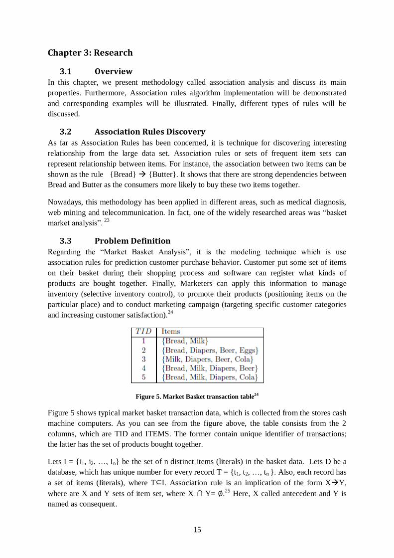
Figure 5. Market Basket transaction table24

Figure 5 shows typical market basket transaction data, which is collected from the stores cash

machine computers. As you can see from the figure above, the table consists from the 2

columns, which are TID and ITEMS. The former contain unique identifier of transactions;

the latter has the set of products bought together.

Lets I = {i1, i2, …, In} be the set of n distinct items (literals) in the basket data. Lets D be a

database, which has unique number for every record T = {t1, t2, …, tn }. Also, each record has

a set of items (literals), where T⊆I. Association rule is an implication of the form XY,

where are X and Y sets of item set, where X ∩ Y= ∅.25

Here, X called antecedent and Y is

named as consequent.

16

With respect to the measures of association rules, there are two essential measures called

support (S) and confidence (C).

Support (S) is the occurring frequency of the rule to the given data set, how often X and Y

appear together out of total number (N) of transactions.25

Support, S (XY) = Q(X ∩ Y)/N;

Example: Support of the relationship BreadMilk will be 60%, which is the number of how

often they are bought together (3 times) divided by total number of purchases (5

transactions).

Confidence (C) is the strength of the association, how often item in Y appear in transaction

that contain X. 25

Confidence, C (XY) = Q(X ∩ Y)/X;

Example: Let’s consider the rule Bread, Milk Diapers, the confidence of the rule will be

66%, as the combination of Bread, Milk and Diapers appears 2 times together and support of

Bread and Milk is equal to the 3. Therefore, the confidence is 2/3 = 0,6(6). 25

Lift (L) is ration between the confidence of the rules and support of the item set in the

consequent of the rule. The motivation that the high-confidence rule may be ambiguous since

it ignores the support of the item set in the rule consequent.

Lift = C (AB)/S (B);

Example: The Confidence of BreadMilk is 75%, and support of milk is 80%, then the lift

= 75/80 = 0.9375 (negative correlation). If Lift <1 then it is negative lift, otherwise it is

positive lift.

The lift has the same value as “interest factor” (I) for binary variables. It is the ratio of the

observed support to that expected by chance. 26

I (A, B) = S (A, B)/S (A)*S (B);

3.4 Association Rule Algorithm As for Association rule discovery, for each set of transaction T, discover all the rules where

support(S) is greater than minimum support threshold and confidence(C) is greater than

minimum confidence threshold.

The association rule algorithm consists of two steps:27

1. Frequent Itemset Generation: Extract all the itemset which occur with greater

frequency than the minimum support threshold. All this items will be called frequent

items.

2. Rule Generation: Generate all the high-confidence rules from the frequent itemset

generated on the first step. These rules will be called “strong rules”.

17

3.5 Apriori Algorithm With regard to frequent itemset generation implementation, Apriori is an influential algorithm

for learning association rules. It was introduced by Agrawal in 1994 and it pioneered the use

of support-based pruning to deal with exponential expansion of candidate item set.28

Pseudo code below demonstrates the process of frequent itemset generation of the Apriori

algorithm. Lets Ck is the set of candidate k-itemset. Lets Fk is set of frequent itemset.

Step 1-2: At the beginning, the algorithm runs through all data set and counts each item’s

support. Then it produces the F1 – the set of all frequent 1-itemset.

Step 3-5: Next, the algorithm iteratively produces new candidate k-item set, which is based

on previous iteration’s k-1 item set value. It uses Apriori-gen(Fk-1) functions to generate

candidate.

Step 6-11: After that, support of the candidate is calculated by passing over data set.

Additionally, all the candidate itemsets in CK in each transaction t is discovered by subset

function (subset (Ck, t)).

Step 12: Furthermore, all candidates which are not satisfy minimum support threshold

(minsup) will be removed and only frequent itemset will be left.

Step 13-14: If there is no new frequent itemset produced, then end algorithm (FK = ∅).Then

all frequent itemset will be joined for the rule generation process.

1: k = 1 2: Fk = {i | i ∈ I ∧ q({i}) ≥ N × minsup} //identify all large 1-itemset 3: repeat 4: k = k+1 5: Ck = apriori-gen(Fk-1). // produce candidate itemset 6: for each transaction t ∈ T do 7: Ct = subset (Ck, t). // find all candidates which is subset of t 8: for each candidate itemset c ∈Ct do 9: q(c) = q(c) + 1. 10: end for 11: end for 12: Fk = {c | c ∈ Ck ∧ q(c) ≥ N x minsup} // generate the large k-itemsets 13: until Fk = ∅ 14: Result = ∪Fk.

Figure 6: Frequent itemset generation (Apriori algorithm)29

Apriori-gen(Fk-1) is used to generate candidates item set. This function consists of two steps:

1. Candidate generation – Ck is generated by joining itself

2. Candidate Pruning – any (k-1) – itemset that is infrequent will be eliminated, as it

cannot be subset of a frequent k-itemset. It can minimize the number of candidate

itemset when support counted is performing.

18

Subset (Ck, t) – support counting function counts the number of occurrence of every

candidate in the database. It performed on all candidates that passed through Apriori-gen

(Fk-1). The effective way to implement this function is to count itemsets in each transaction

and refresh the value of support for corresponding candidate itemset.

3.6 Rule Generation With respect to rule generation, another task is to effectively extract association rule from the

frequent itemset. The algorithm applies level-wise techniqie for generating assoctiation rules.

In this appriach, each rule is positioned in particular level which has the same index as an

number of items in the rule consequent.

Figure 7 illustrates the pseudocde for rule generation. Initially, it process all the 1-item

consequence and store them in H1. Then it calls ap-gerules(Fk, H1), which is shown in figure

8. Finally, it terminates after all rules generated.

1: For each frequent k-itemset fk, k ≥ 2 do

2: H1 = {i | i ∈ fk}

3: call ap-genrules(fk, H1)

4: end for

Figure 7: Rule generation in Apriori Algorithm29

Step 1-2: count the size of frequent itemset k and size of rule consequent in m

Step 3: Condition is the size of frequent itemset is greater than the size of rule consequent. If

it satisfies, then continue to generate the rule. Otherwise, end this algorithm.

Step 4: Call ap-gerules(H1) to generate the new candidates for the association rule. The

method ap-gerules(H1) is similiar to that in frequent itemset generation.

Step 5- 12: For every rule, calcualte the confidence (conf) by dividing the support value

which were counted in frequent itemset generation.

Step 13: Method ap-gerules(Hm+1) is called to generate rules for the m+1 size of rule

consequent.

1: k = |fk| // frequent itemset size

2: m = |Hm| // rule consequent size

3: If k > m+1 then

4: Hm+1 = apriori-gen(Hm)

5: for each hm+1 ∈ Hm+1 do

6: conf = q(fk) / q(fk – hm+1)

7: if conf ≥ minconf then

8: output the rule (fk+1 - hm+1) hm+1

9: else

19

10: delete hm+1 from Hm+1

11: else if

12: end for

13: call ap-genrule(fk,Hm+1)

14 : end if Figure 8: Procedure ap-gerules(Fk, H1).

29

3.7 Apriori algorithm improvements

3.7.1 Hash-based techniques

This method can greatly reduce the size of the candidate k-itemsets examined. During the

scanning database process for generation frequent candidates from the 1-itemset, the 2-

itemsets will be generated. Next, 2-itemsets candidates will be stored (or hashed) into the

different buckets of a hash table. Then, related bucket counts will be added. If the 2-itemset

bucket count does not satisfy the minimum support, it will be eliminated from the candidate

set.30

3.7.2 Transaction reduction

This approach is based on decreasing the number of transaction processed in future iterations.

If transaction set does not have any large k-itemsets, then it also will not have any large (k+1)

– itemset. From this rule, corresponding transaction sets can be taken away from the future

iteration.30

3.7.3 Sampling

Sampling technique is used when the efficiency of the algorithm is prioritized. For instance, it

could be important for application running huge datasets regularly. Initially, from the

provided data D, sample data set S will be selected. Next, the large itemset from the S will be

generated, not from D.

The results of algorithm can be less accurate, because only S set is being searched for

frequent itemset and some global frequent itemset can be missed. The solution is to use the

lower minimum support value than minimum confidence to find local frequent itemset to S

(LS). Furthermore, the frequencies each itemset of in LS will be computed in the rest of the

database. This is used to identify if LS contain all global frequent itemset. Finally, if some

candidates are missed, the second scan will be performed in order to find all frequent

candidates. In the best case, only one scan is required in case all frequent candidates are

found.30

3.7.4 Partitioning

A partitioning technique requires only just 2 database scans in order to generate frequent

itemset. The process consists of two stages:

1. Database transaction (D) is split into n-nonoverlapping subset. The minimum support

for particular partitions will be result of multiplication of minimum support of D and

the number of transaction in that partition. In each partition the frequent itemset (local

20

frequent itemset) will be calculated. Furthermore, the local frequent itemset will be

stored in the special data structure, where for each itemset, corresponding TID’s of

transaction is stored. As the result, the database can be scanned only once.

2. In this stage, to identify global itemset, the actual support threshold for each itemset is

checked. The database is scanned only once, each partition can be stored in the main

memory.30

3.7.5 Dynamic Itemset Counting

The idea of this technique is that during the database scanning process, the candidate itemsets

will be added at any point. Initially, database is divided into the blocks, which is marked by

starting point. The support value is counted dynamically from the itemsets that has been

processed so far. If all subset of the itemset are frequents, the new candidates will be added

during the process. 30

3.8 Advanced association rules techniques This section discusses several techniques of association rule generation which involves more

complicated concepts those basic rules.

3.8.1 Generalized association rule

This type of association rules uses a concept of hierarchy that shows the set relationship

between various elements. This technique allows generating rules at different levels. The

definition of generalized association rules is almost similar to the regular association rules

XY, whereas it put constrains such as no item in Y may be above any item in X.31

As an example, Figure 9 shows a partial concept hierarchy for clothes. It can be seen that

white boots is the subtype of the boots and the boots is the subcategory of shoes. The

association rule Boots Shoes Cream has a lower support and confidence threshold that one

from the shoes, because the amount of transaction containing shoes is larger than number of

transactions, which contain Boots. Therefore, Black Boots Shoe Cream has a lower

support and confidence values than Shoes Shoe Cream.

Figure 9: Concept hierarchy

Clothes

Shoes

Slipper Derbys Boots

White Brown Black

Jeans Jackets Shorts T-Shirts

Crew Neck Raglan

21

There are several algorithms implemented to generate generalized rules. For instance,

transactions can be expanded by adding all items above it in any hierarchy.

3.8.2 Multiple-Level Association Rules

This type of association rules are subtype of Generalized Association Rules. It is association

rule, where each item has the set of relevant attributes. The set of multiple-level concepts are

represented by these attributes. 30

Table 1 illustrates the transaction table used in Multi-Level Association Rule. Here the

computer peripherals items can be described by “Category”, “Content” and “Brand”

attributes, which represents first-, second- and third-level concept respectively. Therefore,

each item in the transactional database, there are a set of domain values. Item in the database

can be described as “HP Laser printer”, if the “category”, “content” and “brand” columns

contain Printer, Laser and HP domain correspondingly.

Table 1: Transaction table

Category Content Brand

Printer Laser HP

Mouse Wireless Apple

… … …

Notebook 17 inch Sony Vaio

The main difference that itemset may be taken from any concept level in the hierarchy.

Therefore, Multiple-Level Association rules allow discovering more specific and concrete

knowledge from the data.

The concept of hierarchy can be traversed using top-down approach and frequent itemset can

be generated using variation of Apriori algorithm. After generating at level k, frequent

itemset can be produced in the next (k+1) level. Furthermore, frequent n-item set generated at

the first level in the concept hierarchy will be used as candidates to produce large n-itemset

for children on the further levels.

From the table above, it can be described as “Printer” is at the first concept level, “Laser

Printer” is at the second level and “HP Laser Printer” is at third level. Also, there are

minimum confidences and a support threshold specified for each level. 30

22

3.8.3 Temporal Association Rule

Temporal association rule is type of algorithm which also involves the discovery useful time-

related rules. It has a form of <AR, TF>, where AR is an association rule implication AB

and TF is the temporal feature which is contained in AR.32

Temporal feature TF state that

during each interval TP in f(TF), the existence of X in database transaction implies the

existence of Y in the same transaction.

1. AR has confidence C% in particular time period TP, TP∈F(x). For the confidence

C% of transaction in D (TP) that stores X also stores Y.

2. AR has support S% in particular time period TP, TP∈F(x). If for support S%, both X

and Y is stored in D (TP).

3. AR has temporal feature TF with rate R% in the database transaction D, if during at

least f% of the period of F (TP), it satisfy minimum confidence min_C% and

minimum min_S support 33

The examples of temporal feature can be specific period of time or some calendar time

expressions. For instance, “year*month (3-5)” can describe any spring period. The main

challenge of association rule implementation is that it is very costly to generate all the useful

rules due to two-dimensional solution space.

The example of the data mining transaction table is shown in the Figure below. It consists

from the 3 columns: transaction id, item name and time when transaction happened.

Table 2: Temporal transactional table

TID ITEM Date

10001 a, c, e, <*,01,09>

10002 a, d, e, f <*,02,09>

10003 d, e, f <*,02,09>

10004 a, d, e <*,05,09>

10005 a, b, c, d, f <*,05,09>

... ... ...

The main advantage of temporal association rules in the business is that many supermarkets

now have aisles dedicated to the sale of seasonal product.

23

3.8.4 Quantitative Association Rules

Regarding Quantitative Association Rules, this type combines both categorical and

quantitative data. This kind of rules contain continues attributes, which may reveal potentially

useful information in the business market. 31

The main advantage of this rule is that they provide more detailed results, as it extracts the

rules using multiples solution space.34

According to the internet survey, it is revealed that

“users whose annual salary is greater $120K belong to the 45-60 age groups”. This collected

data by internet survey is illustrated in the table below.35

Table 3:Quantitative transaction table35

Gender Age Annual

Income

Hours/week

using internet

Email account

quantity

Privacy

concerned

F 26 90K 20 4 +

M 51 135K 10 2 -

M 29 80K 10 3 +

F 45 120K 15 3 +

F 31 95K 20 5 +

M 25 55K 25 5 -

.. .. .. .. .. ..

3.9 Summary

In summary, basic concepts of association analysis has been discussed. Moreover, Apriori

algorithm has been reviewed in details and the related examples has been provided.

24

Chapter 4: Requirements and Design

4.1 Overview In this section, the specification and design of the application for mining association rules

will be described. Also the process of capturing and defining requirements will be explored.

Then different design solution and system structure will be illustrated to provide simpler

transition to implementation phase.

4.2 Software development methodology

As far as the software development process has been concerned, it describes the way for

designing, building and deploying software system.36

Therefore, it is important to select the

right development process before the start of the project. There were many different types of

models to choose from. However, the main criteria are to have flexible and open

methodology.

The Unified Process (UP) is well-known iterative methodology for building object oriented

software. Rational Unified Process is an example of the refinement of the Unified Process

and it is currently widely used in industry. Moreover, RUP process provides the best

practices into organized and well-structured process description.

Since RUP technique is an iterative process, development is structured into sequence of

short and time-boxed mini-projects called iteration. Iterations last about three weeks and it

includes its own requirement, analysis, implementation and evaluation procedures.

The main advantages of UP process include

1. Flexible, better productivity and early visible progress.

2. Research can be done within iteration so development process can be improved.

3. Early prevention of high risks, which includes technical, usability, design and other

issues, less project failure and lower defects probability.

4. Earlier feedbacks and user commitment results on closer meeting of requirement with

stakeholders.

25

Figure 10: Rational Unified Process37

As you can see from the Figure 8, Rational Unified Process has a cyclic form and consists

from several stages.

1. Requirement stage – capturing the system requirements

2. Design stage – planning and design the software structure

3. Implementation – coding and developing the system

4. Testing – examination the system and system evaluation.

5. Deployment – deployment and production

Each of these steps will be repeated iteratively until the final product release. Feedbacks are

provided and all material from the last workshop will be review and refined during each

iteration.

4.3 Requirements definition Regarding requirements analysis phase, it is vital to the success of the project. Requirement

analysis is the process of identifying and documenting user expectations for the new software

product.38

It discovers functionality, performance, usability and other characteristics of the

system.

The successful software is not “a program that works” but it is the program that meets the

client needs.39

Even if the program has the greatest features and does everything correct, but

does not meet the client expectation, it can be classified as failure. Hence, the right

identification of the requirements will greatly reduce the amount of work in further phases.

There are two types of requirements: functional and non-functional.

Non-functional requirements (NFR) - defines the how system must behave, the qualities of

the functionality of the system. (Examples: performance, availability, security, reliability,

usability etc.) It is essential for the system to be usable and accessible by the business

professionals, including those with visual impairments, such as color blindness. Furthermore,

it is vital that program will be reliable and store results in different format.

26

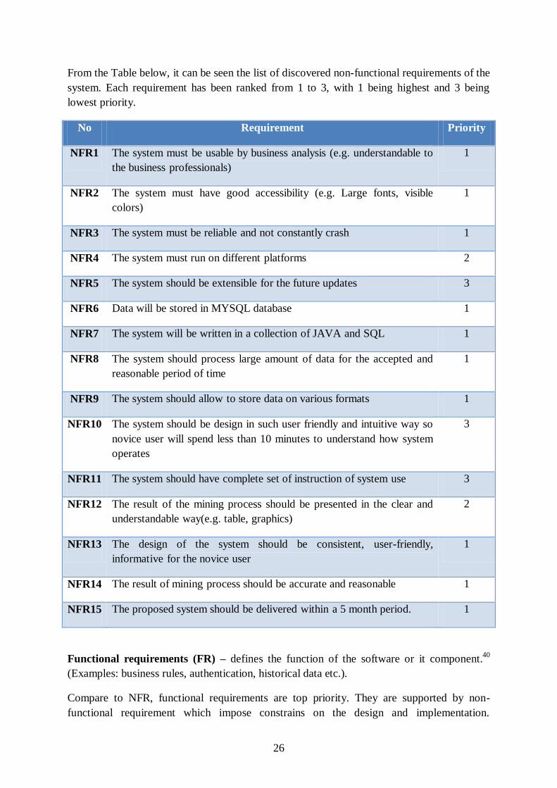
From the Table below, it can be seen the list of discovered non-functional requirements of the

system. Each requirement has been ranked from 1 to 3, with 1 being highest and 3 being

lowest priority.

No Requirement Priority

NFR1 The system must be usable by business analysis (e.g. understandable to

the business professionals)

1

NFR2 The system must have good accessibility (e.g. Large fonts, visible

colors)

1

NFR3 The system must be reliable and not constantly crash 1

NFR4 The system must run on different platforms 2

NFR5 The system should be extensible for the future updates 3

NFR6 Data will be stored in MYSQL database 1

NFR7 The system will be written in a collection of JAVA and SQL 1

NFR8 The system should process large amount of data for the accepted and

reasonable period of time

1

NFR9 The system should allow to store data on various formats 1

NFR10 The system should be design in such user friendly and intuitive way so

novice user will spend less than 10 minutes to understand how system

operates

3

NFR11 The system should have complete set of instruction of system use 3

NFR12 The result of the mining process should be presented in the clear and

understandable way(e.g. table, graphics)

2

NFR13 The design of the system should be consistent, user-friendly,

informative for the novice user

1

NFR14 The result of mining process should be accurate and reasonable 1

NFR15 The proposed system should be delivered within a 5 month period. 1

Functional requirements (FR) – defines the function of the software or it component.40

(Examples: business rules, authentication, historical data etc.).

Compare to NFR, functional requirements are top priority. They are supported by non-

functional requirement which impose constrains on the design and implementation.

27

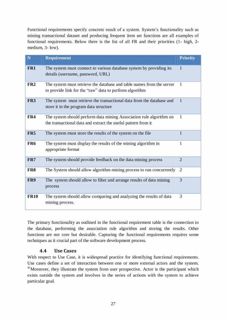
Functional requirements specify concrete result of a system. System’s functionality such as

mining transactional dataset and producing frequent item set functions are all examples of

functional requirements. Below there is the list of all FR and their priorities (1- high, 2-

medium, 3- low).

N Requirement Priority

FR1 The system must connect to various database system by providing its

details (username, password, URL)

1

FR2 The system must retrieve the database and table names from the server

to provide link for the “raw” data to perform algorithm

1

FR3 The system must retrieve the transactional data from the database and

store it in the program data structure

1

FR4 The system should perform data mining Association rule algorithm on

the transactional data and extract the useful pattern from it

1

FR5 The system must store the results of the system on the file 1

FR6 The system must display the results of the mining algorithm in

appropriate format

1

FR7 The system should provide feedback on the data mining process 2

FR8 The System should allow algorithm mining process to run concurrently 2

FR9 The system should allow to filter and arrange results of data mining

process

3

FR10 The system should allow comparing and analyzing the results of data

mining process.

3

The primary functionality as outlined in the functional requirement table is the connection to

the database, performing the association rule algorithm and storing the results. Other

functions are not core but desirable. Capturing the functional requirements requires some

techniques as it crucial part of the software development process.

4.4 Use Cases With respect to Use Case, it is widespread practice for identifying functional requirements.

Use cases define a set of interaction between one or more external actors and the system. 41

Moreover, they illustrate the system from user prospective. Actor is the participant which

exists outside the system and involves in the series of actions with the system to achieve

particular goal.

28

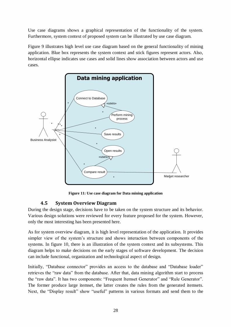
Use case diagrams shows a graphical representation of the functionality of the system.

Furthermore, system context of proposed system can be illustrated by use case diagram.

Figure 9 illustrates high level use case diagram based on the general functionality of mining

application. Blue box represents the system context and stick figures represent actors. Also,

horizontal ellipse indicates use cases and solid lines show association between actors and use

cases.

Business Analysist

Data mining application

*

*

Compare result

*

* Save results

Perform mining

process

*

*

*

*

*

*

Open results

Market researcher* *

«uses»

«uses»

Connect to Database

Figure 11: Use case diagram for Data mining application

4.5 System Overview Diagram During the design stage, decisions have to be taken on the system structure and its behavior.

Various design solutions were reviewed for every feature proposed for the system. However,

only the most interesting has been presented here.

As for system overview diagram, it is high level representation of the application. It provides

simpler view of the system’s structure and shows interaction between components of the

systems. In figure 10, there is an illustration of the system context and its subsystems. This

diagram helps to make decisions on the early stages of software development. The decision

can include functional, organization and technological aspect of design.

Initially, “Database connector” provides an access to the database and “Database loader”

retrieves the “raw data” from the database. After that, data mining algorithm start to process

the “raw data”. It has two components: “Frequent Itemset Generator” and “Rule Generator”.

The former produce large itemset, the latter creates the rules from the generated itemsets.

Next, the “Display result” show “useful” patterns in various formats and send them to the

29

“File buffer”, which operates with text file performing read/write functionality. Finally,

“Compare tool” can be used for analyzing and comparing data mining results.

System

Database

Connector

Rule

Generator

Frequent

Itemset

Generator

File buffer

Compare tool

Database

Loader

Display result

Database

FILE

Figure 12: System structure

30

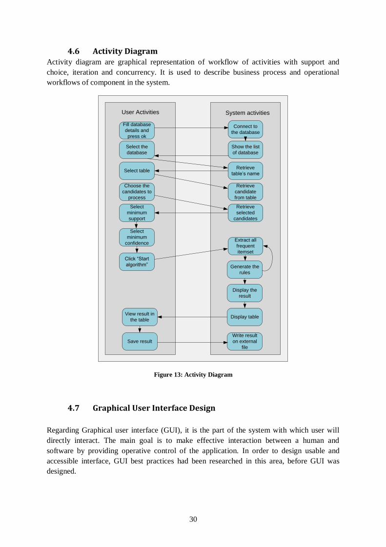
4.6 Activity Diagram Activity diagram are graphical representation of workflow of activities with support and

choice, iteration and concurrency. It is used to describe business process and operational

workflows of component in the system.

Show the list

of database

Fill database

details and

press ok

Connect to

the database

Select table

Retrieve

candidate

from table

Select the

database

User Activities System activities

Choose the

candidates to

process

Retrieve

selected

candidates

Select

minimum

support

Select

minimum

confidence

Click “Start

algorithm”

View result in

the table

Save result

Extract all

frequent

itemset

Generate the

rules

Display the

result

Display table

Write result

on external

file

Retrieve

table’s name

Figure 13: Activity Diagram

4.7 Graphical User Interface Design

Regarding Graphical user interface (GUI), it is the part of the system with which user will

directly interact. The main goal is to make effective interaction between a human and

software by providing operative control of the application. In order to design usable and

accessible interface, GUI best practices had been researched in this area, before GUI was

designed.

31

As the result, “Ten usability heuristics” by Jacob Nielsen was taken as basis for designing the

user interface. There are ten user interface design principles which was applied for my

application42

1. Visibility of system status – keep user informed about system processes.

2. Match between system and real world – words, phrases and labels must be familiar

to user.

3. User control and freedom – provide easer navigation for user.

4. Consistency and standard – provide intuitive design.

5. Error prevention – simple handling of error.

6. Recognition rather than recall – provide instructions in simple way.

7. Flexible and effective use – run several functions at one time.

8. Aesthetic and minimalist design – information should be provided where it required.

9. Help for user for error prevention – error message should be provided in plain

format.

10. Help and documentation – provide help about the system.

The picture bellow demonstrates the high fidelity prototype of mining application’s user

interface. To come up to this interface, various low fidelity interface prototypes were

sketched out by comparing at different existing software interfaces. Finally, the different

graphical features were analyzed and the best design solutions were deployed.

Figure 14: High fidelity prototype for GUI

32

From the figure below it can be seen that the system interface consists of four functional

areas. The main emphasis of GUI design was to make data mining process effective and

straightforward for business professionals. At the top of window will be menu bar (indicated

as 1), which contain file management and help information functions. On the left side, there

are control panel (indexed as 4), which provide tools for user to manipulate data mining

process. Bottom area contains panel which designed to provide feedback of data mining and

inform user about errors. Finally, on the center (indexed as 2) there is display area to show

the results of the mining process.

4.8 Database Design As database technology developing, modern databases are capable to store huge amount of

data. Sometimes they can reach Tera- or Petabytes and have a tendency to handle even more

data in the future.43

Therefore, data mining technologies must be able to deal with that

amount of time for reasonable time. For this purpose, the “raw data” should be preprocessed

and transformed into required format.

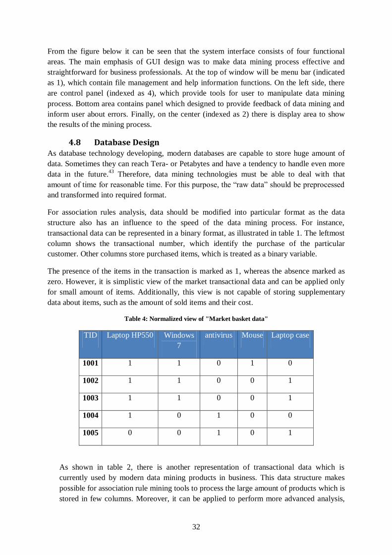
For association rules analysis, data should be modified into particular format as the data

structure also has an influence to the speed of the data mining process. For instance,

transactional data can be represented in a binary format, as illustrated in table 1. The leftmost

column shows the transactional number, which identify the purchase of the particular

customer. Other columns store purchased items, which is treated as a binary variable.

The presence of the items in the transaction is marked as 1, whereas the absence marked as

zero. However, it is simplistic view of the market transactional data and can be applied only

for small amount of items. Additionally, this view is not capable of storing supplementary

data about items, such as the amount of sold items and their cost.

Table 4: Normalized view of "Market basket data"

TID Laptop HP550 Windows

7

antivirus Mouse Laptop case

1001 1 1 0 1 0

1002 1 1 0 0 1

1003 1 1 0 0 1

1004 1 0 1 0 0

1005 0 0 1 0 1

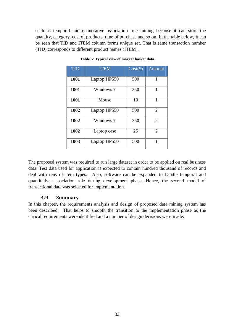
As shown in table 2, there is another representation of transactional data which is

currently used by modern data mining products in business. This data structure makes

possible for association rule mining tools to process the large amount of products which is

stored in few columns. Moreover, it can be applied to perform more advanced analysis,

33

such as temporal and quantitative association rule mining because it can store the

quantity, category, cost of products, time of purchase and so on. In the table below, it can

be seen that TID and ITEM column forms unique set. That is same transaction number

(TID) corresponds to different product names (ITEM).

Table 5: Typical view of market basket data

TID ITEM Cost($) Amount

1001 Laptop HP550 500 1

1001 Windows 7 350 1

1001 Mouse 10 1

1002 Laptop HP550 500 2

1002 Windows 7 350 2

1002 Laptop case 25 2

1003 Laptop HP550 500 1

The proposed system was required to run large dataset in order to be applied on real business

data. Test data used for application is expected to contain hundred thousand of records and

deal with tens of item types. Also, software can be expanded to handle temporal and

quantitative association rule during development phase. Hence, the second model of

transactional data was selected for implementation.

4.9 Summary In this chapter, the requirements analysis and design of proposed data mining system has

been described. That helps to smooth the transition to the implementation phase as the

critical requirements were identified and a number of design decisions were made.

34

Chapter 5: Implementation

5.1 Overview This chapter highlights the important aspects of system implementation, including the

technology choice, algorithm implementation and other interesting implementation solutions.

The main objective of this stage is to transform the design solutions into working model.

5.2 Implementation tools

5.2.1 Programming language

Regarding the programming languages, there is variety of different languages for

implementation has been considered. That is one of the key decisions in developing process

because using improper language can be de-motivating for writing better software. At times,

wrong choice can ruin the entire effort of software development.

Therefore, only few languages have been considered. These are Java, C/C++, Visual Basic

and Python. There are several factors have been taken into account while selecting the right

language such as the level of expertise, reference documentation and development platform.

Most of them offering similar features and some of them represent the leading edge

technology.

For following reasons Java was selected as the development language. It is mature in terms of

implementation as well as API. It is object-oriented and supports class loading, multi-

threading, garbage collection and database handling. Furthermore, the author had several

years of experiences in using Java.

5.2.2 Database language

For the database transaction, SQL (Structure Query Language) was selected. SQL is database

computer language used for organizing, managing and retrieving data from relational

database. The main advantages are reliability, performance, scalability and standardized.44

5.2.3 DBMS

Regarding database management system, MYSQL has been the primary choice because it has

consistent fast performance, high reliability and simple user interface.

5.2.4 Development environment tools

The main candidates for development environment choice were Netbeans and Eclipse.

However, NetBeans was preferred over the Eclipse for the some reason. Netbeans has more

intuitive and easy-to-use interface, sophisticated GUI builder editor, automatic integration of

framework. Moreover, Netbeans 6.8 version has improved performance compare to earlier

versions.

35

5.3 Data structure It is essential to use right data structure so it can be processed efficiently while performing

system operations. Initially, transaction data is stored in database as in Table 2. Since

application was design to perform basic Association rule, in this case, only the left two

column (TID and ITEM) need to be retrieved from database to the relevant data structures.

From the number of existing data structures, hash map was the best option to store

transactional data. Therefore itemset will be stored in the hash map as shown in Figure 15.

Figure 15: Transaction data in hash map.

The transaction id will be stored as key and itemset will be stored in corresponding array list.

It is very much like a hash table, except that Hash Map stucture is faster and thread-safe.

Also, Array List has been used while performing Apriori algorithm to store frequent item set.

As the result, the processing speed has been considerably increased.

1001

1002

1003

1004

1005

Laptop Windows 7 Mouse

Laptop Windows 7 Case

Laptop Windows 7 Case

Laptop Antivirus

Antivirus Case

TID (key) ITEM (Array List)

36

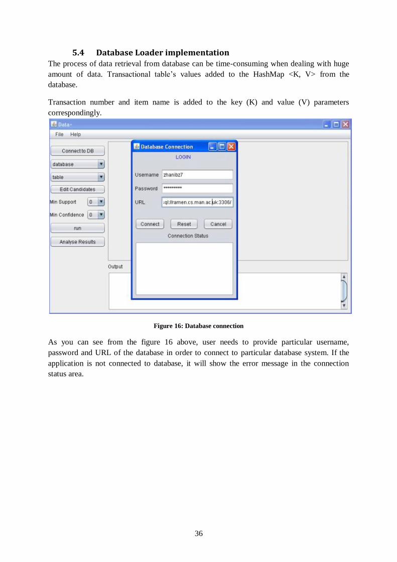
5.4 Database Loader implementation The process of data retrieval from database can be time-consuming when dealing with huge

amount of data. Transactional table’s values added to the HashMap <K, V> from the

database.

Transaction number and item name is added to the key (K) and value (V) parameters

correspondingly.

Figure 16: Database connection

As you can see from the figure 16 above, user needs to provide particular username,

password and URL of the database in order to connect to particular database system. If the

application is not connected to database, it will show the error message in the connection

status area.

37

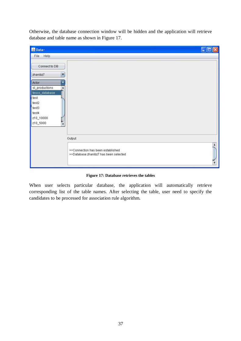
Otherwise, the database connection window will be hidden and the application will retrieve

database and table name as shown in Figure 17.

Figure 17: Database retrieves the tables

When user selects particular database, the application will automatically retrieve

corresponding list of the table names. After selecting the table, user need to specify the

candidates to be processed for association rule algorithm.

38

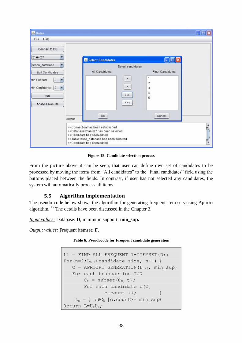
Figure 18: Candidate selection process

From the picture above it can be seen, that user can define own set of candidates to be

processed by moving the items from “All candidates” to the “Final candidates” field using the

buttons placed between the fields. In contrast, if user has not selected any candidates, the

system will automatically process all items.

5.5 Algorithm implementation The pseudo code below shows the algorithm for generating frequent item sets using Apriori

algorithm. 45

The details have been discussed in the Chapter 3.

Input values: Database: D, minimum support: min_sup.

Output values: Frequent itemset: F.

Table 6: Pseudocode for Frequent candidate generation

L1 = FIND ALL FREQUENT 1-ITEMSET(D);

For(n=2;Ln-1<candidate size; n++) {

C = APRIORI_GENERATION(Ln-1, min_sup)

For each transaction T∈D

Ct = subset(CK, t);

For each candidate c(Ct

c.count ++; }

Ln = { c∈Ck | c.count>= min_sup}

Return L=UkLk;

39

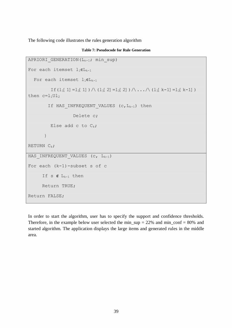
The following code illustrates the rules generation algorithm

Table 7: Pseudocode for Rule Generation

APRIORI_GENERATION(Ln-1; min_sup)

For each itemset ll∈Lk-1

For each itemset ll∈Lk-1

If(l1[1]=l2[1])/\(l1[2]=l2[2])/\.../\(l1[k-1]=l2[k-1])

then c=l1Ul2

If HAS_INFREQUENT_VALUES (c,Lk-1) then

Delete c;

Else add c to Ck;

}

RETURN Ck;

HAS_INFREQUENT_VALUES (c, Lk-1)

For each (k-1)-subset s of c

If s ∉ Lk-1 then

Return TRUE;

Return FALSE;

In order to start the algorithm, user has to specify the support and confidence thresholds.

Therefore, in the example below user selected the min_sup = 22% and min_conf = 80% and

started algorithm. The application displays the large items and generated rules in the middle

area.

40

Figure 19: Algorithm processing

Additionally, mining large datasets take some time, so user may perform another mining

operation simultaneously. From the image below it can be seen that user run several

algorithm at the same time. For instance, test, tesco_database and z10_10000 transactional

datasets were processed concurrently.

41

5.6 Association mining rule example This example illustrates how the algorithm is actually processes. Let’s consider database

consisting of 9 transactions. Let’s minimum confidence required is 80 % and minimum

support is 2(22%). Initially, Apriori algorithm will be applied to find frequent itemset.

Afterwards, Association rules will be generated support and confidence threshold.

Step 1: Generating frequent 1-itemsets.

In the beginning, database is scanned for the each item. Next, all unique candidates are

computed and their frequency of occurrence is calculated (support count). Furthermore,

candidates support count is compare with minimum support threshold.

TID ITEMS

1001 1, 2, 5

1002 2,4

1003 2,3

1004 1,2,4

1005 1,3

1006 2,3

1007 1,3

1008 1,2,3,5

1009 1,2,3

Itemset Support

count

1 6

2 7

3 6

4 2

5 2

Itemset Support

count

1 6

2 7

3 6

4 2

5 2

Step 2: Generate frequent 2-itemsets.

This step starts from generating 2-itemset candidate by joining the previous frequent 1-item

candidates. Then, 2-itemset candidate support count is calculated and compared to the

minimum support. If the support count does not satisfy the minimum support, the candidate

will be removed and will not be processed in the further steps. Therefore, only frequent set of

2-itemset will be processed

Count the

frequency

of each

candidate

by

scanning

D

Compare

support

count to

minimum

support

C1 L1 D

42

Itemset

1, 2

1, 3

1, 4

1, 5

2, 3

2, 4

2, 5

3, 4

3, 5

4, 5

Itemset Support

count

1, 2 4

1, 3 4

1, 4 1

1, 5 2

2, 3 4

2, 4 2

2, 5 2

3, 4 0

3, 5 1

4, 5 0

Itemset Support

count

1, 2 4

1, 3 4

1, 5 2

2, 3 4

2, 4 2

2, 5 2


This phase starts by joining the frequent set of 2-itemset into 3-itemset candidates. This

process involves the Apriori Property. The main idea of Apriori Property is if the itemset is

frequent, then all of its subset must also be frequent.

itemset

1 ,2, 3

1 ,2, 5

itemset Support

count

1, 2, 3 2

1, 2, 5 2

itemset Support

count

1, 2, 3 2

1, 2, 5 2


Similarly to the third step, algorithm generates a candidate set of 4-itemset. According to

Apriori property, the result of join {1, 2, 3, 5} is pruned, because its subset {2, 3, 5} is not

frequent. Finally, there are no frequent item sets generated as the result Apriori algorithm

terminates.

Eliminate

all

candidates

which does

not satisfy

minimum

support

C2 C2

Calculate

each

candidate

support

count

L2

Produce

candidate

itemset

from L1

Generate C3

candidate itemset

from L2

Count each

candidate Compare

min_sup with

support count

C3 C3 L3

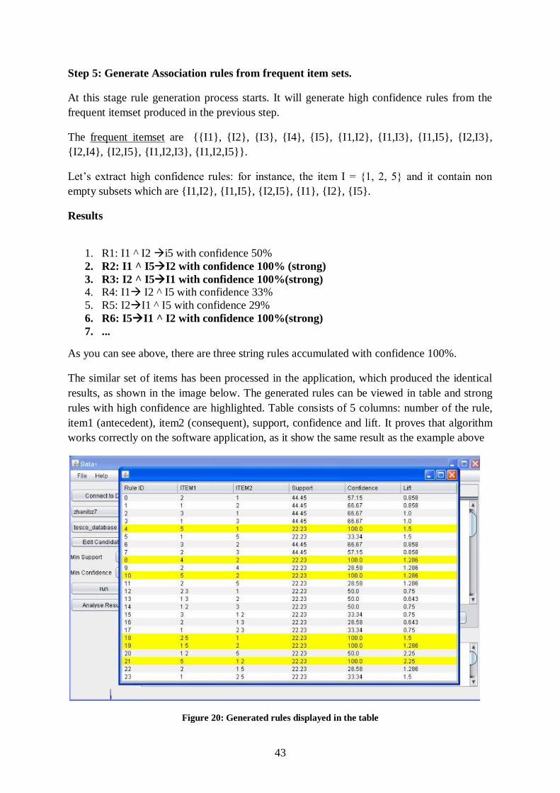
43

Step 5: Generate Association rules from frequent item sets.

At this stage rule generation process starts. It will generate high confidence rules from the

frequent itemset produced in the previous step.

The frequent itemset are {{I1}, {I2}, {I3}, {I4}, {I5}, {I1,I2}, {I1,I3}, {I1,I5}, {I2,I3},

{I2,I4}, {I2,I5}, {I1,I2,I3}, {I1,I2,I5}}.

Let’s extract high confidence rules: for instance, the item I = {1, 2, 5} and it contain non

empty subsets which are {I1,I2}, {I1,I5}, {I2,I5}, {I1}, {I2}, {I5}.

Results

1. R1: I1 ^ I2 i5 with confidence 50%

2. R2: I1 ^ I5I2 with confidence 100% (strong)

3. R3: I2 ^ I5I1 with confidence 100%(strong)

4. R4: I1 I2 ^ I5 with confidence 33%

5. R5: I2I1 ^ I5 with confidence 29%

6. R6: I5I1 ^ I2 with confidence 100%(strong)

7. ...

As you can see above, there are three string rules accumulated with confidence 100%.

The similar set of items has been processed in the application, which produced the identical

results, as shown in the image below. The generated rules can be viewed in table and strong

rules with high confidence are highlighted. Table consists of 5 columns: number of the rule,

item1 (antecedent), item2 (consequent), support, confidence and lift. It proves that algorithm

works correctly on the software application, as it show the same result as the example above

Figure 20: Generated rules displayed in the table

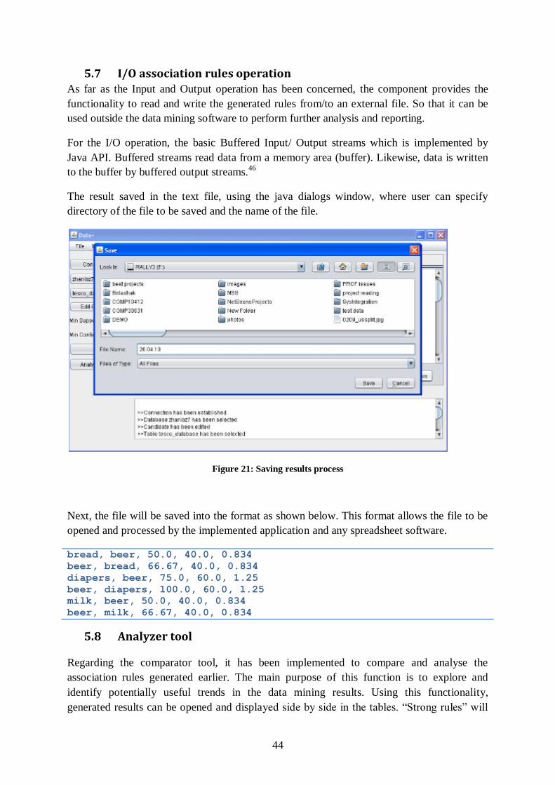
44

5.7 I/O association rules operation As far as the Input and Output operation has been concerned, the component provides the

functionality to read and write the generated rules from/to an external file. So that it can be

used outside the data mining software to perform further analysis and reporting.

For the I/O operation, the basic Buffered Input/ Output streams which is implemented by

Java API. Buffered streams read data from a memory area (buffer). Likewise, data is written

to the buffer by buffered output streams.46

The result saved in the text file, using the java dialogs window, where user can specify

directory of the file to be saved and the name of the file.

Figure 21: Saving results process

Next, the file will be saved into the format as shown below. This format allows the file to be

opened and processed by the implemented application and any spreadsheet software.

bread, beer, 50.0, 40.0, 0.834

beer, bread, 66.67, 40.0, 0.834

diapers, beer, 75.0, 60.0, 1.25

beer, diapers, 100.0, 60.0, 1.25

milk, beer, 50.0, 40.0, 0.834

beer, milk, 66.67, 40.0, 0.834

5.8 Analyzer tool

Regarding the comparator tool, it has been implemented to compare and analyse the

association rules generated earlier. The main purpose of this function is to explore and

identify potentially useful trends in the data mining results. Using this functionality,

generated results can be opened and displayed side by side in the tables. “Strong rules” will

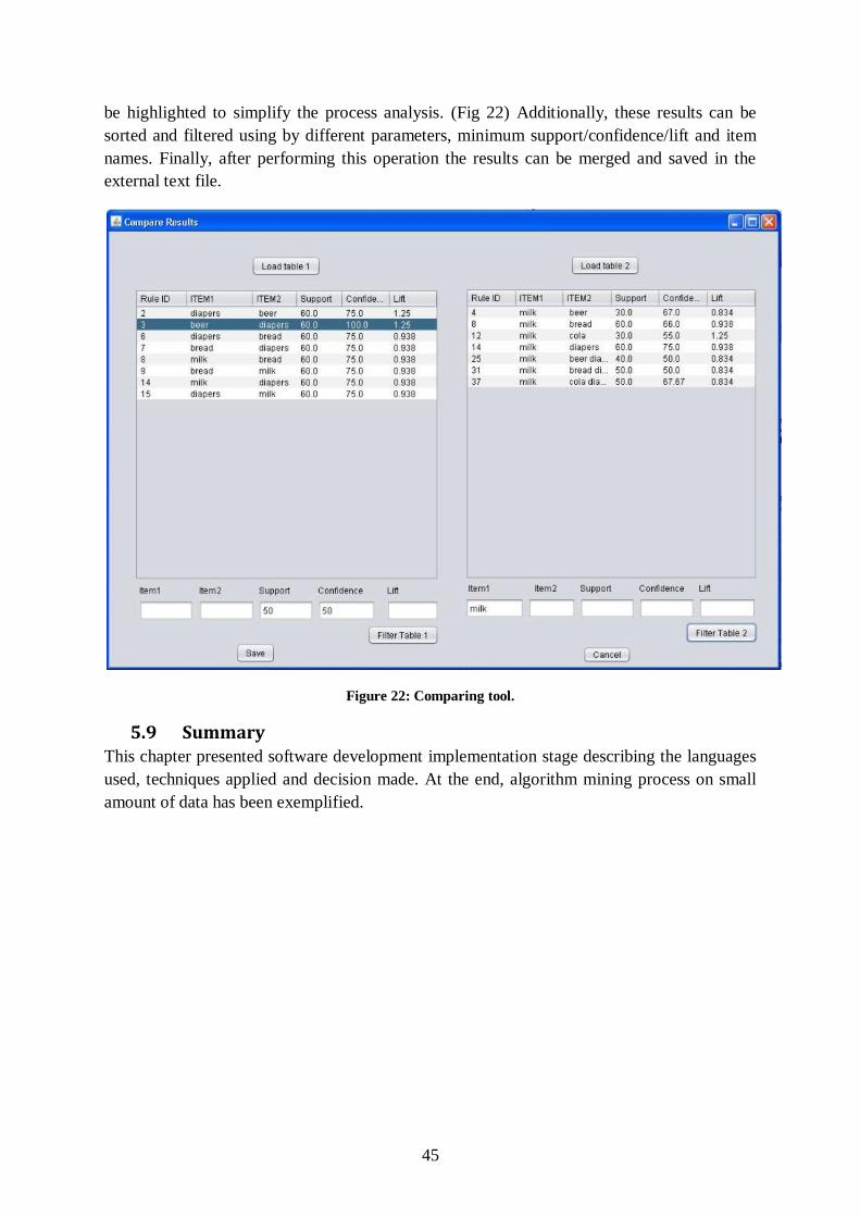
45

be highlighted to simplify the process analysis. (Fig 22) Additionally, these results can be

sorted and filtered using by different parameters, minimum support/confidence/lift and item

names. Finally, after performing this operation the results can be merged and saved in the

external text file.

Figure 22: Comparing tool.

5.9 Summary This chapter presented software development implementation stage describing the languages

used, techniques applied and decision made. At the end, algorithm mining process on small

amount of data has been exemplified.

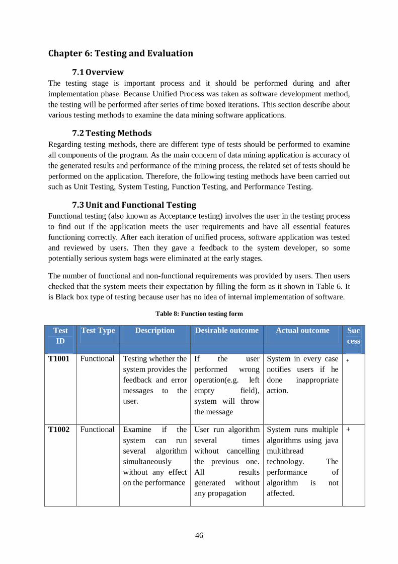
46

Chapter 6: Testing and Evaluation

7.1 Overview The testing stage is important process and it should be performed during and after

implementation phase. Because Unified Process was taken as software development method,

the testing will be performed after series of time boxed iterations. This section describe about

various testing methods to examine the data mining software applications.

7.2 Testing Methods

Regarding testing methods, there are different type of tests should be performed to examine

all components of the program. As the main concern of data mining application is accuracy of

the generated results and performance of the mining process, the related set of tests should be

performed on the application. Therefore, the following testing methods have been carried out

such as Unit Testing, System Testing, Function Testing, and Performance Testing.

7.3 Unit and Functional Testing Functional testing (also known as Acceptance testing) involves the user in the testing process

to find out if the application meets the user requirements and have all essential features

functioning correctly. After each iteration of unified process, software application was tested

and reviewed by users. Then they gave a feedback to the system developer, so some

potentially serious system bags were eliminated at the early stages.

The number of functional and non-functional requirements was provided by users. Then users

checked that the system meets their expectation by filling the form as it shown in Table 6. It

is Black box type of testing because user has no idea of internal implementation of software.

Table 8: Function testing form

Test

ID

Test Type Description Desirable outcome Actual outcome Suc

cess

T1001 Functional Testing whether the

system provides the

feedback and error

messages to the

user.

If the user

performed wrong

operation(e.g. left

empty field),

system will throw

the message

System in every case

notifies users if he

done inappropriate

action.

+

T1002 Functional Examine if the

system can run

several algorithm

simultaneously

without any effect

on the performance

User run algorithm

several times

without cancelling

the previous one.

All results

generated without

any propagation

System runs multiple

algorithms using java

multithread

technology. The

performance of

algorithm is not

affected.

+

47

Unit testing is carried out to check is particular module or unite of code is working correct

before integrating them into modules. The main advantage of unit test is prevention of system

defects in the early stages. Despite of Functional testing, the Unit test is the “White Box” as

developer has an access to the code. For particular components the test code has been written.

The examples of tested components are connecting to database, retrieving the candidates,

checking the filters etc. The database connection was validated in unit testing as shown on

table7.

Table 9: Functional testing

Test

ID

Test Type Description Desirable

outcome

Actual outcome Suc

cess

T1011 Unit Testing whether the

system can connect

to any type of

database. The

various database

details are

hardcoded.

Database

successfully

connects to any

database.

System connected to

the database. The

tested databases are

MYSQL, Heidi SQL

and Oracle database

+

7.4 Performance Testing Speed and efficiency of data mining process is key characteristics of any mining software

application. The amount of time, which algorithm spends on the data mining algorithm

should be reasonable. Therefore, the efficiency of the system can be evaluated by setting

different values of minimum support and measuring the amount of time required to generate

the association rules.

In order to evaluate the system performance, the synthetic datasets were created. It has been

decided to generate several sets of data with different number of records. Then values of

minimum support will be incremented up to specific point to analyze the effect of changing

support value to the system performance. The test data will have the same structure as the

dataset used in implementation phase. Similarly, the table will contain the two fields:

transaction id (TID) and item name (ITEM).

Since the main concern is to get comprehensive view of system mining performance, the

synthetic datasets were generated. Therefore test dataset D10000 of 10000 records and its

subset D5000 of 5000 records has been generated by Spawner software47

and then

preprocessed manually into required format.

It has been decided to test data mining application using 2 different approaches. The first way

is to process each test dataset separately to analyze the maximum performance. The second

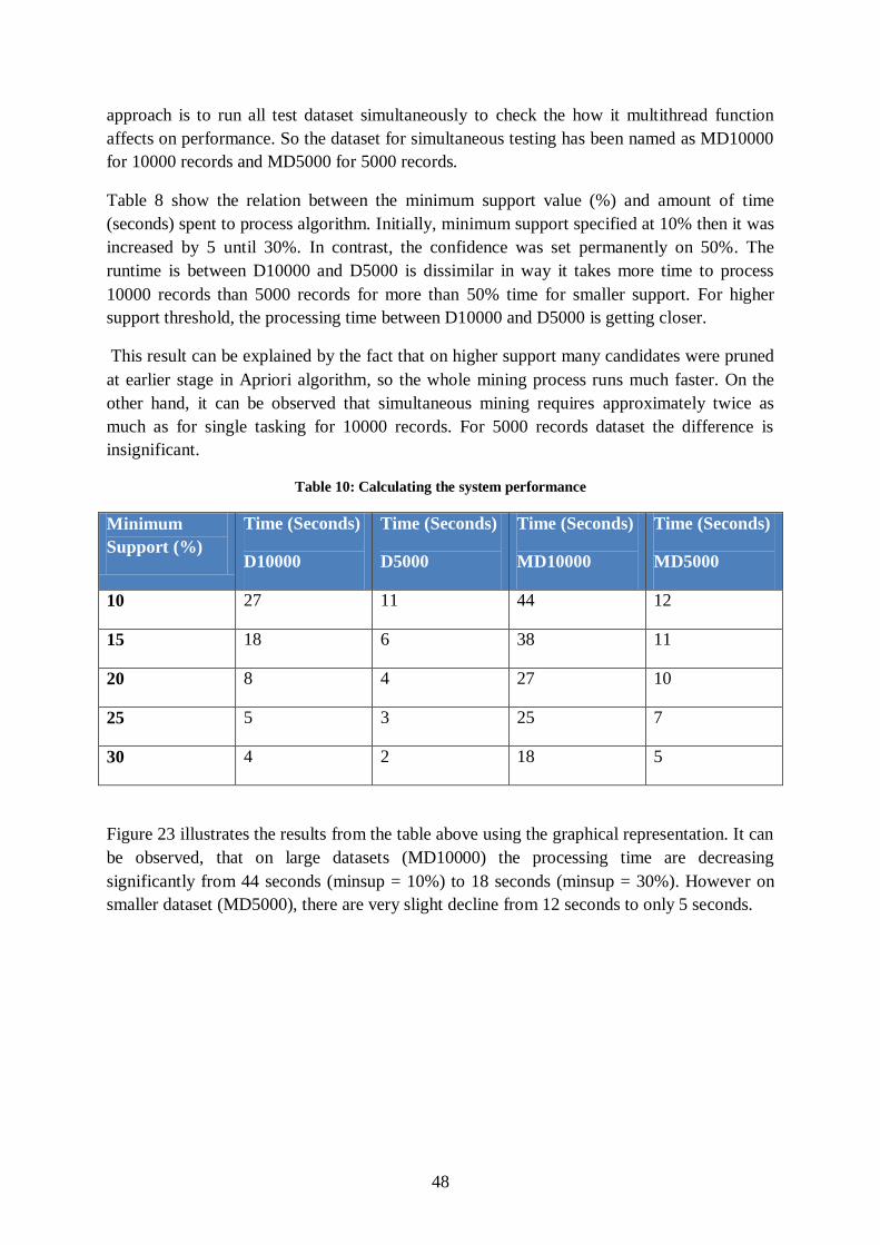
48

approach is to run all test dataset simultaneously to check the how it multithread function

affects on performance. So the dataset for simultaneous testing has been named as MD10000

for 10000 records and MD5000 for 5000 records.

Table 8 show the relation between the minimum support value (%) and amount of time

(seconds) spent to process algorithm. Initially, minimum support specified at 10% then it was

increased by 5 until 30%. In contrast, the confidence was set permanently on 50%. The

runtime is between D10000 and D5000 is dissimilar in way it takes more time to process

10000 records than 5000 records for more than 50% time for smaller support. For higher

support threshold, the processing time between D10000 and D5000 is getting closer.

This result can be explained by the fact that on higher support many candidates were pruned

at earlier stage in Apriori algorithm, so the whole mining process runs much faster. On the

other hand, it can be observed that simultaneous mining requires approximately twice as

much as for single tasking for 10000 records. For 5000 records dataset the difference is

insignificant.

Table 10: Calculating the system performance

Minimum

Support (%)

Time (Seconds)

D10000

Time (Seconds)

D5000

Time (Seconds)

MD10000

Time (Seconds)

MD5000

10 27 11 44 12

15 18 6 38 11

20 8 4 27 10

25 5 3 25 7

30 4 2 18 5

Figure 23 illustrates the results from the table above using the graphical representation. It can

be observed, that on large datasets (MD10000) the processing time are decreasing

significantly from 44 seconds (minsup = 10%) to 18 seconds (minsup = 30%). However on

smaller dataset (MD5000), there are very slight decline from 12 seconds to only 5 seconds.

49

Figure 23: Relation of min support to the processing time

As for candidate-related performance experiment, the processing time for mining various

numbers of items has been calculated. For this purpose, the large transactional datasets has

been generated of size 141272 (LD1) and 54000 records (LD2), so the application was tested

on real like data.

Table 11: Relation between number of candidates and processing time

Number of candidates Time(seconds) on LD1 Time(seconds) LD2

20 46 38

16 44 37

12 41 35

8 38 33

4 26 23

The table above provides the experimental results obtained by processing various numbers of

unique items from LD1 and LD2 datasets. It consists of 3 columns: number of items involved

in processing, time spent on processing 141272 records and time taken for 54000 records.

The support and confidence thresholds were set on 30% and 50% respectively. The number

of candidates was increased from 4 to 20 items by 4 candidates at each test. As the table 9

shows, there is minor difference in time for processing LD1 and LD2. A possible explanation

0

5

10

15

20

25

30

35

40

45

50

10 15 20 25 30

Tim

e(S

eco

nd

s)

Minimum Support(%)

D10000

D5000

MD10000

MD5000

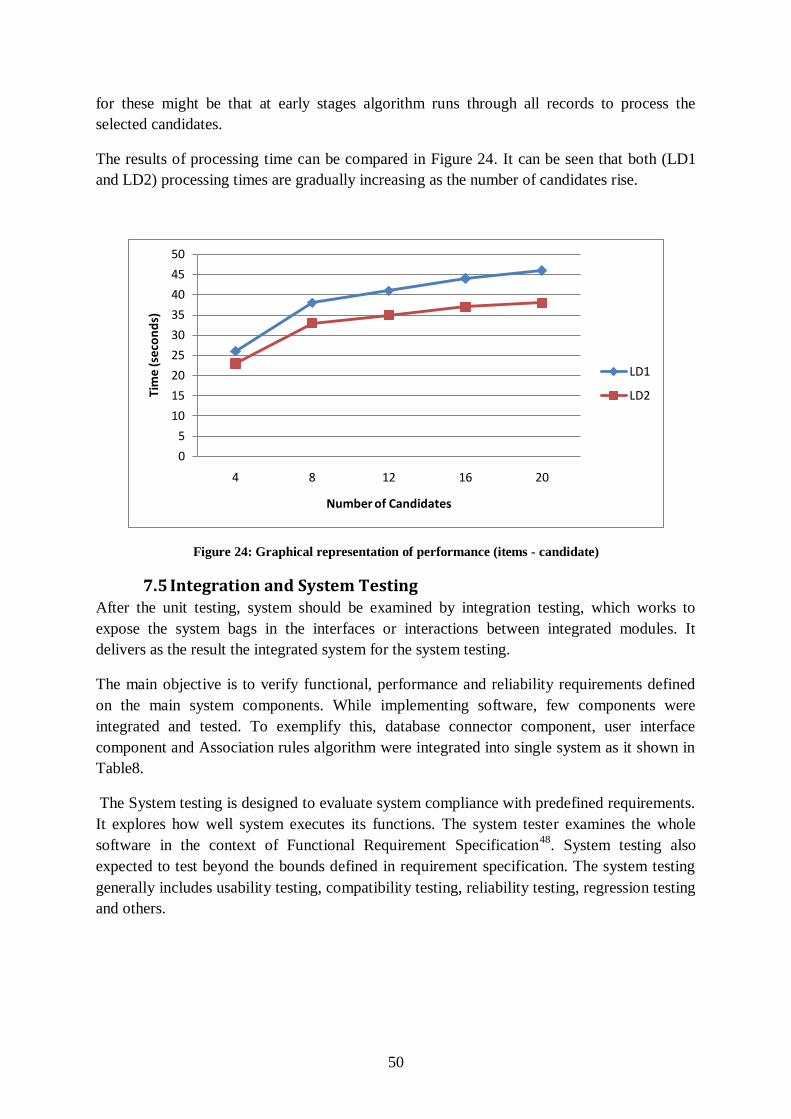
50

for these might be that at early stages algorithm runs through all records to process the

selected candidates.

The results of processing time can be compared in Figure 24. It can be seen that both (LD1

and LD2) processing times are gradually increasing as the number of candidates rise.

Figure 24: Graphical representation of performance (items - candidate)

7.5 Integration and System Testing After the unit testing, system should be examined by integration testing, which works to

expose the system bags in the interfaces or interactions between integrated modules. It

delivers as the result the integrated system for the system testing.

The main objective is to verify functional, performance and reliability requirements defined

on the main system components. While implementing software, few components were

integrated and tested. To exemplify this, database connector component, user interface

component and Association rules algorithm were integrated into single system as it shown in

Table8.

The System testing is designed to evaluate system compliance with predefined requirements.

It explores how well system executes its functions. The system tester examines the whole

software in the context of Functional Requirement Specification48

. System testing also

expected to test beyond the bounds defined in requirement specification. The system testing

generally includes usability testing, compatibility testing, reliability testing, regression testing

and others.

0

5

10

15

20

25

30

35

40

45

50

4 8 12 16 20

Tim

e (

seco

nd

s)

Number of Candidates

LD1

LD2

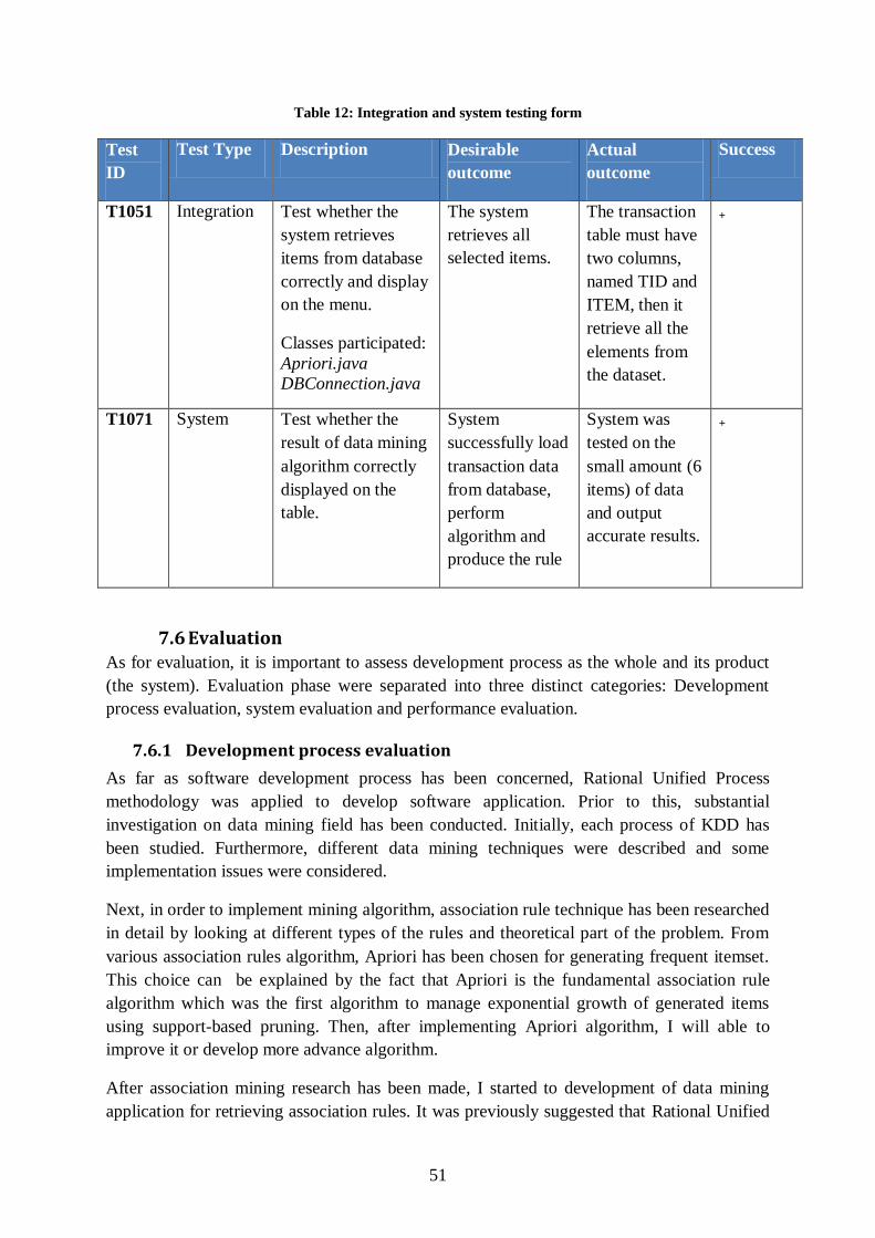
51

Table 12: Integration and system testing form

Test

ID

Test Type Description Desirable

outcome

Actual

outcome

Success

T1051 Integration Test whether the

system retrieves

items from database

correctly and display

on the menu.

Classes participated:

Apriori.java

DBConnection.java

The system

retrieves all

selected items.

The transaction

table must have

two columns,

named TID and

ITEM, then it

retrieve all the

elements from

the dataset.

+

T1071 System Test whether the

result of data mining

algorithm correctly

displayed on the

table.

System

successfully load

transaction data

from database,

perform

algorithm and

produce the rule

System was

tested on the

small amount (6

items) of data

and output

accurate results.

+

7.6 Evaluation As for evaluation, it is important to assess development process as the whole and its product

(the system). Evaluation phase were separated into three distinct categories: Development

process evaluation, system evaluation and performance evaluation.

7.6.1 Development process evaluation

As far as software development process has been concerned, Rational Unified Process

methodology was applied to develop software application. Prior to this, substantial

investigation on data mining field has been conducted. Initially, each process of KDD has

been studied. Furthermore, different data mining techniques were described and some

implementation issues were considered.

Next, in order to implement mining algorithm, association rule technique has been researched

in detail by looking at different types of the rules and theoretical part of the problem. From

various association rules algorithm, Apriori has been chosen for generating frequent itemset.

This choice can be explained by the fact that Apriori is the fundamental association rule

algorithm which was the first algorithm to manage exponential growth of generated items

using support-based pruning. Then, after implementing Apriori algorithm, I will able to

improve it or develop more advance algorithm.

After association mining research has been made, I started to development of data mining

application for retrieving association rules. It was previously suggested that Rational Unified

52

Process has been chosen, due to its flexibility and iterative approach. At early stages,

requirements were captured and system structure was outlines.

Next, system’s structure and behavior diagram were drawn and system prototype was

developed. After defining the system context, implementation technology was chosen and

coding process started. Finally, the system components were tested and evaluated. During

each iteration, system requirements, design and implementation decision were reviewed and

refined.

7.6.2 System evaluation

Regarding the system evaluation, software can be defined as successful if it satisfies all user

requirements. Data mining application has all essential features to process association rules

analysis. The main functionality, such as loading dataset from database, Association rule

algorithm mining, displaying and writing results have been developed. Furthermore,

additional features such as comparing and filtering results have been implemented.

For software implementation, Java was used, because it is object-oriented, platform

independent and simple language to use. For DBMS, MYSQL were used, because it is fast,

robust and with good feature set. For transaction operation, SQL was used due to its

performance and reliability. Furthermore, the combination of these tools is ideal for

development, because I have great experience on each of them. Finally, the implemented

system meets all critical requirements.

7.6.3 Performance evaluation

With respect to the performance of the application, in testing stage the performance has been

calculated. Two testing approach has been applied: support-related test and candidate-related

test. The former were calculating using different min support values on the same number of

candidate. The latter were processed different number of candidates but on the same support

threshold.

From the table 8 and 9, the findings of the experiments suggest that data mining application

works very quick on small and medium databases. In contrast, the speed of data mining

application on large dataset is noticeably slower. The main reason is that large dataset has

more items, which in their turn make bigger transaction width. Therefore, the algorithm will

spend more time scanning candidates, because more items were located in the same

transaction id. Overall, the performance of the application is good.

7.7 Summary In this section various testing techniques have been discussed. They help to identify the

correctness, completeness, quality and efficiency of developed data mining software. Finally

the software has been evaluated and feedbacks were provided.

53

Chapter 7: Conclusion

7.1 Overview This chapter describes what challenges were encountered and the set of desired features and

improvements could be implemented. Finally, personal opinion and recommendations of the

author are provided.

7.2 Personal Experience This paper describes the process of development data mining software application and

research made in corresponding .The subject of association rules discovery has been selected

due to the fact that the data mining software products are applied in different areas, including

business, science and medicine. The application can uncover previously unknown, hidden

and potentially useful information from the data. Personally, it was very interesting to

develop such software and see what results it can produce from the raw data. Especially in

our time, these kinds of applications are in demand as large amount of data collected from

various source, such as industry and internet.

Although the software development was not easy, it was very fascinating process for me. I

enjoyed by overcoming complex issues and taking decisions throughout the project. The

project helped me to gain academic knowledge as well as practical skills. I have learnt

fundamentals of association rule discovery and become specialist in data mining field. This

knowledge will certainly be useful in my future studies in Information Systems. Also, my

coding skills in Java have been improved as I have learnt new techniques and algorithms.

Personally, I have achieved great results in personal development, including time-

management, decision making and learning skills.

The main lesson learnt from the development process that in reality it is very challenging to

deliver a complete product in limited time. Even the most specifications were satisfied there

are always some things could be done to improve the system. Overall, the project was

successful as all compulsory requirements were met. Finally, the third year project was

unique and valuable experience for my future career.

7.3 Challenges Although the essential goal has been fulfilled, there were number of challenges to deal with.

The purpose of the project was to create software product which deals with huge datasets.

The main challenge of this data mining field is to efficiently process the large quantities of

data. Inefficient implementation of application may result on exponential computational

complexity of algorithm, which will require an exponentially increasing amount of resources,

such as processing time, computer memory. Therefore, I have chosen Apriori algorithm,

which deals with exponential growth of generated items. I repeatedly tested the application

using sample dataset, to ensure the correctness and effectiveness of my program.

Another issue was choosing right data structure for storing and processing frequent itemsets

from databases. At the beginning, I planned to create my own data structure. However, after

54

studying existed implementation, I decided to use Hash Map and ArrayList from the Java

API, because of their high-quality implementation and high-performance.

Next problem was running multiple algorithms simultaneously, without effect on

performance. It was partially resolved using concurrency support provided by Java platform.

7.4 Further Improvements As for desired improvements, there are number features which could be implemented if more

time was available. There were many data mining techniques to choose from, whereas I

selected Association rule Discovery, due to my interest in this area. Perhaps, I could research

other mining methodologies (e.g., clustering, classification and regression), if more time

would be available. However I did briefly studied and described them in the second chapter,

so this research helped to make my choice in favor of association rules.

In chapter 3, I have described about other types of Association Algorithm: Generalized,

Quantitative, Categorical and Temporal Association rule. Therefore, the software could

support more sophisticated properties of data such as time, quantity, category and other

attributes of data. If I had more time, I would explore more advanced implementation of

association rules looking at various methods for generating frequent item set. The possible

options could include FP-growth algorithm, ECLAT and Apriori-TID. As the result, the

mining processing could be more efficient and would require less processing time.

Furthermore, I would also like to look at more complex algorithm feature, multiple support

measure and negative support value etc. Thus, mining results would offer more precise and

“more interesting” rules to data analytics, by eliminating trivial, irrelevant and misleading

results. Then, interpretation and evaluation stage would be simplified and quickly conducted.

As for extra functionality of the developed system, there several features, which I would like

to improve or add to the system. First of all, the system would process all stages of

Knowledge Discovery Process, from data selection/preprocessing to data evaluation phase.

The data analytics would process all cycles of KDD using only this software. Secondly, the

system also would be developed to read “raw data” from different data sources (CSV, Ms

Excel, XML etc.) of and export results into various data formats (databases, Ms Excel or

Web). The system would be more flexible and may ease some pre/post processing work.

Additionally, as the part of KDD process, association rules could be visualized as two or

three dimensional graph to make easier for analytics to investigate the results. As an

alternative, the table with the results has been implemented by highlighting some interesting

rules. Next, I have considered, that it is better to create my own data structure for storing item

sets, if I could develop my project from scratch. It will bring more flexibility and greater

control over the data. Also, I would choose the C++, because it has higher performance.

Finally, it would be better if system could operate on the web, so there will be two versions:

online and desktop application.

55

References 1 Dr. Osmar R. Zaiane, (1999) “Introduction to data mining” [online] Available

from:<http://webdocs.cs.ualberta.ca/~zaiane/courses/cmput690/slides/Chapter1/sld011.htm> [cited 25/02/10]

2 Kenneth Cukier, (2010) “Data, data everywhere”, The Economist, pp 1-3, a special report on managing

information, Feb 27. 3 Kenneth Cukier, (2010) “Data, data everywhere”, The Economist, pp 3-4, A special report on managing

information, Feb 27.

4 Kenneth Cukier, (2010) “All too much”, The Economist, pp 3, A special report on managing information,

Feb 27.

5 Karl Rexeter (2009) “2009 Data Miner Survey” [online] Available from: <

http://www.rexeranalytics.com/Data-Miner-Survey-Results-2009.html> [cited 28/04/10]

6 Karl Rexeter (2007) “2007 KDD Nuggets Survey” [online] Available from: <http://www.the-data-

mine.com/bin/view/Software/MostPopularDataMiningSoftware> [cited 28/04/10]

7 “Project details for WEKA” (2010) [online] Available from:

<http://mloss.org/media/screenshot_archive/weka_explorer_screenshot.png> [cited 28/04/10]

8 Wikipedia (2010) "WEKA (machine learning)” [online] Available from:

<http://en.wikipedia.org/wiki/Weka_(machine_learning)> [cited 28/04/10]

9 Wikipedia (2010), “Data mining” [online] Available from: <http://en.wikipedia.org/wiki/Data_mining> [cited

28/04/10]

10 U. Fayad, G. Piatetsky-Shpiro, P. Smyth (1996) From data mining to knowledge discovery: An overview. In

Advances in Knowledge Discovery and Data Mining, AAAI/MIT Press, Cambridge.

11 Rithm (2010), “Knowledge discovery in database” [online] Available from: <

http://www.rithme.eu/?m=home&p=kdprocess&lang=en> [cited 28/04/10]

12 U. Fayad, G. Piatetsky-Shpiro, P. Smyth (1996) “The KDD Process for Extracting Useful Knowledge from Volumes of Data”, Communication of the ACM; Vol. 39, No. 11 13 Cross Industry Standard Process for Data Mining (2010) “About CRISP-DM” [online] Available from: <

http://www.crisp-dm.org/> [cited 28/04/10]

14 M.F. Hornick, E. Marcade, S. Venkayala, (2007) “Java Data Mining: Strategy, Standard, and Practice”;

Elsevier Inc. pp 52-59

15 Aerlingus.com (2010) “AerLingus systems” [online] Available from: <

http://student.dcu.ie/~czakanm2/ca596/asgn2datamining.html>

16 Dr. Osmar R. Zaiane, (1999) “Principles of Knowledge Discovery in Databases” [online] Available from:

<http://webdocs.cs.ualberta.ca/~zaiane/courses/cmput690/ > [cited 28/04/10]

17 Mike Chapple, About.com (2010), “Regression”, [online] Available from: <

http://databases.about.com/od/datamining/g/regression.htm>

18 Wikipedia (2010), "Cluster Analysis” [online] Available from: <

http://en.wikipedia.org/wiki/Cluster_analysis> [cited 28/04/10]

19 MSDN, (2010) “Data Mining Algorithm” [online] Available from: < http://msdn.microsoft.com/en-

us/library/ms175595.aspx> [cited 28/04/10]

http://webdocs.cs.ualberta.ca/~zaiane/courses/cmput690/slides/Chapter1/sld011.htm

http://www.rexeranalytics.com/Data-Miner-Survey-Results-2009.html

http://www.the-data-mine.com/bin/view/Software/MostPopularDataMiningSoftware

http://www.the-data-mine.com/bin/view/Software/MostPopularDataMiningSoftware

http://mloss.org/media/screenshot_archive/weka_explorer_screenshot.png

http://en.wikipedia.org/wiki/Weka_(machine_learning)

http://en.wikipedia.org/wiki/Data_mining

http://www.rithme.eu/?m=home&p=kdprocess&lang=en

http://www.crisp-dm.org/

http://student.dcu.ie/~czakanm2/ca596/asgn2datamining.html

http://webdocs.cs.ualberta.ca/~zaiane/courses/cmput690/slides/Chapter1/sld011.htm

http://databases.about.com/od/datamining/g/regression.htm

http://en.wikipedia.org/wiki/Cluster_analysis

http://msdn.microsoft.com/en-us/library/ms175595.aspx

http://msdn.microsoft.com/en-us/library/ms175595.aspx

56

20 Wikipedia (2010), "Association rule learning” [online] Available from: <

http://en.wikipedia.org/wiki/Association_rule_learning [cited 28/04/10]

21 M.H. Dunham (2003) “Data Mining: Introduction and advance topics” Pearson Education, Inc. pp 8.

22 M.H. Dunham (2003) “Data Mining: Introduction and advance topics” Pearson Education, Inc. pp 14-15.

23 Wikipedia (2010), "Association rule learning” [online] Available from: <

http://en.wikipedia.org/wiki/Association_rule_learning> [cited 28/04/10]

24 P. Tan, M. Steinbach, V, Kumar (2006) “Introduction to data mining” Pearson Education, Inc. pp 327.

25 P. Tan, M. Steinbach, V, Kumar (2006) “Introduction to data mining” Pearson Education, Inc. pp 328-330

26 P. Tan, M. Steinbach, V, Kumar (2006) “Introduction to data mining” Pearson Education, Inc. pp 374

27 J, Han, M. Kamber (2001) “Data Mining: Concept and Technique” Academic Press, San Diego pp 228


29 P. Tan, M. Steinbach, V, Kumar (2006) “Introduction to data mining” Pearson Education, Inc. pp 337-352

30 M.H. Dunham (2003) “Data Mining: Introduction and advance topics” Pearson Education, Inc. pp 236-238

31 M.H. Dunham (2003) “Data Mining: Introduction and advance topics” Pearson Education, Inc. pp 184-186

32 Ilias Patrounias, Xiaodong Chen, Discovering Temporal Association Rules: Algorithm, Language and System

(2000) [online] Available from: < http://www.computer.org/portal/web/csdl/doi/10.1109/ICDE.2000.839423>

[cited 28/04/10]

33 Y. Kambayashi, Mukesh Mohania, A Min Tjoa (2001) Second International Conference on Data

Warehousing and Knowledge Discovery, pp 329, Springer(London)

34 Y. Kambayashi, Mukesh Mohania, A Min Tjoa (2001) Second International Conference on Data

Warehousing and Knowledge Discovery, pp 330, Springer(London)


36 G. Larman (2005) “Appling UML and Patterns” Pearson Education, Inc pp 18.

37 Openia, (2010) Methodology, [online] Available from: < http://www2.openia.com/about/methodology>

[cited 28/04/10]

38 SearchSoftwareQuality (2007) “requirements analysis”, [online] Available from: <

http://searchsoftwarequality.techtarget.com/sDefinition/0,,sid92_gci1248686,00.html> [cited 28/04/10]

39 Dr Siobhan Devlin (2010) ”requirement analysis and definition”, [online] Available from: <

http://osiris.sunderland.ac.uk/~cs0sdv/CSE100/> [cited 28/04/10]

40 Lesson from History (2009) “Functional versus Non-Functional Requirements and Testing” [online]

Available from: < http://www.lessons-from-history.com/node/83>[cited 28/04/10]

41 Ruth Malan and Dana Bredemeyer (2010) “Functional Requirements and Use Cases” [online] Available

from: < https://docs.google.com/viewer?url=http://www.bredemeyer.com/pdf_files/functreq.pdf> [cited

28/04/10]

http://en.wikipedia.org/wiki/Association_rule_learning

http://en.wikipedia.org/wiki/Association_rule_learning

http://www.computer.org/portal/web/csdl/doi/10.1109/ICDE.2000.839423

http://www2.openia.com/about/methodology

http://searchsoftwarequality.techtarget.com/sDefinition/0,,sid92_gci1248686,00.html

http://osiris.sunderland.ac.uk/~cs0sdv/CSE100/

http://www.lessons-from-history.com/node/83

https://docs.google.com/viewer?url=http://www.bredemeyer.com/pdf_files/functreq.pdf

57

42 Jakob Nielsen (2010) “Ten Usability Heuristics” [online] Available from: < 43 Eric Lain (2008) “ComputerWorld” [online] Available from:

<http://www.computerworld.com/s/article/9087918/Size_matters_Yahoo_claims_2_petabyte_database_is_worl

d_s_biggest_busiest>[cited 28/04/10]

44 YookStore (2010) “Why SQL?” [online] Available from: <http://www.yook.com/sql/>[cited 28/04/10]

45 J, Han, M. Kamber (2001) “Data Mining: Concept and Technique” Academic Press, San Diego pp 235

46 The Java Tutorials (2010) “Buffered streams” [online] Available from:

<http://java.sun.com/docs/books/tutorial/essential/io/buffers.html>[cited 28/04/10]

47 MySQL Forge (2010) “Spawner Data Generator” [online] Available from: <

http://forge.mysql.com/projects/project.php?id=214>[cited 28/04/10]

48 Wikipedia (2010), "System Testing” [online] Available from: < http://en.wikipedia.org/wiki/System_testing>

[cited 28/04/10]

http://www.useit.com/jakob/

http://www.computerworld.com/s/article/9087918/Size_matters_Yahoo_claims_2_petabyte_database_is_world_s_biggest_busiest

http://www.computerworld.com/s/article/9087918/Size_matters_Yahoo_claims_2_petabyte_database_is_world_s_biggest_busiest

http://www.yook.com/sql/

http://java.sun.com/docs/books/tutorial/essential/io/buffers.html

http://forge.mysql.com/projects/project.php?id=214

http://en.wikipedia.org/wiki/System_testing

zhanat zhanibekov - university of...

Documents