zero to matlab - classes

Zero to MATLAB

Adam L. Lambert, PhD

January 7, 2019

Contents

1 Introduction 7

2 The Basics 92.1 Calculations with Operators. . . . . . . . . . . . . . . . . . . . . . . . . . . . . . . . . . . 11

2.1.1 Order of Operations . . . . . . . . . . . . . . . . . . . . . . . . . . . . . . . . . . . 122.1.2 Matching Parentheses . . . . . . . . . . . . . . . . . . . . . . . . . . . . . . . . . . 132.1.3 Practice . . . . . . . . . . . . . . . . . . . . . . . . . . . . . . . . . . . . . . . . . 13

2.2 Calculations with Functions. . . . . . . . . . . . . . . . . . . . . . . . . . . . . . . . . . . 142.2.1 Trigonometry . . . . . . . . . . . . . . . . . . . . . . . . . . . . . . . . . . . . . . 142.2.2 Square Root . . . . . . . . . . . . . . . . . . . . . . . . . . . . . . . . . . . . . . . 152.2.3 Rounding . . . . . . . . . . . . . . . . . . . . . . . . . . . . . . . . . . . . . . . . 15

2.3 Documentation . . . . . . . . . . . . . . . . . . . . . . . . . . . . . . . . . . . . . . . . . 152.4 Calculations with Variables. . . . . . . . . . . . . . . . . . . . . . . . . . . . . . . . . . . . 16

2.4.1 Deleting Variables . . . . . . . . . . . . . . . . . . . . . . . . . . . . . . . . . . . . 182.4.2 Naming Variables . . . . . . . . . . . . . . . . . . . . . . . . . . . . . . . . . . . . 182.4.3 Assignment Operator . . . . . . . . . . . . . . . . . . . . . . . . . . . . . . . . . . 192.4.4 Semicolon . . . . . . . . . . . . . . . . . . . . . . . . . . . . . . . . . . . . . . . . 19

2.5 Scripting . . . . . . . . . . . . . . . . . . . . . . . . . . . . . . . . . . . . . . . . . . . . . 202.5.1 m-files . . . . . . . . . . . . . . . . . . . . . . . . . . . . . . . . . . . . . . . . . . 202.5.2 Text Editor . . . . . . . . . . . . . . . . . . . . . . . . . . . . . . . . . . . . . . . 202.5.3 Problem Solving with Scripts . . . . . . . . . . . . . . . . . . . . . . . . . . . . . . 23

2.6 Input/Output . . . . . . . . . . . . . . . . . . . . . . . . . . . . . . . . . . . . . . . . . . 252.6.1 input . . . . . . . . . . . . . . . . . . . . . . . . . . . . . . . . . . . . . . . . . . 262.6.2 disp . . . . . . . . . . . . . . . . . . . . . . . . . . . . . . . . . . . . . . . . . . . 26

2.7 Errors . . . . . . . . . . . . . . . . . . . . . . . . . . . . . . . . . . . . . . . . . . . . . . 262.8 Exercises . . . . . . . . . . . . . . . . . . . . . . . . . . . . . . . . . . . . . . . . . . . . . 28

3 Algorithms I 313.1 Manual Plotting . . . . . . . . . . . . . . . . . . . . . . . . . . . . . . . . . . . . . . . . . 313.2 Organization . . . . . . . . . . . . . . . . . . . . . . . . . . . . . . . . . . . . . . . . . . . 333.3 Conical Tank . . . . . . . . . . . . . . . . . . . . . . . . . . . . . . . . . . . . . . . . . . . 34

4 Looping and Plotting 394.1 The for-loop . . . . . . . . . . . . . . . . . . . . . . . . . . . . . . . . . . . . . . . . . . 394.2 Row Arrays . . . . . . . . . . . . . . . . . . . . . . . . . . . . . . . . . . . . . . . . . . . 404.3 Indexing . . . . . . . . . . . . . . . . . . . . . . . . . . . . . . . . . . . . . . . . . . . . . 424.4 Plotting with Indexing. . . . . . . . . . . . . . . . . . . . . . . . . . . . . . . . . . . . . . 424.5 The Colon Operator . . . . . . . . . . . . . . . . . . . . . . . . . . . . . . . . . . . . . . . 444.6 Indexing with Variables . . . . . . . . . . . . . . . . . . . . . . . . . . . . . . . . . . . . . 454.7 Plotting with the for-loop. . . . . . . . . . . . . . . . . . . . . . . . . . . . . . . . . . . . 474.8 Counting with the for-loop . . . . . . . . . . . . . . . . . . . . . . . . . . . . . . . . . . . 494.9 Exponential Decay. . . . . . . . . . . . . . . . . . . . . . . . . . . . . . . . . . . . . . . . 504.10 Adaptive Looping . . . . . . . . . . . . . . . . . . . . . . . . . . . . . . . . . . . . . . . . 514.11 Plot Formatting . . . . . . . . . . . . . . . . . . . . . . . . . . . . . . . . . . . . . . . . . 544.12 Naming Index Variables . . . . . . . . . . . . . . . . . . . . . . . . . . . . . . . . . . . . . 564.13 Index Dimension Errors . . . . . . . . . . . . . . . . . . . . . . . . . . . . . . . . . . . . . 56

3

Contents

4.14 Exercises . . . . . . . . . . . . . . . . . . . . . . . . . . . . . . . . . . . . . . . . . . . . . 57

5 Logical Operations 615.1 Relational Operators . . . . . . . . . . . . . . . . . . . . . . . . . . . . . . . . . . . . . . . 61

5.2 if-statements. . . . . . . . . . . . . . . . . . . . . . . . . . . . . . . . . . . . . . . . . . . 62

5.3 Looping with if-statements. . . . . . . . . . . . . . . . . . . . . . . . . . . . . . . . . . . 63

5.4 if-else-statements. . . . . . . . . . . . . . . . . . . . . . . . . . . . . . . . . . . . . . . 67

5.5 if-elseif-else-statements . . . . . . . . . . . . . . . . . . . . . . . . . . . . . . . . . 67

5.6 Testing Data . . . . . . . . . . . . . . . . . . . . . . . . . . . . . . . . . . . . . . . . . . . 68

5.7 Boolean Operations . . . . . . . . . . . . . . . . . . . . . . . . . . . . . . . . . . . . . . . 69

5.8 Errors & Troubleshooting . . . . . . . . . . . . . . . . . . . . . . . . . . . . . . . . . . . . 72

5.9 Exercises . . . . . . . . . . . . . . . . . . . . . . . . . . . . . . . . . . . . . . . . . . . . . 73

6 Nested Loops 756.1 Indexing in Two Dimensions. . . . . . . . . . . . . . . . . . . . . . . . . . . . . . . . . . . 75

6.2 Nested for-loops . . . . . . . . . . . . . . . . . . . . . . . . . . . . . . . . . . . . . . . . 76

6.2.1 Counting With Nested Loops . . . . . . . . . . . . . . . . . . . . . . . . . . . . . . 77

6.2.2 Nested Wavenumbers . . . . . . . . . . . . . . . . . . . . . . . . . . . . . . . . . . 78

6.3 Ideal Gas Law Isotherms . . . . . . . . . . . . . . . . . . . . . . . . . . . . . . . . . . . . . 79

6.4 Plotting in 3D. . . . . . . . . . . . . . . . . . . . . . . . . . . . . . . . . . . . . . . . . . . 81

6.5 Nested Sums. . . . . . . . . . . . . . . . . . . . . . . . . . . . . . . . . . . . . . . . . . . 82

6.6 Exercises . . . . . . . . . . . . . . . . . . . . . . . . . . . . . . . . . . . . . . . . . . . . . 84

7 Formatted Output 857.1 Strings . . . . . . . . . . . . . . . . . . . . . . . . . . . . . . . . . . . . . . . . . . . . . . 85

7.1.1 Concatenation . . . . . . . . . . . . . . . . . . . . . . . . . . . . . . . . . . . . . . 85

7.1.2 num2str . . . . . . . . . . . . . . . . . . . . . . . . . . . . . . . . . . . . . . . . . 86

7.1.3 strcmp . . . . . . . . . . . . . . . . . . . . . . . . . . . . . . . . . . . . . . . . . 87

7.2 fprintf . . . . . . . . . . . . . . . . . . . . . . . . . . . . . . . . . . . . . . . . . . . . . 87

7.2.1 Basic Formatting . . . . . . . . . . . . . . . . . . . . . . . . . . . . . . . . . . . . 87

7.2.2 Special Characters . . . . . . . . . . . . . . . . . . . . . . . . . . . . . . . . . . . . 89

7.2.3 Multiple Input Variables . . . . . . . . . . . . . . . . . . . . . . . . . . . . . . . . . 89

7.2.4 Aesthetics . . . . . . . . . . . . . . . . . . . . . . . . . . . . . . . . . . . . . . . . 90

7.2.5 Printing to Files . . . . . . . . . . . . . . . . . . . . . . . . . . . . . . . . . . . . . 90

7.3 Exercises . . . . . . . . . . . . . . . . . . . . . . . . . . . . . . . . . . . . . . . . . . . . . 91

8 Functions 938.1 Basic Functions . . . . . . . . . . . . . . . . . . . . . . . . . . . . . . . . . . . . . . . . . 93

8.2 Function Workspace . . . . . . . . . . . . . . . . . . . . . . . . . . . . . . . . . . . . . . . 95

8.3 Practical Functions . . . . . . . . . . . . . . . . . . . . . . . . . . . . . . . . . . . . . . . 96

8.4 Errors . . . . . . . . . . . . . . . . . . . . . . . . . . . . . . . . . . . . . . . . . . . . . . 98

8.5 Cody . . . . . . . . . . . . . . . . . . . . . . . . . . . . . . . . . . . . . . . . . . . . . . . 99

8.6 Exercises . . . . . . . . . . . . . . . . . . . . . . . . . . . . . . . . . . . . . . . . . . . . . 99

9 Algorithms II 1019.1 Coin Flip . . . . . . . . . . . . . . . . . . . . . . . . . . . . . . . . . . . . . . . . . . . . . 101

9.1.1 Fairness . . . . . . . . . . . . . . . . . . . . . . . . . . . . . . . . . . . . . . . . . 102

9.1.2 Counting Streaks . . . . . . . . . . . . . . . . . . . . . . . . . . . . . . . . . . . . 103

9.2 Exercises . . . . . . . . . . . . . . . . . . . . . . . . . . . . . . . . . . . . . . . . . . . . . 107

10 Array Operations 10910.1 Simple Array Operations . . . . . . . . . . . . . . . . . . . . . . . . . . . . . . . . . . . . 109

10.2 Matrix Operations . . . . . . . . . . . . . . . . . . . . . . . . . . . . . . . . . . . . . . . . 110

10.3 The “dot” Operator . . . . . . . . . . . . . . . . . . . . . . . . . . . . . . . . . . . . . . . 110

10.4 Implicit Expansion . . . . . . . . . . . . . . . . . . . . . . . . . . . . . . . . . . . . . . . . 111

4

Contents

10.5 Logical Indexing . . . . . . . . . . . . . . . . . . . . . . . . . . . . . . . . . . . . . . . . . 111

11 Data Processing 11311.1 Basic Statistics . . . . . . . . . . . . . . . . . . . . . . . . . . . . . . . . . . . . . . . . . 11311.2 Fitting Data . . . . . . . . . . . . . . . . . . . . . . . . . . . . . . . . . . . . . . . . . . . 11311.3 Nonlinear Data . . . . . . . . . . . . . . . . . . . . . . . . . . . . . . . . . . . . . . . . . 115

12 Data Structures 11712.1 Tables . . . . . . . . . . . . . . . . . . . . . . . . . . . . . . . . . . . . . . . . . . . . . . 11712.2 Structs . . . . . . . . . . . . . . . . . . . . . . . . . . . . . . . . . . . . . . . . . . . . . . 11912.3 Cell Arrays . . . . . . . . . . . . . . . . . . . . . . . . . . . . . . . . . . . . . . . . . . . . 120

13 ODE Solvers 12313.1 ode45 . . . . . . . . . . . . . . . . . . . . . . . . . . . . . . . . . . . . . . . . . . . . . . 12313.2 ode15s . . . . . . . . . . . . . . . . . . . . . . . . . . . . . . . . . . . . . . . . . . . . . . 125

Index 127

5

1 Introduction

The MATLAB programming language is commonly used in engineering and scientific computation. I wrotethis book to give first year students a basic introduction to MATLAB syntax and algorithmic thinking. Thisis by no means a comprehensive resource. It is meant to get students started and allow them to transitionto more complex material.

The book is structured as a tutorial rather than a reference. The MATLAB documentation is extensiveand so my focus will be to outline basic algorithmic thinking and MATLAB syntax with explicit examples. Iencourage students to work through the chapters in order as each new concept builds on previous material.

The initial chapters require only basic algebra and geometry, so they are accessible to students at any pointin their math sequence. Many of the problems in these chapters will seem simple or tedious. They are. Thepurpose is to separate the skill that you wish to develop (MATLAB programming) from other skills whichneed to be developed. The simple problems allow you to focus on the hard work of communicating with thecomputer. Once you’re comfortable with that, then you try to apply algorithmic thinking to more interestingproblems.

Later chapters demonstrate some more advanced features in simple, accessible examples.

7

2 The Basics

Before we dive into algorithms and problem solving, we need to gain some basic familiarity with MATLAB.In this chapter we’ll explore the Graphical User Interface (GUI) and learn how to use MATLAB for simplecalculations. In the last section, we’ll learn how to save a series of MATLAB commands in a file and executethem as a single program. At the end you will find some exercises to test your learning.

Installing MATLAB

The installation is well documented and straightforward so I will not cover it in detail. If you have a universitylicense that includes many of the toolboxes, we will only be using the basic installation. They might beuseful later on in your education, but for now you can save the space on your hard drive.

Launching MATLAB

If you are on a Windows computer then you can launch MATLAB from your Start menu. It will also giveyou the option to make a desktop icon during installation. On a Mac, you should be able to find it in yourapplications folder.

Depending on your computer it may take some time to load. Eventually a window will open, shown in Figure2.1.

Figure 2.1: MATLAB GUI

9

2 The Basics

Interface

Generally speaking there are two methods for interacting directly with software. A Text Based Interface(TUI) requires the user to type in commands in order to initiate an action. A Graphical User Interface(GUI) allows a user to interact with the software through images, icons, and readable menus. Most modernsoftware utilizes a GUI. The majority of our interactions with MATLAB will be text based, but the GUIprovides several nice features which make the process of computer programming much simpler.

MATLAB offers an interactive Command Window for executing individual commands. This is very conve-nient, because otherwise we would have to execute a compiler or interpreter every single time we wanted toperform a basic calculation or test a command. By default, the Command Window is located in the middleof the MATLAB GUI. It is labeled at the top as “Command Window” and contains a prompt in the upperleft which looks like this:

>>

We can use the Command Window to perform basic calculations. Expressions are entered at the prompt,when completed the user can execute the expression using Enter .

Figure 2.2: Calculations are typed directly into the Command Window at the prompt.

MATLAB will perform the calculation and report the answer directly in the Command Window as shownin Figure 2.3. Don’t worry about the ans variable name for now. We’ll learn all about it later in thechapter when we discuss variables. In the next section, we’ll learn about basic MATLAB syntax and orderof operations.

10

2.1 Calculations with Operators.

Figure 2.3: MATLAB returns the results in the Command Window by default.


I’m going to dive into some mathematical detail in this section. The details are important because ultimatelycomputational tools are tools for doing math. Please don’t skip over the discussion about addition andsubtraction just because you learned how to do them in elementary school. I promise that the discussion isrelevant to your understanding.

When we perform a calculation like addition, we are performing a mathematical operation. That is, we usea mathematical operator to combine two numbers into a sum. It’s a nebulous concept that most of us takefor granted every day, but as we dive into computational problem solving, the details get very important.

The general definition of a mathematical operator can be interpreted as “a mapping that acts on theelements of a space to produce other elements of the same space.” In the case of adding two real numbers,the addition operator is the mapping and the two real numbers are the elements. The result is anotherreal number which represents the sum, or total, of the two elements. Don’t get to hung up on the word“mapping.” Just understand that the mathematical operation is the thing that you do when you perform abasic calculation.

Addition, subtraction, multiplication, division, and exponentiation are all operations and the symbol asso-ciated with each of them is an operator. MATLAB syntax for the common algebraic operators is given inTable 2.1.

Table 2.1: Operator Syntax

Expression MATLAB Command

a+ b a+b

a− b a-b

a ∗ b a*bab a/b

a2 aˆ2

We already learned that we can enter basic calculations right in the Command Window. Go ahead and typethe following expression at the prompt and press Enter .

>>3+5

11

2 The Basics

In this case, MATLAB will apply the addition operator to the numbers 3 and 5 and then report the result.Try out the other operators with these examples.

>>12-5

>>7/5

>>2*5

MATLAB doesn’t care about white spaces, so if you prefer to space out the calculations for readability thenthat’s fine. The commands below will return the same as the ones we just tried.

>> 12 - 5

>> 7 / 5

>> 2 * 5

2.1.1 Order of Operations

At some point you likely studied order of operations, the collection of rules for the order in which we performmathematical operations in complex expressions. Generally, MATLAB follows the familiar PEMDAS standardshown in Table 2.2.

Table 2.2: Hierarchy of operators.

Order Operation

1 Parentheses, Exponents2 Multiplication, Division3 Additions, Subtraction

However, within each level MATLAB interprets the expression from left to right. This results it somealgebraic expressions which must be written with parentheses in MATLAB. Consider the fraction:

7 + 18

11

Since we can only input a single line of text in the Command Window, a user might be tempted to inputthe expression:

>> 7+18/11

MATLAB will evaluate the division operation first, and then the addition, but fraction bars are groupingsymbols just like parenthesis so that expression would result in an incorrect answer. Instead, we need toforce the addition operation to go first by using parentheses like this:

>> (7+18)/11

You can read more about operator precedence in the MATLAB documentation here:https://www.mathworks.com/help/matlab/matlab_prog/operator-precedence.html

12

https://www.mathworks.com/help/matlab/matlab_prog/operator-precedence.html


2.1.2 Matching Parentheses

As expressions become more complex, additional parentheses are required. It can be difficult to determinewhich particular left and right parenthesis actually line up. Fortunately there is a feature in MATLAB tohelp with this problem. It’s difficult to show in a picture, but if you work through the example below itshould be clear.

1. Type this expression in the Command Window and do not press a key. Leave your cursor blinking atthe end of the expression.

>>2*(3 + 5)

2. Now, use the left and right arrow keys ( , ) to move the cursor back and forth over the lastparenthesis.

3. Notice the brief underline that appears under each of the parentheses as you move the cursor. Thatunderline is indicating that those two parentheses match.

4. Lets make the expression more complex.

>>2*(3 + 5/(2+7))

5. Use the arrow keys to move the cursor and pay careful attention to how the corresponding parenthesisis underlined. This will be an important tool as we move into more complex expressions, so I encourageyou to make sure you understand how to correctly identify currently paired parentheses.

2.1.3 Practice

Let’s practice our new MATLAB syntax with some basic algebraic expressions. Pay careful attention to orderof operations. The answers are provided so that you can check your work.

1. 5.5− 4.1 [ans 1.4]

2. 5.7−2.84.3 [ans 0.6744]

3. (7.5−2.8∗0.87)4.3 [ans 1.177]

4. 7.5−2.84.32

[ans 0.2542]

5.(3∗2.2−2.8

4.3

)3+ 3 [ans 3.6902]

6.(422.1+7101.7

)2[ans 2.6304e+ 03]

Notice the format of the answer to expression #6. That format is generally referred to as engineeringnotation which is a form of scientific notation. The “e” stands for “×10n” where n is the number after thee. Here are two examples of numbers in both scientific and engineering format.

3.678× 106 = 3.678e+06

2.432× 10−4 = 2.432e-04

13

2 The Basics

Technically, proper engineering format requires that all exponents be multiples of 3 which helps the numberscale with SI unit prefixes. MATLAB does not implement that constraint, but simply uses the shorthand toprint the exponent in a readable format.

2.2 Calculations with Functions.

Just like the scientific calculator that you used in high school, MATLAB includes many common mathematicalfunctions. At this point I want to distinguish between a mathematical function and a programmatic function,otherwise known as a subroutine.

In mathematics, a function is a relation between a set of inputs and a set of permissible outputs with theproperty that each input is related to exactly one output. Basically, a function transforms a number or setof numbers, or perhaps even another function. For example, the cosine of an angle transforms the inputangle into the length of the x-projection as a fraction of the hypotenuse. There is only one possible resultfor any given angle.

A programmatic function is just a set of instructions that can be executed with an input. There are manyparallels between the two concepts, but a programmatic function does not have adhere to the mathematicaldefinition. We’ll learn how to build our own programmatic functions later in the book, but for now justunderstand that the mathematical functions we will study in this section are evaluated using programmaticfunctions which are included with MATLAB. We will call these included functions built-in functions.

TL;DR We heard you like functions so we put some functions in your functions.

There are many built-in functions in the MATLAB platform which will become useful as your educationprogresses. Once you get comfortable with the basic usage, it’s easy to read about new functions in thedocumentation. In this section we’ll cover some basic built-in functions which should be familiar to anyonewho has had algebra and trigonometry.

Most of these functions will appear in later examples, so take the time to familiarize yourself with the basicusage.

2.2.1 Trigonometry

The familiar trigonometric functions, sine, cosine, and tangent, are included in the platform as well as thevalue of π to several significant figures. The syntax for these functions is shown in Table 2.3.

Table 2.3: Trigonometric Functions

Expression MATLAB Syntax

sin(x) sin(x)

cos(x) cos(x)

tan(x) tan(x)

π pi

Note, the value of x must have units of radians! For more information, check out the MATLAB docu-mentation by typing doc sin, doc cos, or doc tan into the Command Window.

Let’s test the functions with some basic evaluations. Is the output what you expected?

14

2.3 Documentation

• sin(3.14)

• sin(π)

• sin(π2 )

• sin(π4 )

• cos(π)

• cos(π2 )

• cos(π4 )

• tan(3π4 )

You might have noticed that sin(π) and cos(π2 ) did not return zero, but instead a very small number inengineering notation. This is because MATLAB is doing a numerical approximation of these functions andcannot get exactly zero. However, for any reasonable engineering calculation, 10−16 is as close to zero aswe need to be.

2.2.2 Square Root

The square root function is given as:

Expression MATLAB Syntax√x sqrt(x)

Try the following expressions:

•√4 [ans 2]

•√9 [ans 3]

• 3+√2

7 [ans 0.6306]

• 2∗32.1+√2√

5+7[ans 2.3283]

2.2.3 Rounding

round(x): This function will round a number, x, to the nearest integer.

ceil(x): This function will round a number, x, up to the next integer.

floor(x): This function will round a number, x, down to the next integer.

Try each rounding function on the numbers 2.7 and 5.2.

2.3 Documentation

MATLAB installs documentation that you can access from the Command Window. This documentationexplains the usage of each built-in function. There are two commands for accessing the documentation,doc and help. In most cases you’ll want to use the doc command, since it opens an external window withrichly formatted text. The help command displays the information directly in the Command Window.

To use the doc command, just type the name of the function after like this.

15

2 The Basics

>>doc sin

2.4 Calculations with Variables.

In the previous sections we entered raw numbers into the Command Window, much like you would with ascientific calculator. You might have noticed that the output to your evaluations was preceded by some textthat read:

ans = ...

This is because MATLAB stores numbers as variables, and the default variable name is ans which is shortfor answer. We can define our own variable names, but first we should take the time to understand exactlywhat a variable is. The concept is very similar to what you have encountered in algebra, but there are somespecific differences which are important to your understanding of MATLAB.

MATLAB has to store values in the computer’s memory, and in order to find them again, there has to be aunique label which complies with MATLAB’s syntax. In the most basic terms, a variable is a combinationof value and label which allows us to store a number and perform an operation.

In MATLAB, the portion of the computer’s memory which used for variable storage is called the Workspace.At any time we can see the variables which are stored. In Figure 2.4, you can see my MATLAB GUI,including the Workspace, after I completed the previous exercises.

Figure 2.4: The MATLAB Workspace after completing the exercises at the end of Section 2.2.

Notice the window on the right labeled “Workspace.” In the names column we can see ans, and in thevalues column we can see 2.3283. This is telling us that there is a variable with the label ans which isstored in the workspace with a value of 2.3283.

Creating your own variables is as simple as typing a variable assignment into the Command Window. Trythe following command at the prompt and then press Enter .

>> x = 5

Now look at your Workspace, you should see a variable with the name x and the value of 5.

16


While programmers do use the phonetic pronunciation, “equals”, when reading code, the operator givenby a single “=” is explicitly referred to as the assignment operator. This is because it is not an algebraicequality. The assignment operator simply evaluates the expression on the right hand side, and then storesit in memory with the label given on the left hand side.

Let’s explore the Workspace and variables further. The following code will take the square root of 9, andstore the value in memory with the label “a”. Type it at the prompt in the Command Window and pressEnter .

>>a = sqrt(9)

Notice that MATLAB printed both the name (label) and the value into the Command Window. If thecommand were entered incorrectly, there would have been an error reported. Next, look in the Workspaceand see that you created a variable named a and that it has a value of 3.

Now let’s adjust the Workspace to give us some additional information. In the upper right corner ofthe Workspace there is a tiny arrow pointing down. That arrow is a menu, click on it and then selectChoose Columns Class . This process is shown in Figure 2.5.

Figure 2.5: We can choose which properties to show in the Workspace.

The class (type) is double which stands for double precision floating point decimal. Later in the book we’lllearn about other classes for storing text and True/False values and even clumping multiple data points. Idon’t want to get bogged down talking about variable types at the beginning, but it is important that youunderstand that MATLAB has to store a variable as one of the predefined classes. As an engineering studentyou will most often use doubles because the majority of the variables that you care about will be decimalnumbers.

We can easily create another variable:

>>b = sin(pi/4)

There should be a corresponding entry in the Workspace. Now that the values are stored in memory, wecan utilize the labels to multiply them together:

>>a*b

17

2 The Basics

If we wanted to store the new value, we could create a variable, c, and assign it the value of the product:

>>c = a*b

Notice that c is now in the Workspace.

2.4.1 Deleting Variables

We can remove variables from the workspace using the clear command. This command accepts options.To clear the entire Workspace, type clear all into the Command Window. To clear a specific variable,simply type the name after the command. For example, clear a will remove the variable a from theWorkspace. For more information try doc clear. Also, clc will clear the Command Window but leave allvariables in the workspace.

2.4.2 Naming Variables

Defining variables provides several advantages over typing numerical expressions into the Command Windowdirectly. We can break large expressions into smaller pieces and reduce the risk of errors. We can also repeatcomplex calculations with several constants by simply overwriting the value of a single variable and thenexecuting the expression for the formula again. All of this is beneficial in engineering problem solving.

It is good programming practice to choose variable names which correspond to algebraic variable names.Consider the ideal gas law given below.

PV = nRT

In this expression, P is the pressure, V is the volume, n is the number of moles of gas, R is the universalgas constant, and T is the temperature.

The obvious choices for variable names are P, V, n, R, and T. As problems grow in complexity, generatingconcise, descriptive variable names becomes more challenging. However, that is exactly what is required ifanyone (including the author) hopes to understand the code in the future. If I use the letter “a” as thename for the value of pressure in the ideal gas law, the commands will be very difficult to read.

Let’s calculate the pressure cause by 1 mol if ideal gas in a 1 Liter container at 300 K. We’ll use8.314 J/(mol ·K) for the ideal gas constant.

We’ll clear the Workspace and then input the known variables. Note that the volume is converted to m3 tokeep the units consistent.

>>clear all

>>n=1

>>T = 300

>>R = 8.314

>>V = 0.01

18


Check the Workspace to make sure all of the variables are present and correct.

Now we can enter the formula for the pressure calculation. In order to solve for pressure, we must re-writethe formula as follows:

P =nRT

V

We can type this into MATLAB using the variable names we defined above.

>>P = (n*R*T)/V

Note that MATLAB does not recognize implied multiplication. Each operation must be included in theexpression.

Suppose we want to calculate the pressure created at a temperature of 400 K. All we have to to is redefinethe temperature variable and then execute the pressure calculation again.

>>T = 400

To quickly access previous commands, try pressing the up-arrow key ( ) on your keyboard. You’ll seethat pressing it once reveals the last command, twice gets to the next to last command, and so on. Youcan use the up and down arrow keys to find recent commands and then edit. When ready, press Enter toexecute.

2.4.3 Assignment Operator

The assignment operator is not an algebraic equality. This can be confusing to new learners because inmany cases the MATLAB expressions are identical to their algebraic counterparts. However, the followingstatement is perfectly valid MATLAB syntax.

>>a = 2*a

Obviously the only way this could be algebraically correct is if the value of a is zero. MATLAB doesn’t care,because the right and left sides of the assignment operator never directly interact. In this case, MATLABwill first evaluate the expression on the right. As long as the variable a is in the Workspace, then MATLABwill multiply that value by 2. Once that quantity is calculated, then MATLAB will assign that value to thename on the left. The fact that these names are the same does not matter because these processes occurin two distinct steps.

2.4.4 Semicolon

At this point you have probably noticed that MATLAB prints the result of each command into the CommandWindow. There are times when we want this to happen, but often it just clutters the window and makesit hard to read. As we move into scripting this will occur more often. The semicolon is used to suppress

19

2 The Basics

the output of a command to the Command Window. The operation still occurs and resulting variableassignments are still stored in the Workspace, but the result will not be printed into the Command Window.Type this command and the prompt and then press Enter .

>> z = 182;

Notice that nothing happened in the Command Window other than a new prompt. Now look at theWorkspace. There should be a class double variable named z with a value of 182.

2.5 Scripting

The Command Window is convenient for short calculations. We’ll also regularly use it to test individualcommands. However, solving engineering problems usually requires more than a few calculations and weneed a convenient method for bundling these calculations together.

Scripting is one form of computer programming in which commands are saved in a text file and thenexecuted in a single batch. There are several advantages to this method, but the main utility is thatmulti-step calculations can be performed repeatedly and at much greater speed.

MATLAB is mostly used as a scripting language. In this section we’ll write some basic MATLAB scriptsusing the commands that we already practiced in the Command Window. Since we’re going to start savingfiles on the computer, we’ll also talk about file organization.

2.5.1 m-files

While almost all computer programs are stored in text files, each programming language has it’s own fileextension. The file extension is simply the letters at the end of the file name, usually following a dot (.)character. You have likely encountered this in other instances. MS Word uses the .docx extension. APortable Document File has the .pdf extension. MATLAB uses the .m extension, so a MATLAB file namemight look like this:

my file name.m

2.5.2 Text Editor

You can use any text editor to make an m-file, but MATLAB includes an editor that has several featuresto improve the process. The editor will open automatically when we make a new script. In the upper leftcorner of the GUI, on the Home tab of the menu bar, there is a button which is labeled New Script. Clickon it and the editor should open automatically, just above the Command Window. You can see an exampleof the GUI with the editor open in Figure 2.6

20

2.5 Scripting

Figure 2.6: The Editor opens just above the Command Window by default.

At the top of the Editor you can see a tab with the word untitled at the top. This is the name of thescript. Since we haven’t saved it yet, it is “untitled.” You can open up multiple scripts in the Editor justlike you can open up multiple tabs in an internet browser.

We need to save the script with a name before we can run it, but we can’t just save them anywhere andexpect it to always work. With MATLAB we need to start paying attention to the folders where we keepour files. By default MATLAB only reads from one folder at a time. As you become a more advanced useryou’ll be able to access files in other locations, but in this book we will focus on accessing one folder.

MATLAB displays the current folder just below the menu bar at the top. This is shown with an annotationin Figure 2.7.

Figure 2.7: The file path of the Current Folder is shown.

In my case, I’m using the default folder which was created in my Documents folder when I installed MAT-LAB.

There are several options for changing the folder and I will not cover all of them. If you are not familiarwith your file system, please read the discussion in Chapter 1 and then consult your favorite search enginefor more details.

To the left of the Current Folder path, you will find several buttons which are similar to buttons on yourcomputer’s file browser. If you hover over the buttons with your mouse pointer then the function will bedisplayed. These buttons allow you to navigate your local file system and choose which folder you’d like touse for a particular project.

On the left side of the GUI there is a panel which displays the folders and files which are in this CurrentFolder. If you look back at Figure 2.6 you’ll see that there are no folder or files displayed, indicating that

21

2 The Basics

my MATLAB folder is empty. I am going to add a folder to hold all of the scripts which I make in Chapter2.

Write click inside the panel to open the menu as shown in Figure 2.8.

Figure 2.8: New folder menu option.

Name the folder Chapter 02. Now double-click on the folder and look at the Current Folder displayed above.MATLAB has moved into the Chapter 02 folder, so any scripts we save will be located there.

You can name your folders whatever you’d like and I encourage you to use multiple folders to keep yourwork organized. Also, you do not have to save work in the default MATLAB folder. In fact, most often youwill choose to save the files as part of a project along with other relevant documents. For example, if youare working through this text as part of a course, you may want to save your files in a folder with the restof the work for that course. For this text I will stay as general as possible and use the default folder.

Now that we’ve learned about the Current Folder, let’s write a short MATLAB script to learn about usingthe Editor. We already have an untitled script open, so the next step is to save it. When the Editor opens,a new tab appears in the GUI menu bar which is labeled “Editor.” In that tab, which opens by default, thereis a Save button. Click on it and then input my first script.m as the file name.

There are a few rules regarding file names.

1. The file name cannot begin with a number, but it can have a number in any other location before theextension.

2. The file name cannot contain special characters like !,@,#,$,ˆ,&,*,.,>,<,?.

3. The file name cannot contain spaces. Use an underscore instead of a space.

4. If you name a file after a MATLAB built-in function, then that function will no longer work. Forexample, I could name a file sin.m and then my sin function would stop working while the foldercontaining that file is my current folder. This is because MATLAB looks for files in the current folderbefore looking for built-in files.

Enter the following text into the empty m-file. I will explain each part at the bottom.

% This is my first MATLAB script.

% make a variable

22

2.5 Scripting

x = 7;

% make another variabley = 5;

% use the variables in a calculationz = x*y

The lines with green text are called comments and are used to make notes in a script. They begin with apercent sign (%), and the MATLAB Editor highlights them in green so that you can easily tell which text isa command and which text is a comment. MATLAB does not interpret anything on the commented lines,they exist solely for human readability and do not affect the running of the script in any way.

It is good practice to make comments for all code that you write. These early problems are trivial, but withjust a little bit more complexity it becomes nearly impossible to interpret a script without good commenting.Go ahead and make the habit now.

The commands should be familiar to you after working through the previous section. Notice the semicolonin the assignment for x and y which will suppress the output. The z assignment does not have a semicolon,so the result will print to the Command Window. We will learn much more useful ways to report informationlater in the text, but for now this “hack” will get us an answer.

Save your file once you have entered the text. Now, go to the Command Window and input the name ofyour m-file at the prompt. Do not include the extension. Press Enter to execute.

>>my first script

If any errors were generated, check your script and confirm that entered the commands correctly. If thescript executed correctly then you probably noticed that the value of z was printed in the Command Window.Look at the Workspace. You should find three class double variables with names x, y, and z, each with thecorresponding value.

If you’ve been working straight through this chapter and your Workspace is getting cluttered, use theclear all command to clear it. Then you can run your script again and look at the variables in a morereadable environment. As we move along, clearing your Workspace between problems will become important.In later chapters, we’ll even include the clear all command at the top of most of the scripts to makesure they execute correctly.

2.5.3 Problem Solving with Scripts

We can all agree that the last problem could have been easily computed in the Command Window. However,calculations do not have to be particularly advanced to benefit from scripting. Consider the part given inFigure 2.9 which consists of three basic shapes, a square, a circle, and a triangle. Let’s say we wantedto calculate the area of that part. The formula for each individual basic shape is simple, but would it beso easy to type it out in a single expression? This is a problem that begs for scripting, particularly if thedimensions of this part are still being finalized and the calculation might need to be repeated during thedesign process.

23

2 The Basics

Figure 2.9: Part consisting of basic shapes.

Let’s work through the process of writing a script to calculate the total area.

1. Open a new script and name it part area.m.

2. Make a header comment at the top of the script.

% This script calculates the area% of the part given in Figure 2.9.

3. The area of each individual shape can be written as:

Asquare = Length ·Width

Atriangle =1

2·Base ·Height

Acircle = π ·Radius2

4. By looking at the part, we can tell that the total area is equal to the area of the square plus the areaof the triangle, minus the area of the circle. we can write an algebraic expression for the formula likethis:

Atotal = Asquare +Atriangle −Acircle

5. Since we know the formula for each individual shape, we’ll calculate them first and then plug it intothe total formula. The code for the area of the square look like this. Notice that the commentsdescribe the appropriate units.

% Calculate area of the square.L = 1.5; % cmW = 1.5; % cmA square = L*W % cmˆ2;

24

2.6 Input/Output

6. We can write a similar code for the area of the triangle and circle.

% Calculate the area of the triangle.B = 1.05; % cmH = 0.9; % cmA triangle = 0.5 * B * H;

% Calculate the area of the circle.R = 0.3; % cmA circle = pi*(Rˆ2);

7. Finally, we can write the expression to calculate the total area. Notice that the semicolon is notincluded on this line, so that the result will print to the Command Window.

% Calculate total area of the shape.A total = A square + A triangle - A circle

8. The completed script should look like this. Be sure to include white space between the blocks of codefor organization and readability.

% This script calculates the area% of the part given in Figure 2.9.

% Calculate area of the square.L = 1.5; % cmW = 1.5; % cmA square = L*W % cmˆ2;

% Calculate the area of the triangle.B = 1.05; % cmH = 0.9; % cmA triangle = 0.5 * B * H;

% Calculate the area of the circle.R = 0.3; % cmA circle = pi*(Rˆ2);

% Calculate total area of the shape.A total = A square + A triangle - A circle

9. Now go to the Command Window and input the name of your script at the prompt and press Enter .The result will print to the Command Window.

>>part area

By breaking the calculation into individual parts we can avoid mistakes and also make the script moreadaptive. For example, if we change only a single dimension in the part, then we can easily edit thatdimension in our script and calculate a new area. Let’s say that a bolt will pass through the hole in themiddle. If we find that we can use a smaller bolt in the design, then we can easily change the value of theradius in our script and recalculate the area.

2.6 Input/Output

We’ve already seen that we can input values directly into the Command Window. We’ve also seen that wecan control what prints to the Command Window using the semicolon. While these are perfectly functional

25

2 The Basics

methods, MATLAB includes some tools to improve the process. We will learn about more advanced methodslater in the book, but these two will be useful in the next few chapters.

2.6.1 input

The input command is used to assign a value to a variable using input in the command window duringthe execution of a script. For example, if the size of the hole in the part from the previous section werechanging, we might assign the radius of the circle with user input. The code would look like this.

% Calculate the area of the circle.R = input('Input the radius of the circle (cm):');A circle = pi*(Rˆ2);

The pink text inside the input command is called a character string. We’ll learn more about them as wemove through the chapters. This is the variable class that MATLAB uses to store readable text. In thiscase, the string will be displayed in the Command Window when the script is executed, prompting the userto input the radius. Go ahead and edit your part area script to include the input command and test itout for yourself.

2.6.2 disp

The disp command will display the value of a variable in the Command Window, but not the variable name.If the variable is a character string, then it will display the character string. Try the following commands.

>>x=5;

>>disp('This is the value of x!')

>>disp(x)

Later in the book we’ll learn how to pass variable values into character strings and print highly formattedmessages. However, using the disp command with a useful message is a big step up from simply printingthe variable values to the Command Window by leaving off the semicolon.

2.7 Errors

If MATLAB cannot execute a command, it will generate an error and print it to the command window. Theerrors are designed to be useful and help identify the problem. We will discuss relevant errors throughoutthe book. In this section we will discuss errors related to variable assignments.

Try the following commands in the Command Window.

>>clear all>>a=2*b

26

2.7 Errors

Instead of returning the value of a, MATLAB will print this error into the Command Window.

Undefined function or variable ’b’.

This error tells us that there is no variable named b in the Workspace. To understand how this happens, weneed to remember how the assignment operator works. MATLAB sees the assignment operator and preparesto calculate the quantity on the right and then assign it to the variable name on the left. However, sinceb has not been saved in the Workspace, MATLAB cannot complete the calculation on the right. MATLABdoes not know if the unknown code is a variable or a function, so it reports the error in terms of either.

A misspelled function will return the a similar error. Try this in the Command Window.

>>sine(2*pi)

Each function will have a variety of possible errors. If we call the sin function with no input, MATLAB willtell us that it requires more input arguments.

>>sin()

Error using sinNot enough input arguments.

If the command which returns the error is part of a script, then the error message will include the name ofthe script and the line number of the command. To demonstrate this, choose a line from part area.m

and create an error, such as including an undefined variable. For example, multiply the L value by a variablewhich is not in the Workspace.

L = 1.5*z; %(cm)

Executing the script will return the following error.

Undefined function or variable ’z’.

Error in part area (line 5)L = 1.5*z; % (cm)

The error message shows us the line of code, the location of that code, and specifically identifies the variablewhich is causing the error.

The most important thing to remember is that errors can’t hurt the computer or the software, they justshow you where the problem is. Don’t let your frustration kick in when you see one. Just read it and thengo fix the problem. Generally it is much simpler to fix code that generates errors than code which will runwithout errors but returns incorrect answers.

27

2 The Basics

2.8 Exercises

1. Evaluate the algebraic expressions using variable assignments in the Command Window. Clear theWorkspace in between each calculation.

a) z = 7x2

y

Where x = 3 and y = 4.

b) r =√x2 + y2

Where x = 3.67 and y = 3.67.

c) y = cos(x)

Where x = π4 .

d) y = sin(3nπ4 )

Where n = 1, n = 2, n = 3, and n = 4.

2. Write a short script which uses the Ideal Gas Law to calculate the pressure in MPa of 10mols of gasin a 0.5Liter container at 122.5 ◦C. Pay careful attention to the units when selecting a value for theuniversal gas constant, R. The formula for the Ideal Gas Law is given below.

PV = nRT

3. Write a short script to perform the series of calculations given below.

a =3

b =8

x =2a+ b

y =3x2 − 2ab

z =√x+ y

4. A design that you are working on requires a small bracket to support a pipe for cooling water. Thepart consists of a rectangular prism with a perfect half cylinder cut out of the top surface. The brackethas four flanges for mounting with bolts along the bottom surface. Each flange is identical.

You’ve decided to prototype the part using a local 3D printing service and the cost will depend onthe volume of plastic required to print the part. Write a script to calculate the volume of the bracketwhich is shown in the schematic below.

28

2.8 Exercises

29

3 Algorithms I

An algorithm is a sequence of steps which are performed to solve a problem. We’re going to spend a lotmore time studying algorithms once we learn more about MATLAB. This mini-chapter is meant to give abasic overview of algorithmic thinking.

Most engineering calculations require multiple steps. For example, if we wanted to calculate the stress in arubber hose that was connected to a container of some gas-phase chemical, we would first need to calculate(or at least measure) the pressure produced by that gas at an appropriate temperature. In this simple case,the algorithm would have two steps.

1. Use the Ideal Gas Law to calculate the pressure for a given temperature.

2. Use the pressure to calculate the stress in the hose.

In this chapter we’ll examine several algorithms. There won’t be many exercises at the end of this chapter,as the concepts will be repeated throughout the text.

3.1 Manual Plotting

Most multi-step problems can benefit from an algorithm. In fact, you’ve likely applied an algorithm in analgebra course when you plotted functions. In this section we’ll dive a little deeper into this example. Whilethe problem might seem trivial, the exercise of breaking the process into discrete steps will be useful in thenext section.

Consider the function:y = x3 − 2x

We know that in order to plot a function, we have to choose some values for the independent variable, x,and plug them into the formula to calculate the corresponding y-values.

An interesting interval for this function is −2 ≤ x ≤ 2.

The first decision we need to make is how many points we’re going to plot. We should choose an oddnumber. This will ensure that we have points at both ends and one point in the very middle. To visualizethis, think about a fence which has posts and panels. Each panel is supported by two posts. However, everypost that is not on the end is supporting two panels. If we have 2 fence panels, then we need a total of 3fence posts. If we have 10 panels, we need 11 fence posts.

1 2 3 4 51 2 3 4 5 6

31

3 Algorithms I

Since this is a manual exercise we will keep the number of points (posts) low. If we choose the distancebetween the points to be 0.5 then we will have a total of 9 points which is reasonable.

Now that we have decided how many points to plot, the next step is to generate our list. Actually we needtwo lists, one for the chosen points from the independent variable, and another for the dependent variablevalues which are calculated by plugging the independent variable points into the function.

Independent (x)

(1) -2.0

(2) -1.5

(3) -1.0

(4) -0.5

(5) 0

(6) 0.5

(7) 1.0

(8) 1.5

(9) 2.0

Dependent (y)

(1)

(2)

(3)

(4)

(5)

(6)

(7)

(8)

(9)

At this point we need to plug each value from the independent variable list into the equation to generate amatching value for the dependent variable. This is the classic “plug and chug” scenario. Go ahead and usethe Command Window to populate the dependent variable list.

Once the lists are populated, it’s time to plot. First we’ll need to draw the axes. We can see that thex-values go from −2 to 2, and that the y-values go from −4 to 4.

32

3.2 Organization

Figure 3.1: Axes for Plotting

The next step is to plot the individual points. We simply identify an x-y pair and mark it on the blankgraph. Once the points are in place, we can connect them with a line.

3.2 Organization

Developing an algorithm requires organization. I recommend using a template to keep all of your informationtogether. This template is not just beneficial to others trying to understand your work. Working throughthe template helps organize the problem in your own mind.

GivenWrite down all quantities with units which are given in the problem statement. Also clearly note any con-straints or other relevant information.

FindClearly state the quantity of interest or conclusion required by the problem. This part should be short.

AssumptionsState any relevant assumptions required to solve the problem. You’ll learn more about making assumptionsas you move through engineering, but they are required to solve most problems. For example, you mightneglect the wind resistance when calculating how fast an object will fall. For dense objects close to theground this assumption will have very little effect on the answer and it makes the calculation much simpler.

SolutionThe actual operations, documented in a logical and orderly format, which lead to the calculation of thequantity of interest or conclusion. This section might be quite long.

ConclusionClearly state the conclusion or report the quantity of interest.

33

3 Algorithms I

Obviously the solution is the main component of the process. Unfortunately, there are no hard and fast rulesfor developing a solution process. We just have to consider the information available and then decide howto use it to make a conclusion.

In the end, the best way to learn about algorithm development is to develop some algorithms. In the nextsection, we’ll work through a problem together and implement our solution in MATLAB.

3.3 Conical Tank

Lets apply this method to a real engineering problem.

A conical tank holds water which is used periodically during a batch process. If the tank runs out of waterin the middle of a process, the work will be lost. Before a new process is started, we must confirm thatthere is an adequate volume of water to finish.

Our task is to write a short script which will calculate the total volume of water in the tank using only theheight, H, as an input.

Note, there are two cones in this problem. One is the tank itself, the other is the water being held inplace by the tank. The radius of the water cone is not the same as the radius of the tank, and must becalculated using H. For now we will ignore the thickness of the tank wall and assume that the dimensionsgiven represent the internal measurements.

Before we start to code, we will develop a solution “on paper” using the template from the last section.

Given

34

3.3 Conical Tank

This case is very simple. We have only a couple defined variables and one user supplied variable.

Htank = 3m

Dtank = 2m

Hwater = User Supplied

FindThe total volume of water in the tank at a given height, H.

Assumptions

• The dimensions given in the problem statement represent the internal dimensions of tank.

• The tank will not be overfilled.

SolutionAt this point we need to break the problem into steps and tackle each step one at a time. This is a goodtime to ask ”What’s the simplest thing I can do to make progress?” Checking off a few simple tasks willgive you a clearer picture and help organize your thoughts.

1. Since the tank is a cone and we need to find the volume, the first step should be to find the formulafor the volume of the cone. This can be accomplished with your favorite search engine (or integralcalculus).

Vcone =h

3πr2

Where r is the radius and h is the height.

2. Now that we have the formula, the next step is to calculate the volume of water for one specific height,H. Let’s choose 2m.

3. We also need a value for the radius, R, but the only number we have is for the top of the tank.We need to develop an expression which will allow us to calculate the radius of the tank at thegiven height. Rather than trying to think about the whole cone, let’s consider a cross-section.

Figure 3.2: Cross section of cone displayed on axis.

35

3 Algorithms I

The cross-section of a cone is a triangle. If we imagine that triangle on an x-y-coordinate system withthe origin at (0, 0), we can see that the radius is defined by the line which connects the two orangedots. This expression is simple to write with the familiar slope intercept form.

y = mx+ b

The value of the y-intercept is zero, so all we have to do is calculate m. We’ll use the “rise over run”formula.

m =y2 − y1x2 − x1

Substituting the values we find a slope of 3.

m =3− 0

1− 0= 3

We need to use this slope to calculate the radius as a function of height. If we look back at theschematic of the tank we can see that height is the vertical axis and radius is the horizontal axis. Let’srewrite the slope-intercept expression using those two variables.

H = mR+ b

After plugging in the values for m and b we have and expression for the height as a function of radius.

H = 3R

But wait, we needed the radius as a function of height! With just a little algebra we now have anexpression.

R =1

3H

4. Using the formula from Step 1, we can calculate the volume of water for any height in the tank.

Vwater =H

3π

(H

3

)2

= π

(H

3

)3

5. Before we calculate the volume at H = 2m, we need to test our formula to make sure it is correct.If H = 3m then we know the corresponding value of R explicitly. Our formula should give the sameresult as the formula in Step 1.

Vwater = π

(H

3

)3

= π

(3

3

)3

= π

Vcone =h

3πr2 =

3

3π · 12 = π

6. The formula has been verified so we can plug in R = 2m and calculate a value which we will use totest our script.

Vwater = π

(H

3

)3

= π

(2

3

)3

= 0.93

36

3.3 Conical Tank

MATLAB Implementation

Each step of the problem is worked out so it’s time to implement the solution in a script. We’ll start withthe most basic functionality, and then add features once we have confirmed that it is correct.

1. Open a new script, make a header comment, and save it as conical calculator.m.

% conical calculator.m% This script calculates the volume of water in a% conical tank given in section 3.2 of Zero to MATLAB.

2. Write the preamble to manage the Workspace and Command Window.

% preambleclear all;clc;

3. Now we’ll define the height. Note the units in the comments.

% define heightH = 2 % meters

4. Next we’ll code in the expression for the radius from Step 3.

% calculate rr = (1/3)*H % meters

5. Finally we’ll code up the formula for the volume of water from Step 4.

% calculate the volume using the formulaV water = pi*(H/3)ˆ3 % cubic meters

6. The whole script will look like this.

% conical calculator.m% This script calculates the volume of water in a% conical tank given in section 3.2 of Zero to MATLAB.


% define heightH = 2 % meters

% calculate rr = (1/3)*H % meters

% calculate the volume using the formulaV water = pi*(H/3)ˆ3 % cubic meters

7. Let’s test it out. Type concial calculator in the Command Window and press Enter . What’s thevalue of V water in the Workspace? Compare it to the value we calculated in Step 6 and confirmthat the script is working correctly.

37

3 Algorithms I

8. It would be inconvenient to have to edit the m-file every single time we want to run the calculation.Let’s implement some user input to define the height of the water. Go back to the part of your codewhere you defined the height and edit the code to use the input command.

% user defined heightH = input('Input the height of the water (meters):')

Run the script again and confirm that it works for H = 2m.

9. We just need to clean up the output and it will work nicely. First, add some semicolons to the lineswhere you assign H, r, and V water. Then use the disp command to print results to the CommandWindow.

% formatted outputdisp('Volume of Water (cubic meters):')disp(V water)

10. Congratulations! You just built a piece of dependable software to automate a necessary but tedioustask.

I hope this exercise gave you some insight into the algorithm development process. Planning is crucial, ifyou just dive straight into the code things can get messy in a hurry. In the next section we’ll look at a morecomplex process.

38

4 Looping and Plotting

In Chapter 4, we’re going to write some short scripts to plot data. As part of this process, we’ll learn toautomate the plug-and-chug portion of the problem using a for-loop. This is a very common procedurefor engineers and learning to execute properly will help you throughout your career. Before we can use theplot command, we have to learn about storing groups of numbers together in a single variable called anarray.

4.1 The for-loop

In the last chapter we performed a plug-and-chug calculation while making the manual plot. Performingrepetitive calculations like that is called iterating. In our case, we were iterating over values of an independentvariable and using it to calculate the corresponding values of dependent variable. MATLAB has several toolsto help iterate. In this section we will learn about the most common iterator, the for-loop.

A for-loop is a control structure which allows us to automate calculations with just a few lines of code.Basically we’ll define the variable to iterate over and then define some code to execute during each iteration.MATLAB will iterate over the target variable performing the action at each step. Let’s visualize the stepsof the loop running.

1. Assign first value to target variable

2. Execute code inside loop.

3. Assign next value to target variable.

4. Repeat steps 2-3 until the loop reaches the finalvalue.

The syntax of a for-loop is more complex than the basic commands we have used so far. Still, it is designedto be intuitive. This loop will display the value of the target variable at each iteration. Try this out in anew m-file. I called mine my first for loop.m.

% my first for loop.m% This script is for% practicing for-loops.


% for-loopfor x = 1:10

disp(x)end

39


Let’s look at the first line of the for-loop. We can see the for command, indicating the beginning of theloop. Next, we see a variable assignment which includes a colon and two numbers. This code defines therange of the target variable for iteration. In other words, we’re going to iterate over the variable x, startingat 1 and counting up to 10. Each time through the for-loop, MATLAB will increment the value of x by1 and then the code in the middle will execute. In this simple example we will just print the value to theCommand Window, but the variable can be used in a calculation.

We don’t have to use the target variable inside the loop in order for the loop to execute. If we simply needto repeat a command then we can use a loop. If there is a blinking light on an instrument or computer, itis most likely being controlled with a loop.

for x = 1:10disp('Repeat.')

end

There will be 10 iterations of this loop, and at each iteration the value of x will be updated. However, thedisp command will print the same text to the Command Window during each iteration.

We can also use the target variable in a calculation. This loop will count by threes, using the target variablein the calculation.

for x = 1:10disp(3*x)

end

It is important to understand that the loop control structure is completely separate from the calculationsinside. The loop structure simply iterates over and target variable and executes the code inside during eachiteration. If there is no code inside the loop, it will still iterate and update the target variable at eachiteration.

4.2 Row Arrays

In Chapter 3 we made a manual plot while we learned about algorithms. In this section, we’ll plot the samefunction in MATLAB. Recall the function given:

y = x3 − 2x

The x-domain was given as [−2, 2] and we used 9 evenly spaced points. In the manual graphing problemwe simply collected the x-points and y-points in lists and then made the marks by hand. So far we haveonly created MATLAB variables which can hold a single value. This would be very inconvenient for thisproblem, we’d have to make 18 variables in order to define all of our points. Fortunately mathematiciansencountered this problem long ago and we have resources at our disposal which make it much simpler.

An array is an ordered set of objects. In mathematics we call a rectangular array of numbers a matrix. Ma-trices are so common in mathematics, especially the mathematics we use in engineering, that MATLAB wascreated specifically for performing matrix calculations. The name is an abbreviation for Matrix Laboratory.

40

4.2 Row Arrays

Sometimes it’s useful to have an ordered set of something other than numbers. For example, you mightkeep a list of equipment that is available at a production facility, or a list of clients, etc. To account forthis, computer scientists use the general term array when speaking about the data structure. Even if we dohave a group of only numbers, matrices have special mathematical operations attached. You’ll learn aboutthem in Linear Algebra and many physics-focused courses. Sometimes we just want to perform a batchcalculation, so it would be more correct to call the collection of numbers an array than a matrix.

In this book we will mostly refer to ordered sets of numbers as arrays. It is the most general term andthe purpose of this text is to teach basic computer science concepts. There is a brief discussion of matrixoperations in Chapter 10, but otherwise we will always use the term array.

Recall that the basic arithmetic operations and built-in trigonometric functions used syntax which is verysimilar to traditional mathematical nomenclature. The creators of MATLAB try to make the syntax asreadable as possible, while still maintaining the functionality of a traditional programming language. Thesame is true for arrays. If I wanted to write an expression for an array called A filled with three arbitrarynumbers, I would write:

A = [4 7 2]

Each entry in the array is called an element. In this case, 4 is the first element, 7 is the second element,and 2 is the third element.

We call this array a row array because it has only a single row. In Chapter 6 we will learn about 2-D arrayswith rows and columns. In Chapter 10 we will learn about column arrays and basic matrix operations. Forthe next few chapters we will only deal with row arrays.

One way to describe the size of an array is by listing the number of elements along each dimension. Thearray above has 1 row and 3 columns, so we could say it is a 1× 3 array. It is common practice to describethe size of an array in the format rows× columns. However, when dealing with 1-D arrays (single row orcolumn) we often simply reference the number of elements.

The MATLAB syntax to create an array is nearly identical to the nomenclature above. To create the arrayin MATLAB, enter to following command in the Command Window and press Enter .

A = [4, 7, 2]

Look in the Workspace. There is now a variable named A which contains three values. Each value is anelement of A.

One way to think about an array is the list of numbers that we used for plotting in Chapter 3. Look backat the list of numbers you wrote down during that exercise and create an array for both x and y in theCommand Window. Here are my commands for reference.

>>x = [-2, -1.5, -1, -0.5, 0, 0.5, 1, 1.5, 2.0];>>y = [-4.0, 0.375, 1, 0.875, 0, -0.875, -1, 0.375, 4.0];

Now, look in the workspace and confirm that you have an x variable and a y variable. They should eachhave 9 elements. In the Command Window type the following command and press Enter .

>> plot(x,y)

41


Congratulations! You made your first MATLAB plot. In the next section we’ll learn about creating arraysand filling them with elements.

4.3 Indexing

An array is a collection of elements. Each element has a location, and we call that location an index. Thefirst element has index of 1, the second element index of 2, etc. We can write a symbolic array as follows:

A = [A1 A2 A3]

If we wanted to use the second element in a calculation, we would include the variable A2 in the expression.

B = 2 ·A2

This expression would multiply the value of the second element in A by 2 and assign it to a new variablenamed B.

Use this command to make an array with three elements in MATLAB.

>> A = [4, 7, 2];

We can access the second element for a calculation with the following syntax. Go ahead and try it in theCommand Window.

>> A(2)

In the example above, if I wanted to use the value of 2 in my calculation, I would have to return the thirdelement from the array, so the command would be:

>> A(3)

Go ahead and create an array with 10 random numbers in it. Then use the index to return individualnumbers. Practice until you can consistently return a desired number using the index.

4.4 Plotting with Indexing.

It would be inconvenient to have to type in every single number that we want to plot. In practice, we’llbe automating many of these calculations. Successful automation relies on a robust understanding of theunderlying mechanisms.

In this tedious exercise we’ll create more arrays and plot them. To practice indexing we will enter everysingle value into the array using an index. In the next section we’ll learn to write a loop which will changethe index automatically.

42

4.4 Plotting with Indexing.

It is very important that you understand this material before we move on. Please don’t skip this exercise.This is the kind of fundamental practice that will benefit you in the long run, and you only have to do itonce or twice before we start using loops.

We will plot the same function. This is so we can focus on indexing rather than the function or the plot.We already know what those look like.

y = x3 − 2x

1. First create a new x-array. We’ll use the same values as before, but it’s important you clear theworkspace and create the variable again using these instructions.

>> clear all

To save the first value in the first element of the array, use the following command.

>> x(1)=-2

The command for the second element is similar. Be sure to leave of a semicolon so that you can seethe output.

>> x(2)= -1.5

The variable x will have two values in it. Go ahead and add the third element.

>> x(3)= -1.0

Use the index to assign values to the remaining elements.

2. Next, we need to create the y-array. Remember the plug and chug method we used when we madethe manual plot during Chapter 3? We’re going to implement it right here.

We know that the indices of the two arrays must match. In other words, the first element of x andthe first element of y should refer to the same point, just like the lists we made earlier. Recall that wepracticed returning the value of individual array elements in the last section. Let’s use that method tobuild our calculation for y. Use the following command to calculate the first element of the y-array:

>> y(1) = x(1)ˆ3 - 2*x(1)

On the right hand side, x(1) pulls the value of the first element in x and uses it in the calculation.Then the assignment operator places the value in the first element of y.

The second element of the array is generated by with a similar command, but we use the secondelement from x to create the second element of y.

>> y(2) = x(2)ˆ3 - 2*x(2)

This is the plug-and-chug portion of the solution. Can you finish building the y-array? Watch it growas you assign new values. Keep in mind there are only 9 values in x so MATLAB will return an errorif you try to access element #10.

3. Confirm that you have two arrays of equal length stored in the Workspace. Now, use the plot

command to visualize the results.

43


4.5 The Colon Operator

As mentioned earlier, we will be learning to automate our calculations later in the chapter, but we stillneed an independent variable array to use in the calculation. MATLAB includes many tools for constructingarrays of independent variables without typing every entry. One of the most commonly used tools is thecolon operator. It is represented in the MATLAB syntax using the colon symbol (:). The colon operator fillsan array with numbers in between some upper and lower bound.

Type the following command in the Command Window and press Enter .

>> A = [1:5]

Note that you have an array with five elements named A in the Workspace. The elements are 1,2,3,4,5. Thecolon operator assigns the lowest value to the first element, and then counts up by 1 until it gets to thehighest value. Try this code for more understanding.

>> A = [6:13]

The default increment is 1, however we can define a custom increment by using two colons. The followingcode will use an increment of 0.5.

>> A = [1:0.5:5]

Expressions can be used to calculate the bounds or the increment. This expression will create an array ofx-values that range from 0 to 2π with and increment of π

4 .

>> x = [0:(pi/4):(2*pi)]

We can also use variables.

>>a = 1;>>b = 21;>>increment = 2;>>x = [a:increment:b]

In all of the examples above, the difference between the upper and lower bounds is an even multiple of theincrement. What happens if this is not the case? In this case, MATLAB will round down to the nearestwhole multiple of the increment. Try this command to see for yourself.

>> x = [0:5:16]

In this case 5 does not evenly divide into 16, there is a remainder of 1. If we look at the last element of x,we see that it is 15, an even multiple of 5. MATLAB simply discarded the remainder.

It exhibits the same behavior with a decimal increment. Try this command and then examine the lastelement of the array. You can see that the remainder, 0.05, was discarded.

44

4.6 Indexing with Variables

>> x = [0:0.2:1.25]

The best way to understand is to make a few arrays in the Command Window.

1. Create an array called z with each whole number from 3 to 12.

2. Create an array called t that starts at 0, and then counts up to 0.5 in increments of 0.05.

3. Create an array called theta which starts at 0 and counts up to 2π in increments of π8 .

4. Create an array called r which counts from 3.2 to 4.3 in increments of 0.2. What is the last valueof the array? Notice how it’s lower than 4.3? The colon operator always stops at the last wholeincrement.

4.6 Indexing with Variables

Before we can start looping, we have to learn to index with variables. Earlier in the chapter we built somearrays by assigning values to elements using the index. For example, if I wanted to assign the value 4 to thethird element in an array named x I would use the following command:

>> x(3) = 4

In Chapter 2, we learned that MATLAB stores variables as values with labels and that we can use a labelto pass the value into a calculation. We also learned in the last section that we can use variables to passvalues to the colon operator. We can do the same thing with an index. Let’s create a variable to use forthe index. To make this example obvious I’m going to name the variable idx, an abbreviation of the wordindex. Enter the following command in the Command Window:

>> idx = 1

Notice the variable in the Workspace. At this moment, idx is just a label that points to the value of 1.The following line of code would assign the value 100 to the first element of x:

>> x(idx) = 100

As long as idx is in the Workspace and has a value of 1, that command above is identical to the onebelow.

>> x(1) = 100

Subsequently, we can change the value of the index variable:

>> idx = 2

At this point, the label is the same, but the value it points to is different, so when we run the command asecond time:

45


>> x(idx) = 200

We now have a value of 100 in the first element, and 200 in the second element. Let’s see if we can usethis concept to create a simple plot. Follow the steps below to plot the sine function over the domain givenbelow.

y = sin(θ)

0 ≤ θ ≤ 2π

1. This exercise will be completed in the Command Window.

2. Clear the Workspace to avoid any leftover variables from previous calculations.

3. Create the independent variable array using the colon operator, the following code will produce a 1x17double named theta.

>> theta = [0:(pi/8):(2*pi)]

4. Create the index variable and assign initial value of 1:

>> idx=1

5. Now we’ll create the y variable and assign the first element. Just like last time, we’ll get the firstelement from the independent variable and use it in our calculation. However, we’ll use the indexvariable for this operation instead of typing in the number.

>> y(idx) = sin(theta(idx))

6. Check the Workspace and confirm that the first element was assigned correctly. If so, let’s updatethe value of the index variable. Press the up arrow and MATLAB will display the previous command.Since we assigned the index variable value two commands ago, pressing the up arrow twice shoulddisplay that command. Simply edit the command to assign a value of 2.

>> idx = 2

7. Now press twice to display the y calculation again then press Enter to evaluate.

>> y(idx) = sin(theta(idx))

8. Using , assign the value of 3 to the index variable.

9. Using , evaluate the y expression.

10. Repeat this process, incrementing the value of the index by 1 each time, until you reach the value of17 which is the location of the last element in the independent variable array.

11. Now plot the arrays. Put theta on the x-axis and y on the y-axis.

>> plot(theta,y)

46

4.7 Plotting with the for-loop.

4.7 Plotting with the for-loop.

We can use the for-loop to automate the tedious part of making a plot.

The code below is an example of a for-loop which calculates the square root of each element in an x-arrayand stored the result at the same index in the y-array.

% for loop definitionfor idx = 1:10

% Calculate the square root of the% x-element and assign the value to the% corresponding y-element.y(idx) = sqrt(x(idx))

% end for-loopend

Let’s discuss the for-loop definition. First, we declare that we’re building a for-loop with the commandfor. Next, we define the index variable, idx, and follow it with the assignment operator. After theassignment operator, we see the familiar colon operator with an upper and lower bound.

The loop will initially assign the lower value to the index variable and then perform the calculation whereit will assign the resulting value to the same index location of the y array. Then, it will start again at thebeginning, increment the index variable, and run the calculation again. The end command defines the endof the loop. Any commands in the script after the end command will not be executed until after the loopcompletes the last iteration.

From this point forward, we’ll be doing almost all of our work in m-files. The command window is greatfor quick calculations or experimenting with new commands, but it’s not convenient for solving complexproblems. Still, it is important to note that there is no difference between a command entered in theCommand Window and a line of code in an m-file. The syntax is exactly the same and they both accessthe Workspace. You can even switch off between running scripts and commands, provided that you geteverything in the right order. Scripting is simply the most convenient way to assemble groups of commandsand work out any problems.

Work through the following example to build your first for-loop.

y = sin(θ)

0 ≤ θ ≤ 2π

1. Open a new m-file and save it as my first for loop.m

2. Make a header comment at the top of the script.

% my first for loop.m

% This script utilizes a for-loop to calculate% the sine of an angle over a specified domain% and plots the results.

47


3. Make the preamble. We can use the semicolon to put several commands on one line. Also, we’regoing to include the command close all in this preamble. This will close any open figure windowsand make sure that we get a clean plot.

% preambleclear all; close all; clc;

4. Now we’ll create the independent variable using the colon operator.

% angle (radians)theta = [0:(pi/8):(2*pi)];

Go ahead and run your script. Did your independent variable show up in the Workspace? How longis it? Take note of the length, we’re going to use it to set the upper bound of the for-loop.

5. Using the example above as a guide, we’ll construct a for-loop to iterate over the independent variablearray and calculate the related values of y. Note that the upper and lower bound of the for-loop arethe same as the first and last index of the independent variable.

% loop through indexfor idx = 1:17

% calculate yy(idx) = sin(theta(idx));

% end the loopend

6. Outside of the for-loop (below the end command) we can plot the final results.

% make the plotplot(theta,y)

7. We can also add a title and label the axes using the following syntax:

title('The Sine Function')xlabel('theta (radians)')ylabel('sin(theta)')

MATLAB uses the variable type character string (commonly shortened to string) to store text. Notethe pink highlighting and the single quotation marks (') on either end of the string. We’ll learn moreabout stings later in the text, but for now you can use them to label your plot.

8. The entire code should look like this:

48

4.8 Counting with the for-loop

% my first for loop.m

% This script utilizes a for-loop to calculate% the sine of an angle over a specified domain% and plots the results.


% angle (radians)theta = [0:(pi/8):(2*pi)];

% loop through indexfor idx = 1:17

% calculate yy(idx) = sin(theta(idx));

% end the loopend

% make the plotplot(theta,y)title('The Sine Function')xlabel('theta (radians)')ylabel('sin(theta)')

9. Now run your script. Doesn’t that look nice?

4.8 Counting with the for-loop

We can also use for-loops for counting problems. Let’s say we have several data points stored in an array.

x = [32 54 76 23 98 32 42];

We can use a for-loop to calculate the sum of all of the elements. Since there are seven elements, we willuse the for-loop to change the index variable from 1 to 7. During each iteration we will add the valueof the current element to the total. This means that we have to create a variable to store the total. Thisvariable must have a value when we create it. In this case it makes sense to start the total at 0, since noneof the elements will have been included when the loop starts.

49


% sum the arrayclear all; clc;

% assign arrayx = [32 54 76 23 98 32 42];

% initialize totaltotal = 0;

% loop and sumfor idx = 1:7

total = total + x(idx);end

%reportdisp(total)

It might seem counter intuitive to have the variable total included on both the left and right hand side ofthe assignment operator. Remember that this is not an algebraic equality. The left and right hand side donot communicate. The expression on the right is evaluated and then the resulting value is assigned to thevariable name on the left. In this case, the value of total is overwritten on each iteration.

This code will sum all of the elements in the x array and then print the total to the Command Window.

4.9 Exponential Decay.

This is a guided exercise. The steps will be clearly explained, but the code will have to be written fromscratch using the examples above as a reference.

Predicting the change in a quantity or property over time is one of the most common problems we encounterin engineering. We might want to predict the change in temperature of some process or part, or perhaps achange in chemical concentration or water content.

The most basic model for these types of problems assumes that the rate of change of an attribute isproportional to the amount of attribute in the system. In other words, a piece of metal which is 200◦C willlose heat twice as fast as the same piece of metal at 100◦C.

Once we have a model for the rate of change, we can integrate the rate of change to find a function thatdescribes the change in the attribute over time. You will learn about this process in differential equations.For now we will use to solution to plot the behavior over time.

y(t) = y0e−kt

t < 0

Where y0 is the initial value of y in the system, k is the rate constant, and t is the time.

The variable, e, represents the base of the natural logarithm. It is an irrational number which occursfrequently in solutions to differential equations and has a value of approximately 2.718281828459. In almostevery case, the number will be raised to an exponential term. This operation is common enough thatMATLAB has a built-in function to simplify expressions.

50

4.10 Adaptive Looping


y = ekt y = exp(k*t)

Generally, this equation is called the exponential decay function. In addition to the heat transfer and chemicalreaction examples given above, it is also used to model the decay of nuclear particles, the loss of water fromdehydrating biological material, and countless other physical processes. It also occurs often in economics.

While there are certain cases where we will only be interested in the value of y as a specific time, most oftenwe’ll be interested in how the value changes over time. In other words, we plot the function over a range ofinput values and use the behavior to make a conclusion.

In this exercise, we’ll work through the steps of creating a script to plot the exponential decay function.This will be very similar to the example given in Section 4.7. Just work through the steps and use that codefor reference. Save and run your script periodically to check for errors.

1. Open a new m-file and save it as decay.m

2. Write a descriptive header comment.

3. Create a variable for the rate constant and assign it the value of 0.1.

4. Create a variable for the initial concentration and assign it a value of 10.

5. Create the independent variable, t, using the colon operator. It should go from 0 to 50 with anincrement of 5.

6. Use the following expression for the y calculation:y(idx) = y 0*exp(-k*t(idx))

7. Write a for-loop which will iterate over the time variable and calculate the elements of the concen-tration variable. Be sure to end the loop.

8. Outside the loop, plot the results. Put time on the x-axis and concentrations on the y-axis. Give theplot a descriptive title and label the axes.

9. Run the script and view the results.

10. The half-life of a quantity is defined as the length of time required for the value to decrease by half.Using the plot, estimate the half life of y.


In this section we’re going to make our plots more adaptive and then plot two signals on the same figure.Many of the steps will be familiar at this point. Try to focus on the larger structure of the script and thinkthrough the details of the algorithm

We will often encounter wave signals in engineering, particularly in the data from various instruments usedin chemical analysis. In this exercise we plot some basic wave signals using the sine function.

1. Let’s open a new script, add the header and then save it. I called mine wave demo.m. From thispoint forward, we’ll add a preamble to all of our scripts with basic housekeeping commands. The first

51


command will be the familiar clear all. This will ensure that our workspace is clean and preventsa variety of assignment errors. The second, close all will close all open figure windows. This isconvenient for making plots. The third, clc clears the workspace. This makes it easy to find the mostrecent output. The semicolon suppresses the output and also allows us to list multiple commands ona single line.

% wave demo.m% This script plots the sin function


2. Let’s generate our independent variable array.

% Generate independent variable arrayx = [0:10];

3. Now we’ll loop through the x-array to pull out values, evaluate the sine function, and fill in the y-arraywith the result.

% Loop to calculate elements in dependent% variable array from elements in% independent variable array

for idx = 1:11y(idx) = sin(x(idx));

end

4. Now we’ll make a plot.

% Input arrays into plot functionplot(x,y)

5. And add the title and axis labels.

% Let's add a titletitle('Sin(x)')

% And label the axesxlabel('x-axis')ylabel('y-axis')

6. Save and run your script.

7. That last plot looks clunky. Let’s make it smooth by adding resolution (more points in the samespace) to our independent variable list. Don’t try to run the program yet, just make the followingchange to the x-array in your script. Remember, the double-colon operator increments by the valuein the middle.

52


% Generate independent variable array% Add some resolution with the% double colon operator.x = [0:0.1:10];

8. Now there are many more points in our independent variable array so we have to update the boundson our for-loop.


for idx = 1:101

y(idx) = sin(x(idx));

end

9. That plot looks much better, but it will be inconvenient to have to change the number of loopsevery time we change the independent variable. Lets make use of the length() function to help usautomatically calculate the upper bound.

The length() function returns the length of an array. Try the following code in the commandwindow:

>>z = [1:7];>>length(z)

Now change the upper bound of the z-array and run the length command gain. The length of thearray is also the value of the last index, so we can assign that value to a variable and use it to definethe bounds of our loop.

Make the following changes to your loop and then run your code again.


% Define a variable called "loop size"% and assign it the value of the output% from the length function applied to% the x-array.loop size = length(x);

for idx = 1:loop size

y(idx) = sin(x(idx));

end

10. Once the first signal is plotting correctly, it’s very easy to add a second signal. Let’s just add a cosine

53


signal to our script. Make the following changes to your for-loop.


% Define a variable called "loop size"% and assign it the value of the output% from the length function applied to% the x-array.loop size = length(x);

for idx = 1:loop size

y1(idx) = sin(x(idx));y2(idx) = cos(x(idx));

end

11. We can simply add another plot command to visualize the second signal. The hold on commandholds the plot window multiple plots will show in the same figure. Without it, the second plot willoverwrite the first. Since there are two signals (lines), we will also include a legend.

% Input arrays into plot functionplot(x,y1)hold onplot(x,y2)

% Let's add a titletitle('Trigonometry')

% And label the axesxlabel('x-axis')ylabel('y-axis')

% Now a legend% We need to give it the names% in the order they were plotted.legend('sin(x)','cos(x)')

12. Save and run the script.

13. We can experiment with the values in the x-array. Try changing the upper bound to larger numberand then run the script again. Next, try an increment of 0.5, then an increment of 0.25, then anincrement of 0.125. See the difference in the plots? That’s the effect of resolution. More points makea smoother curve, just like a digital photograph.

4.11 Plot Formatting

We’ve already seen that we can add titles, axis labels, and legends to plots. There are many more optionsfor formatting plots. MATLAB gives you a lot of control so that you can make the plot look exactly howyou want it.

LineSpec

54

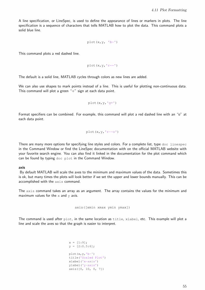
4.11 Plot Formatting

A line specification, or LineSpec, is used to define the appearance of lines or markers in plots. The linespecification is a sequence of characters that tells MATLAB how to plot the data. This command plots asolid blue line.

plot(x,y, 'b-')

This command plots a red dashed line.

plot(x,y,'r--')

The default is a solid line, MATLAB cycles through colors as new lines are added.

We can also use shapes to mark points instead of a line. This is useful for plotting non-continuous data.This command will plot a green “+” sign at each data point.

plot(x,y,'g+')

Format specifiers can be combined. For example, this command will plot a red dashed line with an “o” ateach data point.

plot(x,y,'r--o')

There are many more options for specifying line styles and colors. For a complete list, type doc linespec

in the Command Window or find the LineSpec documentation with on the official MATLAB website withyour favorite search engine. You can also find it linked in the documentation for the plot command whichcan be found by typing doc plot in the Command Window.

axisBy default MATLAB will scale the axes to the minimum and maximum values of the data. Sometimes this

is ok, but many times the plots will look better if we set the upper and lower bounds manually. This can beaccomplished with the axis command.

The axis command takes an array as an argument. The array contains the values for the minimum andmaximum values for the x and y axis.

axis([xmin xmax ymin ymax])

The command is used after plot, in the same location as title, xlabel, etc. This example will plot aline and scale the axes so that the graph is easier to interpret.

x = [1:9];y = [2:0.5:6];

plot(x,y,'b-')title('Scaled Plot')xlabel('x-axis')ylabel('y-axis')axis([0, 10, 0, 7])

55


If we want one of the axis limits to be adaptive then we can use inf instead of a value. This code willbound the lower end of the x-axis to 0 while allowing the upper bound to be set by the data. The y-axis isstrictly controlled as before.

axis([0, inf, 0, 7])

Axis scaling is particularly important if you want to compare two plots. Suppose we plot two lines, eachon a separate plot, without scaling the axes to be the same on both plots. In this case the lines will lookidentical and we will have to read the values on the y-axis in order to distinguish them. However, if wedefine the axes to be the same on both plots then we can easily tell if one of the lines has a steeper slope.As plots become more complex, proper scaling of axes can make them much easier to interpret.

4.12 Naming Index Variables

In the examples above I used idx as the name of the index variable. However, the index variable is just likeany other variable and you can name it whatever you want. This is a perfectly valid sequence of commands,it will return the 4th element from the array.

>>A = [12, 45, 13, 65, 12, 96, 17];>>dragon = 4;>>A(dragon)

Most commonly you will see people use the variable i as the index variable name. In part, this is because iis often used in mathematics as an index subscript. For example, Ai would refer to the “ith” element of A.Also, it’s two fewer key strokes to type i instead of idx. When you’re writing a large program and typingsimilar code over and over again, unnecessarily long variable names get very tedious.

I will note that both i and j are defined in MATLAB just like pi. They both return the imaginary unit,√−1. By redefining them we can override that default value. However, we cannot use that functionality

in a script which is dependent on imaginary numbers. This is almost never a problem, but if you get intoprocess control or certain kinds of robotics then you’ll have to be aware of this issue.

Both i and j are ubiquitous as index variables in coding examples from all languages. In this text I’m goingto use i, j, and k in lots of examples.

4.13 Index Dimension Errors

There are two very common errors which occur while coding for-loops and making plots. These errorsprovide useful feedback to help you get your code working.

Looping

When MATLAB stores an array, it stores exactly as many elements as it has been told to store. Unlike someother programming languages, MATLAB will allow you to add elements to the end of an array. We have

56

4.14 Exercises

done this every time we have made a dependent variable array using a for-loop. The 6th element did notexist before we assigned it.

If an element does not exist, then you cannot access it’s value. So if an array has only 5 elements and ascript tries to access the 7th element then MATLAB will return this error.

Index exceeds matrix dimensions.

You will encounter this while building for-loops. For example, if the independent variable array has only 21elements, but the bounds on the for-loop are set from 1 to 41 (off by a factor of two when you account forfencepost error) then MATLAB would return this error on iteration #22. That will be the first time thatMATLAB attempts to access an element that does not exist.

So the short interpretation is that this error means there is a mistake with the indexing inside the for-loop.Don’t get upset, just go fix it. When the error occurs in a script, the line of code that generated the errorwill be displayed with the error as shown in Chapter 2.

Plotting

When we made our list of points for the manual plot, there were exactly 9 values in each column. It takestwo values to make a point, so if one column had 8 values and the other had 9 values, then we would have avalue which did not have a mate. MATLAB will not make a plot if the two arrays are not the same length.Instead it will return this error.

Error using plot.Vectors must be the same length.

The first step is to check the length of the arrays that you’re trying to plot. Once you know which one isincorrect, you can look at the last assignment of that variable. For example, a common mistake for newcoders is to forget the index variable in the assignment of the independent variable in a loop. They simplyoverwrite a single value with each iteration, and then try to plot the single value vs. the dependent variablearray.

4.14 Exercises

1. Write a for-loop which will count from 0 to 25 by 5’s.

2. Write a for-loop which will count from 5 to 85 by 5’s.

3. In the Command Window, choose 5 numbers and store them in an array. Use the index to print eachindividual value.

4. Create an array with 7 elements. Use the length command to measure the length of the array. Dothese numbers match? Add some more elements and then run the length command again.

5. Write a for-loop which will calculate the average value of all of the elements in an array. Use thisarray to check your algorithm.

x = [2, 4, 9, 5, 1, 6, 3, 2];

57


6. Use the ideal gas law to plot pressure vs. volume of 42 moles of gas at a temperature of 300K. Thevolume should range from 100Liters to 500Liters. Include appropriate axis labels and a title.

7. On the same graph, plot the sine, cosine, and tangent functions on the interval [0, 10π]. Includeappropriate axis labels, a title, and a legend. Use the axis command to scale the axes and make theplot more readable.

8. Plot the cardinal sine function on the interval [−10π, 10π]. Use enough resolution to get a smoothcurve. Include appropriate axis labels and a title. Use the LineSpec to make the line thick and black.

y =sin(x)

x

9. Plot this bouncy function on the interval [0, 10π]. Include appropriate axis labels and a title. Use theLineSpec to make the line thick and red.

y =sin2(x)

x

10. Wavenumbers. The wavenumber, k, denotes the spatial frequency of a periodic signal. In this exer-cise, we’ll plot several wavenumbers of the sine function. The independent variable is multiplied bythe wavenumber to change the frequency as follows:

y = sin(kt)

Follow the steps to plot three different values for the wave number over the specified time domain.

a) Open a new script, make a header comment with preamble commands, and save it as wavenumber.m

b) Create an independent variable, t, with the domain 0 ≤ t ≤ 10π. Use increments of 0.5.

c) Save your script and run it. Make sure the independent variable, omega is stored in theWorkspace. Now, look at the last value. We typed in 10 ∗ pi when we defined it. Are theyequal? Take a look at your increment and see if you can figure out why it rounded down.

d) Create three wavenumber variables, k1,k2, and k3 and assign them values of 0.5,1, and 2.

e) For a single wavenumber, the expression inside the for-loop would look like this:

y(idx) = sin(k*t(idx))

Since we have three wavenumbers, we need three different dependent variables to store the datafor plotting. Let’s call them y1,y2,y3. Using the expression above as a example, construct afor-loop that will evaluate the sine function for each of the three wavenumbers and store theresults in the y array with matching subscript.

y1 = sin(k1t)

y2 = sin(k2t)

y3 = sin(k3t)

58

4.14 Exercises

f) Now let’s plot it with a title, axis labels, and an appropriate legend. We’ll also scale the axesusing the axis command for easier interpretation. In other words, put some white space aboveand below the lines.

Don’t forget the hold on command after the first plot function and that the legend needs to belabeled in the order it was plotted. Run the code here and look at the results. Read the legendand look at the cycling of the lines. See the wavenumber?

g) Play around with the k values a little bit, making them higher and lower, and then examine theresults. What happens if you set two signals to equal but opposite values?

11. Multicomponent Reaction In the guided exercise we used the exponential decay function to predictthe change in a quantity over time. However we only considered a single component. In practicesystems can have multiple components. Consider a chemical reaction.

Reactions have products and reactants and so we need to model both components.

A→ B

Use the following expressions for the concentration of species-A and species-B:

C(A,t) = C(A,0)e−kt

C(B,t) = C(A,0) − C(A,t)

Use an initial concentration, C(A,0), of 10(mg/L), and a rate constant, k, of 0.1hr−1. There is nomeasurable amount of species-B in the system at t = 0. We will plot the function over the domaint = [0, 48]hrs.

59

5 Logical Operations

In Chapter 4 we focused on automating repetitive “plug-and-chug” calculations. This is a common use ofcomputational tools in science and engineering. In this chapter, we’re going to learn to use code to makedecisions. This functionality is widely used to both laboratory and production processes.

Before we dive into the actual decision making, we’re going to learn about basic True/False logic.

5.1 Relational Operators

The familiar inequalities are included in MATLAB as relational operations, using characters which are meantto be readable. The table below summarizes the syntax.


a < b a < b

a > b a > b

a ≤ b a <= b

a ≥ b a >= b

a = b a == b

Note the order of the symbols in the greater than or equal and less than or equal operators. Also notethe double equal sign for testing equality. This is because a single equals sign is used to assign values tovariables. Recall that we refer to the single equals sign as the assignment operator.

Generally algebraic inequalities are interpreted to be true. In contrast, programmatic relational operationsevaluate a relationship and then return True or False.

Type the following expression into the Command Window and press Enter .

>>5 < 7

Now look at the output. You’ll see the familiar default variable name, ans, but the value assigned is 1and the word logical is printed above. Up to this point, all of the other numerical variables we’ve usedhave been doubles. A logical is a variable which can only be true or false. It is standard practice amongall programming languages to use 1 for true and 0 for false. The output from a relational operator is alogical which indicates whether the expression is true or false. Let’s test out a false expression to see thedifference.

>>5 > 7

Now the logical has a value of 0 because the expression is false. We can also name logicals, just like we canwith doubles, using the assignment operator.

61


>>a = 5 < 7

Try these shorts exercises to gain familiarity with the relational operators in MATLAB.

1. Make up some numbers and experiment with the > and < relational operators in the CommandWindow. Choose numbers so that you produce both true and false output for both operators.

2. Now test the ≥ and ≤ operators. Test both possibilities for a true output, and generate a false outputas well.

3. Finally, test the equality operator using ==. Generate both true and false output. Also, what happensif you use a single equals sign?

5.2 if-statements.

Often we will write code which we only want to execute under certain conditions. An if-statement is acontrol structure which uses a logical to determine whether or not to run a block of code. Basically, if thelogical is true, then the code runs, and if the logical is false, then the code does not run.

The structure of an if-statement looks like this.

if 1% <some code>% <some more code>

end

In this example, the code in the middle will run because the logical is true. Note that the if-statement isclosed with the end command, just like the for-loop. To prevent the code from running, the logical is setto false.

if 0% <some code>% <some more code>

end

While this basic functionality is useful sometimes, more often we want to use this control structure to makea decision which will depend on an unpredictable input. Luckily, the relational operators output a logicalwhich can be interpreted by the if-statement. We can replace the strict true/false coding above with aconditional statement that will evaluate differently depending on the input.

if a < b% code% more code

end

62

5.3 Looping with if-statements.

Now, the code inside the if-statement will execute if the expression evaluates as true, and will not executeif the expression evaluates as false. We can write a very simple script to study this concept.

Create a new m-file, save it with an appropriate name, and make a header comment. Then enter thefollowing commands:

% This script demonstrates the basic% functionality of an if-statementclear all; close all; clc;

a = 3;b = 7;

if a < ba + b

end

Run the script. What was the output? Now change the value of a and b so that the relational operation willevaluate to false. In other words, make a greater than b. Run the script again. What was the output? Goahead and try some experiments with the other relational operators. Once you’re comfortable work throughthe following exercises to practice building simple if-statements.

To practice, write a short script which evaluates a variable, T, and prints “Too Hot!” to the commandwindow if the value is greater than 300. Use the disp function to print the character string like this:

disp('Too Hot!')

Once you’ve completed the script, try several values of T to produce both true and false results.


We can use if-statements inside for-loops to automate decision making. In this section we’ll build a simplefor-loop to find the largest value in an array. Let’s use the template from Chapter 3 to develop a solutionfor a specific case. Once the algorithm is verified we can implement the solution in MATLAB and run somemore tests.

GivenAn array of random numbers.

A = [1, 4, 76, 42, 7]

FindFind the maximum value in the array using a reproducible algorithm.

AssumptionsThe array may contain all real numbers.

SolutionIn this simple case, we can just look at the array and determine the largest value. The brain is very well

63


adapted to comparisons and so we don’t even consciously apply a particular method, we just look at theshort list and “know” that 76 is the largest value.

Unfortunately this method does not scale. For instance, if I said that I was going to show you 100 flashcards exactly one time each and then ask for the largest number, you might have to come up with a betterstrategy than “just look at it.” If 100 still seems manageable, consider 1,000, or 10,000. At some point youwill no longer be able to remember the highest value.

In this case, there is a simple solution. You can just grab a sheet of paper (or open a text editor), and makenotes about the highest value that you have encountered so far. The basic method takes two steps.

1. Determine if the number on the current flash card is largerthan the current largest value in your notes.

2. If so, write down the current flash card value in your notes.If not, look at the next flash card.

Each time you encounter a larger number you will make a note. All cards with smaller values will bediscarded.There is a special case. When you look at the first flash card, you won’t have anything written inyour notes, so you can’t compare it to anything. In this case, the value on the first flash card becomes thehighest value by default.

This method scales simply. Obviously it will take more time to do more flash cards, but you wouldn’t haveto make any changes to the underlying process. It also doesn’t depend on any high level interpretation. Thisis exactly the sort of method we can easily implement in a MATLAB program.

So far we’ve learned about storing arrays and single values, retrieving elements with indexing, and loopingthrough repetitive problems. Now we can add a basic if-statement to the mix and solve this problem.

Let’s write down the steps of the “Flash Card” algorithm using some basic MATLAB terminology.

1. Define the array. This is the virtual deck of flash cards.Each element will be the equivalent of one card.

2. Initialize a variable to keep track of the largest value. Itshould be named something obvious like max value. Assignit the value of the first element. This is the equivalent ofnoting the value of the first flash card as a reference.

3. Get the value of the next element. This is the flipping ofthe next card.

4. Compare the element value to max value. Is it larger?Then assign the element value to max value.

5. Repeat steps 3-4 until the end of the array.

This is a flow chart of the algorithm above.

64


Figure 5.1: Flow chart for the algorithm to find the largest element in an array.

Each time that the relational operator encounters an element that is larger than the max value variable, thevalue of max value is overwritten with the value of that larger element.

Let’s go through the algorithm step by step using the example array above.

1. We have the array defined already, so we can move on to the third step.

2. We set max value = A1

3. The second element is 4.

4. Is 4 > 1? Yes, so we set max value=4.

5. The third element is 76.

6. Is 76 > 4? Yes, so we set max value=76.

7. The fourth element is 42.

8. Is 42 > 76? No, so the value of max value stays at 76.

9. The last element is also less than 76, so the algorithm is finished and max value is set at 76.

MATLAB Implementation

1. Create a new script, save it with an appropriate name, and make a header comment. Include apreamble as well.

65


% find max value.m

% This script finds the maximum value% of the elements in an array.

% preambleclear all; clc;

2. Define the array.

% define arrayA = [1, 4, 76, 42, 12];

3. Initialize the max value variable with the first element.

% initialize max valuemax value = A(1);

4. Now for the for-loop. We will iterate through each element of x and check it against max value

using an if-statement. Note that we start with the second element since the first has already beenstored. It won’t change the answer if we start at the first index, but it’s a wasted step since we alreadyhave the value stored.

% loop through elementsfor i = 2:length(A)

% if element is greater than max valueif A(i) > max value

% assign element value to max valuemax value = A(i);

% end if-statementend

% end for-loopend

The if-statement controls the assignment for max value. It will only occur if the current elementvalue is less than the current value of max value. Each time through the for-loop is the equivalentof turning a flash card, and each encounter with the if-statement is the equivalent of comparing theflash card to your list and recording a higher value (or not).

5. Display the raw data and the largest value in the Command Window.

% report resultsdisp('Array values:')disp(A)disp('Maximum value:')disp(max value)

66

5.4 if-else-statements.

At this point the script should scale very well. Try a few different arrays. What happens if you define anarray of negative numbers?

5.4 if-else-statements.

Often we’ll want to combine multiple decisions into a single program. MATLAB offers many options toaccomplish this. In this section we’ll learn about if-else-statements. The structure of an if-else-statements is as follows:

if a < ba + b

elsea - b

end

Initially, the relational operation will be evaluated and the if-statement will interpret the logical. If thelogical is true, then the first block of code (a + b) will execute and the second block of code will be skipped.If the logical evaluates to false then the first block of code will be skipped and the second block of codewhich occurs after the else-statement (a - b) will execute. The code which follows the else-statementwill always execute if the relational operation evaluates as false. Let’s use an if-else-statement to expandon the temperature warning we built in Exercise 2.

Let’s see it in action with this script which will evaluate a variable, T, and print “Too Hot!” to the CommandWindow if the value is greater than or equal to 300, and “Just Right!” under other conditions. Try severalvalues of T to test out your code.

% This script checks a temperature% and returns a message based on% the value.

% preambleclear all; clc;

% define TT = 325;

% check the condition% and print messageif T > 300

disp('Too Hot!')else

disp('Just right!')end

5.5 if-elseif-else-statements

Sometimes we want to combine more than one conditional statement. To build on the example above,it might be useful to identify temperatures that are either too hot or too cold. In this case, we use an

67


if-elseif-else-statement. The syntax is very similar to an if-else-statement. Let’s look at a simpleexample.

% define TT = 325;

% check the condition% and print messageif T > 300

disp('Too Hot!')elseif T < 275

disp('Too Cold!')else

disp('Just Right!')end

Now there are three options which depend on the value of T. Just like if-else-statements, only 1 of theexpressions will execute. If the first statement is true, then MATLAB will only run the commands under thatif-statement. The other two will be skipped entirely. If the if-statement is false, but the elseif-statementis true, than only the code under the elseif will execute.

We can stack up as many elseif-statements as we need, but since only one will execute we must paycareful attention to the order. Consider this short problem.

A = 10;B = 5;

if A < 25% some code

elseif A < 15% some code

elseif B > 2% some code

else% some code

end

All of the relational operations will evaluate as true, but only the first section will execute. If an algorithmrequires a complex structure, then care must be taken to make sure that the statements are in the correctorder. That said, if you ever find yourself trying to use a double digit number of elseif statements, it’smost likely time to reconsider your approach to the problem.

5.6 Testing Data

Testing an algorithm requires data. It’s not always convenient to use real data for testing, and in somecases it can make the troubleshooting process more difficult. In many cases it is preferable to generate someartificial data the resembles the real data that you will eventually process.

MATLAB includes many tools for generating data. One of those tools is the rand function, which generatesa random number between 0 and 1. Try it out in the Command Window.

68

5.7 Boolean Operations

>>rand

Now run it again. The number will be different. Since there is an algorithm generating the number, it’snot truly random. If you knew the algorithm and could measure all the inputs, then theoretically you couldpredict the number. Since we don’t know any of that stuff, for our purposes the numbers are sufficientlyrandom.

The function returns a number between 0 and 1. If we want a number between 0 and 10, we can simplymultiply the output of the function by 10.

>>10*rand

If we want to return a random number between an upper and lower bound, we can use this formula.

% define boundslow = 5;high = 10;

% get random numberx = low + (high-low)*rand

Can you see how it works? The sequence (high-low) calculates the difference between the upper andlower bound. Multiplying it by the rand function scales it by a factor between 0 and 1. The scaled quantityis then added to the lower bound. If rand returns a number close to 1, then x is close to the upper bound.If rand returns a number closer to 0, then x is closer to the lower bound.

We can also create an array of random numbers by specifying the number of rows and number of columns.Since we are only using row arrays at this point, we can make an array of random numbers with 1 row and10 columns. This will result in a row array with 10 elements.

rand(1,10)


In Section 5.1, we learned that relational operations produce a logical variable type. We can perform avariety of operations on logicals, and those operations are called Boolean operations. Boolean operationsform the entire foundation of electrical computing, from the most basic 4-function calculator to the mostadvanced super-computer. In this section we’ll learn to use two Boolean operations to combine relationaloperations.

Just like the other familiar mathematical operators, Boolean operators act on elements to produce otherelements in the same space. Since the Boolean space is limited to true and false, boolean operations act onmultiple logicals, and then produce another logical. In this studio we will only use two Boolean operations,AND and OR.

69


ANDThe AND operator returns true if both logicals are true.

true AND true = true

true AND false = false

false AND false = false

The MATLAB syntax for the AND operator is the double ampersand (&&). Try the following example inthe Command Window for clarity.

a = 5

a < 10 && a > 2

MATLAB will return a logical which is set to true (1). Now change the value of a such that one of therelational operations evaluate as false and then rerun the second line of code.

ORThe OR operator returns true if either of the logical variables are true.

true OR true = true

true OR false = true

false OR true = true

false OR false = false

The MATLAB syntax for the OR operator is the double vertical bar ( || ). Try the following example in theCommand Window for clarity.

a = 5

a < 10 || a > 12

MATLAB will return a logical which is set to true, despite the fact that the second relational expressionevaluates to false. Now change the value of a such that both of the relational operations evaluate as falseand then rerun the second line of code.

Why is this important? In many practical cases we have multiple conditions to meet. What if we want toknow if a number is greater than 5 and less than 10. Algebraically we would write an expression like this.

5 < x < 10

However, if we type a similar expression into the Command Window MATLAB will not interpret it correctly.This is because MATLAB reads from left to right once order of operations have been considered. Todemonstrate, let’s work through a quick exercise.

First define a variable x which meets the criteria.

>> x=7;

Next we’ll try to replicate the expression above.

70


>> 5 < x < 7

The result should be a logical set to 1 (true). This is technically a correct result and it could be temptingto assume that the expression works, but it turns out that it returns a correct answer for the wrong reasonand will fail in obvious cases. Try this nonsensical expression.

>> 5 < x < 2

It also returns true! How can that be? There is no number that can be both greater than 5 and less than2. But MATLAB is reading left to right. At the first operator, it evaluates whether 5 is less than 7. That istrue, so MATLAB simply stores the result (1) and moves on to the next operation. Now, because MATLABis dynamically typed and allows variable to switch types in certain cases, it decides to use 1 as a doublerather than a logical. In other words, it simply asks if 1 is less than 2, and it is, so the final result is true.

To prove this point, change the last number to 0.

>> 5 < x < 0

Now it’s false, because in the last step is asks if 1 is less than 0.

The point is, if you are ever constructing an if-statement to implement a complex inequality you must useboolean operations to get a correct evaluation.

In the last section we learned to make an array of random numbers between 0 and 1. This example will loopthrough the numbers and print only the ones that meet this inequality.

0.25 < x < 0.75

Since our variable needs to be inside the range, we use the AND operator. The number must be greaterthan 0.25 and less than 0.75.

x = rand(1,10)

for i = 1:length(x)

if x(i) > 0.25 && x(i) < 0.75disp(x(i))

endend

If the inequality was reversed, we would be filtering outside of the bounds.

0.25 > x > 0.75

In this case, we would use the OR operator, because a number cannot be less than 0.25 and greater than0.75.

71


x = rand(1,10)

for i = 1:length(x)

if x(i) < 0.25 | | x(i) > 0.75disp(x(i))

endend

5.8 Errors & Troubleshooting

There is one error that is definitely the most common when dealing with if-statements. It occurs when asingle equals sign is used to measure equality. Recall that the single equals sign is the assignment operatorand it has a specific purpose. The double equals ( ==) is used to measure equality.

An incorrect if-statement like this:

if a = b% some code

end

Will return an error like this:

The expression to the left of the equals sign is nota valid target for an assignment.

There are other issues that arise from relational operations which do not generate errors but still mess upthe algorithm. When using relational operations inside loops to check values in an array, it’s a commonmistake to forget to index the array in the conditional statement. See this example below.

A = [1:10];B = 3;

if A > Bdisp('True')

end

In this case MATLAB will not generate an error. This is because the relational operators can operate onan entire array. We’ll discuss this in detail in Chapter 10. It’s just important to know that if the operationis false for any element, then it will be interpreted as false by the if-statement. Even though most of A isgreater than B, this code will not print to the Command Window at all. Instead, the correct approach is toloop through the array element by element, and compare them one at a time using the index.

72

5.9 Exercises

5.9 Exercises

1. In the Command Window, validate all of the relational operators by choosing numbers to generateboth True and False results.

2. Write a short script which will evaluate a variable x and print “Negative!” to the Command Windowif the value is less than zero.

3. Write a short script which will evaluate a variable x and print “Positive!” to the Command Windowif the value is greater than zero.

4. Write a short script which will evaluate a variable x and print “Negative!” to the Command Windowif the value is less than zero and “Not Negative!” for other values.

5. Write a short script which will evaluate a variable x and print “Negative!” to the Command Windowif the value is less than zero and “Not Negative!” for other values.

6. Write a script which will loop through the elements of an array and print only the elements which aregreater than 5 to the Command Window. Use this command to generate the array for evaluation.

data = 10*rand(1,10);

7. Write a script which will plot sine and cosine functions over the domain [0, 10π]. Use a red line forthe sine function and a green line for the cosine function.

Difficulty: Round all negative numbers to zero before plotting

8. Using boolean operations, write a command that will confirm that a variable y is greater than 25 andless than 35. Validate the command in the Command Window using several values for y. Be sure totest values below 25, above 35, and also in between.

9. Using boolean operations, write a command that will confirm that a variable y is less than 65 orgreater than 80. Validate the command in the Command Window using several values for y. Be sureto test values below 65, above 80, and also in between.

10. Write a short script which will evaluate a variable, T, and print “Too Hot!” to the Command Windowif the value is greater than 99.6, “Too Cold!” to the Command Window if the value is less than 97.6,and “Just Right!” to the Command Window if the value is in between. Validate the script with severalvalues of T.

11. Write a short script which will loop through the elements of an array and print “Small” to the CommandWindow for elements less than 1, “Medium” for elements that are between 1 and 2, and “Large” forany element above 2. Use this command for data.

data = 3*rand(1,10)

How do the results change if we change the input data?

data = 6*rand(1,10)

73

6 Nested Loops

In Chapter 4, we learned to use for-loops to automate repetitive calculations. In Chapter 6 we’re going toexpand on that concept by nesting loops. Nesting simply means that we will put a loop inside of a loop.But first, we will learn about two dimensional arrays.

6.1 Indexing in Two Dimensions.

Arrays can have more than one dimension. We access individual elements by using one index for eachdimension. For example, to access elements in a two dimensional array, we need two indices. One indexidentifies the row number, and the other identifies the column number. Consider the 3× 3 array below.

A =

a1,1 a1,2 a1,3a2,1 a2,2 a2,3a3,1 a3,2 a3,3

The first subscript identifies the row, and the second identifies the column. An m× n array would have mrows, and n columns, as shown below.

A =

a1,1 a1,2 · · · a1,na2,1 a2,2 · · · a2,n

......

. . ....

am,1 am,2 · · · am,n

Just as before, the MATLAB syntax is meant to mimic the underlying mathematics. To access an individualelement, we use similar syntax to the 1-D case. The difference is that now we have to pay attention to therow number and the column number. This command will return the element in the second row and thethird column from an array called A:

>>A(2,3)

We can also remove whole rows or columns from the array using the colon operator. The following commandwill return the whole second row:

>>A(2,:)

Similarly, this command will return the whole third column:

>>A(:,3)

75

6 Nested Loops

When we use the colon operator to generate an array, it will count from the lower number to the highernumber by an increment of 1. By indexing with the colon operator, the upper and lower bounds are assumedto be the first and last index. We can specify a limited range by explicitly entering the upper and lowerbounds. This command will return the 2nd, 3rd, and 4th element from the 2nd column.

>>A(2:4,2)

To enter a two dimensional array into MATLAB, the semicolon operator must be used to separate the rows.The following syntax will create a 3× 3 array named A:

A = [1, 2, 3;

4, 5, 6;

7, 8, 9]

We have previously only used the semicolon operator to suppress the output of a command to the CommandWindow. This is an example of what I’m going to call “context specific syntax.” Basically, MATLAB can tellif the semi-colon is at the end of a command, or part of an array. It chooses a different operation for eachsituation. If the semi-colon is at the end of a command, then it suppresses the output. If the semi-colonis in an array, then it makes a new row. It’s a little confusing at first, but with practice it becomes secondnature.

We don’t actually have to type the rows on separate lines. The semicolon will make the rows automatically,so we can type short arrays one line. Try this in the Command Window.

>> A = [1 2; 3 4]

Try this exercise to solidify your understanding.

1. The magic command returns a square 2-D array. The numbers are the same every time so you canuse it for learning. Try this in the Command Window.

>>A = magic(5)

2. Use the indices to return individual values. Practice until you can visually pick a value from the arrayand consistently return it.

3. Use a combination of an index and the colon operator to return entire rows and columns.

4. Now try taking a slice out of one row or column by defining the upper and lower bounds around thecolon operator.

5. Practice until you are confident that you understand two dimensional indexing!

6.2 Nested for-loops

A nested loop is a loop inside of another loop. We most often use nested loops to iterate over the elementsof arrays with more than one dimension or to perform combinatorial simulations. Before we look at some

76

6.2 Nested for-loops

examples, let’s examine exactly how the indices change within a nested loop. Try this simple script in thecommand window. We’ll iterate through two index variables and save them in an array at each iteration,then we can print the array to the Command Window and easily see how the index variables are changingrelative to each other.

for i = 1:3for j = 1:3

% save the index variables% in an array for displayx = [i,j]disp(x)

endend

The inside loop will execute completely during each iteration of the outer loop. In other words, each timeMATLAB encounters a loop, it finishes the loop completely before moving on. The result is that the firstiteration of i experiences all three values of j. When the outer loop begins, i is set to 1. Then MATLABencounters the inner loop and j is set to 1. Once the inner iteration is complete, j is set to 2 but i remainsat 1 because we are still on the first iteration of the outer loop. This can be seen in the output of the codeabove. The first element, which is the value of i is 1 for the first three lines as the second element, whichis the value of j, counts from 1 to 3. Then the value of the first element goes up to 2, indicating that thesecond iteration of the outer loop has begun.

I recommend that you implement the code above and change the intervals to gain intuition about thebehavior of nested loops

6.2.1 Counting With Nested Loops

Suppose we have 3 apples and 4 oranges. Assuming the fruit stays whole, how many combinations of fruitcan we make?

This is an easy problem to solve without the computer, but it clearly demonstrates the behavior of thenested loop. If we think through the process, we can have 1 apple and 1 orange, 1 apple and 2 oranges, etc.We can use one loop to represent the count of the apples, and a loop inside to represent the count of theoranges. Each time that the inside loop iterates, it will represent one combination. A variable which countsthe total number of iterations will tell us the number of combinations.

% initialize countercount = 0;

% loop through fruits% and update counterfor apples = 1:3

for oranges = 1:4count = count + 1;

endend

disp(count)

77

6 Nested Loops

6.2.2 Nested Wavenumbers

In the next section, we’ll focus on the methodical construction of nested loops. It will help to have a highlevel understanding of what is happening before we try to build one from scratch. Look at this example andthen read the explanation. It is an extension of the guided wavenumber exercise in Chapter 4.

% nested wavenumbers.m% This script plots the wavenumber tutorial% using a nested loop to change the value of k.clear all; close all; format compact; clc;

% define wavenumbersk = [0.5, 1, 2];

% define independent variable arraytheta = [0:0.01:4*pi];

% loop through wavenumbersfor k idx = 1:length(k)

% loop through thetafor t idx = 1:length(theta)

% calculate the functiony(t idx) = sin(k(k idx)*theta(t idx));

end % end theta loop

% plot the current lineplot(theta,y)hold on;

end % end k loop

% format the plottitle('Wavenumbers')xlabel('x-axis')ylabel('y-axis')legend('0.5', '1', '2')

First, we have the wavenumbers defined as elements in an array. Next we see the familiar independentvariable, theta. In the middle of the script we see two for-loops, one inside the other. The inner looplooks very similar to the loop from the wavenumber script in Chapter 4. However, we can see that there isonly one expression and both k and theta have index variables. If we look at the for-loops, we can seethat the index variables have names which correspond with the arrays that they are indexing.

When the script is executed, the first value from the wavenumber array will be used to evaluate the sinefunction over the domain [0 ≤ θ ≤ 4π]. Once the inner loop exits, then the result will be plotted. Thehold on command will be called so that future plots do not overwrite. Then the outer loop will start overagain, and the second value of the wavenumber array will be selected and another line calculated and addedto the plot. After the final iteration of the outer loop, the loop will exit and any code below that loop inthe script will execute.

Note that we mark the end of the loops with identifying comments. This allows us to easily understand thestructure later.

78

6.3 Ideal Gas Law Isotherms

Go ahead and recreate the script. Experiment with the domain and the wavenumbers to get some intuitionabout the operation. In the next section we will build our own nested loop from the ground up.

6.3 Ideal Gas Law Isotherms

In this section we will work through the process of building a nested loop to plot several lines on a singleplot. It’s a more complex procedure that building single for-loops, so for best results we will break theprocess into steps.

ProblemIsotherm means constant (iso) temperature (therm). It is often useful compare the behavior of a system atseveral different constant temperatures in order to understand the influence of several parameters. Considerthe ideal gas law.

PV = nRT

If we assume that the amount of gas (n) is fixed, then there are three variables, P ,V , and T . A standard 2Dplot has only two axes. If we want to represent a system with three dimensions on a two dimensional plot,we have to use multiple lines to represent one of the dimensions. We saw this in the previous wavenumberexample. The wavenumber was represented using separate lines rather than an axis on the plot.

Let’s write a script to plot P vs. V for several values of T.

For the volume we’ll use a domain of:

10 liters ≤ V ≤ 100 liters

For temperature, we’ll go from 200K to 700K in increments of 100K.

The inner loop will be a standard P − V calculation like we’ve seen in the exercises. However, this timewe’ll use an outer loop to pass in different values for the temperature.

It’s difficult to construct a nested loop without first testing the inner loop. For this reason it’s best to writethe script with the inner loop only, and then add the outer loop after the inner loop has been confirmed tobe correct. We will start by plotting a single P − V curve. Since we’ve done this in a previous exercise itshouldn’t take too much effort.

79

6 Nested Loops

% ideal isotherms.m% This script plots the P-V curve% using the ideal gas law.clear all; close all; format compact; clc;

% define the temperatureT = 300; % (K)

% amount of gasn = 1 % (mol)

% universal gas constantR = 8.314 % (J/(mol*k))

% define volume arrayV = [0.01:0.001:0.1]

% loop through volumefor i = 1:length(V)

% calculate pressureP(i) = (n*R*T)/V(i)

end

% plot resultsplot(V,P)xlabel('Volume')ylabel('Pressure')

This code plots a single P − V curve at a temperature of 300K. Once it is confirmed to run without errorswe can think about implementing the outer loop.

In the previous example, the calculation for a single sine wave was wrapped in an outer loop update thatwavenumber and plot separate lines. In this case we’re going to wrap our P − V for-loop in an outer loopwhich will update the temperature and plot several isotherms on one graph.

There are three steps to this process.

1. Create an array of temperature values to replace the single value.

2. Write the outer loop code. The for command will be before our current loop and include the indexvariable for the T array. The end command will fall after the plot command. This is because wewant to plot each curve after we calculate it. Since the P array is being overwritten each time theouter loop executes, we need to plot the current values before we start the inner loop over again.

3. Update the reference to the T variable in the pressure calculation to reflect that we are indexing anarray.

The first step is easy since we were given a range in the problem statement. After completing the array, weneed to move on to step 2. This involves selecting an index variable. In this case, since i was already used,I am choosing something completely different, m. In some cases, it might even be useful to name the indexvariable after the array which it is indexing. In this case T idx and P idx would be fine name.

After making the changes to our script, it should look something like this.

80

6.4 Plotting in 3D.

% ideal isotherms.m% This script plots the isotherms of the ideal gas lawclear all; close all; format compact; clc;

% define the temperature arrayT = [200:100:700] % kelvin

% amount of gasn = 1 % mol

% universal gas constantR = 8.314

% define volume arrayV = [0.01:0.001:0.1]

% loop through temperaturefor m = 1:length(T)

% loop through volumefor i = 1:length(V)

% calculate pressureP(i) = (n*R*T(m))/V(i)

end

% plot inside the outer loop% to capture each lineplot(V,P)hold on

end

% format plotxlabel('Volume')ylabel('Pressure')legend('100','200','300','400','500','600','700')

6.4 Plotting in 3D.

In this section we’ll utilize a nested for-loop to plot an interesting 3 dimensional function.

z =sin(√

x2 + y2)

√x2 + y2

Since we have to independent variables, x and y, we need to use a nested loop to iterate through each ofthem. The resulting z array will be 2-dimensional. For now we’ll use the interval [−6π, 6π] for both x andy.

81

6 Nested Loops

% bounce 3D.m% This script utilizes a nested for-loop% to plot an interesting 3D surface.clear all; close all; format compact; clc;

% make arrays using variables for easy scalingscale = 6;incr = 0.5;x = [-scale*pi:incr:scale*pi];y = [-scale*pi:incr:scale*pi];

% loop through the columnsfor y idx = 1:length(y)

% loop through the rowsfor x idx = 1:length(x)

% calculate the functionz(x idx,y idx) = sin(sqrt(x(x idx)ˆ2 + y(y idx)ˆ2))/sqrt(x(x idx)ˆ2 + y(y idx)ˆ2);

endend

% plot surface and save handles = surf(z);

% use handle to set edge colors.EdgeColor = 'None';

The x and y arrays are defined using variables. This allows for easy scaling. If we only want to view thefunction over the interval of [−3π, 3π], then we can simply change the scale variable to 3. Similarly, ifwe want more resolution in the independent variables, we can make the incr (short for increment) variablesmaller.

The nesting loop will store the values in a 2D array called z. Afterward we can use the surf command toplot the 3D surface.

In this case, we are also assigning a variable name to the plot. This is called a plot handle and it allows usto make changes to the plot after it has been made. Some of the changes that we can make to plots areonly available through a handle. In this case we want to turn off the edge color and to do that we need touse a handle.

The reason we are turning off the edge color is that at high resolution the black lines on the surface plotwill cover up the color and make the plot unusable. To demonstrate this, remove the last line of code fromthe script and run it. Now change the increment to 0.01 and run it again. See the difference? That’s whywe turn off the edge color.

6.5 Nested Sums.

This is another guided exercise. I will provide instructions and certain segments of code, but you will haveto piece the solution together yourself.

This is a simple task to understand. We’re just going to sum to columns in an array. Think of it like aspreadsheet where we calculate totals at the bottom of each column. We’re going to use a couple of new

82

6.5 Nested Sums.

commands, but they are very similar to other commands we have use. Follow the steps to create your owncolumn summing script.

1. Open a new script, save it with an appropriate name, make a header commend and preamble.

2. Use the following command to make a 2D array of random data. Remember the rand function acceptsinput for the number of rows and the number of columns, so our output array will have 8 rows and 5columns.

data = rand(8,5)

3. Run the script and look at the data and the Command Window. You can see that data is an 8x5double. To get a better view, type data at the prompt in the Command Window.

4. Type doc size into the Command Window and read the documentation. You will see that it operatesjust like the length function except that it acts on 2D arrays. It will return the number of rows andthe number of columns. Try this in the Command Window.

>> size(data)

You will see that it returns two values in an array. The first value is the number of rows, the secondvalue is the number of columns. We can even store these results with descriptive variable names.

[n rows,n cols] = size(data)

The size command allows us to automate indexing in 2D arrays the same way that the length

command allows us to automate indexing in 1D arrays.

5. We will also need a variable to store the sums. Remember how we defined a counter variable whensumming a 1D array? Well now we have to do that for all 5 columns, so we’re going to need an arrayswith 5 elements that all start at zero. Fortunately we can use the zeros command to make an arraywith a value of zero in every element. The zeros command works a lot like the rand function in thatwe can input the number of rows and columns. In this case, we’ll make an array called total with 1row and the same number of columns as data.

total = zeros(1,n cols);

6. Now choose one column and write a single for-loop to sum the elements in that column and storethem in the corresponding element in total. This will eventually be the inner loop. If you havetrouble, consult the section on 2D indexing. To get you started I will give this short loop which willdisplay the value of each element in column 2 of data. You can modify it to sum the values usingthe total array.

for i = 1:n rowsdisp(data(i,2))

end

Be sure to look at the values in total after you run your script. Is the sum saved in the secondelement? Is it correct? If so, then move along to the next item.

7. Now that the inner loop is working, wrap it in an outer loop that iterates over the columns. Youalready have a variable for the number of columns, so adding this loop is fairly straightforward.

83

6 Nested Loops

8. Report the results to the Command Window.

6.6 Exercises

1. Suppose you have 3 quarters, 2 nickles, and 4 pennies. Use a nested for-loop to count the maximumnumber of combinations of the coins.

2. Use a nested for-loop and the surf command to plot this 3-dimensional function. Find an interestinginterval for the independent variables.

z =sin(x)cos(x)

2

3. Use a nested for-loop and the surf command to plot this 3-dimensional function. Find an interestinginterval for the independent variables.

z =√x2 + y2

84

7 Formatted Output

Performing an accurate calculation is only part of building a good simulation or data processing script.Reporting output variables in a useful format is equally important. If it’s difficult to interpret results, or totransfer data to other software, then the utility of the script is greatly reduced.

In this chapter were going to focus on text formatting. We’ll practice printing formatted reports to thecommand window. We’ll also learn to write data to text files.

7.1 Strings

Computers have to store text with variables. The variable type that is used to store text is called a string,which is short for character string. In the workspace, MATLAB uses the abbreviation char.

We create a string by using apostrophes around some text. Then it can be assigned to a variable using theassignment operator.

school = 'Oregon State University'

One way to think about a string is as an array of characters. You can return individual elements from astring using an index.

school(4)

We can use variables to pass strings into any function which accepts a string as an argument. For example,we might pass the title of a plot into the title function like this

% define the titleplot title = 'Acceleration vs. Time'

% make the plot and% add the titleplot(a,t)title(plot title)

7.1.1 Concatenation

Concatenation is an operation which joins arrays. As you progress in your engineering career and use morecomplex mathematics you may find yourself concatenating arrays of numbers, but it’s very common to useit when dealing with text.

85

7 Formatted Output

We’ve actually done some concatenation already without mentioning it. Each time we used a comma ( ,)to separate the values we typed into an array, we were concatenating horizontally. Later on in Chapter 6 weused the semicolon ( ;) to make the rows of the 2-D array. In that example, the semicolon was concatenatingvertically.

Vertical concatenation can be tricky with text, so we’re going to focus on horizontal concatenation. Thiscode joins three short strings into one long string. The output is shown for clarity.

>> A = ['Oregon','State','University']

A =

OregonStateUniversity

Spaces are characters in a string. If we want the output to be readable we need to include some spaces in theconcatenation. We just use some apostrophes around the white space and some commas to concatenate.

>> A = ['Oregon',' ','State',' ','University']

A =

Oregon State University

In the next section, we’ll learn how to inject numbers into strings.

7.1.2 num2str

We’re most often interested in numerical results when using MATLAB. Text is used to improve the inter-pretability of those results. If we output temperature and pressure from a script, it’s nice to have themlabeled with something readable. This is especially true for scripts which are used by people who did notwrite them. If you build a tool for an equipment technician, that person needs to be able to instantlyunderstand the output without having to dig through the code.

When we formatted output in earlier scripts, we simple used the disp command to print the label on theline above the numerical value. Using the function num2str, we can convert a number to a string and thenconcatenate the strings into a single variable for output.

% define numerical variableT = 300;

% convert to stringT = num2str(T);

% concatenate outputout = ['Temperature: ',T];

% return resultsdisp(out)

86

7.2 fprintf

7.1.3 strcmp

Sometimes it’s useful to compare strings and see if they are the same. This is most useful when dealingwith large data sets. If the labels are text, then you need to be able to search by text in order to findthe appropriate entries. Since strings are arrays of characters, the equality operator (==) will compare eachindividual character and return an array of true false values. We could search through this array and concludethat the strings are the same if there are no false values, but this is a clunky and tedious solution. MATLABhas a simple built-in function specifically for comparing strings. The strcmp function accepts two stringsas input and then returns a logical indicating whether or not they are the same. Try this in the commandwindow.

>> a = 'MATLAB'>> b = 'MATLAB'>> strcmp(a,b)

The output is the familiar logical set to 1. Now we can change one of the strings and try it again.

>> a = 'MATLAB'>> b = 'Not MATLAB'>> strcmp(a,b)

The strcmp function is case sensitive and also sensitive to white space. Try these commands to demonstrate.Note the leading space in the assignment of c.

>> a = 'MATLAB'>> b = 'Matlab'>> c = ' MATLAB'>> strcmp(a,b)>> strcmp(a,c)

7.2 fprintf

MATLAB contains some more advanced tools for creating strings. One of the most powerful is fprintf.The name is short for formatted print function, or something along those lines. This function allows formuch more control over the formatting. It also allows us to write to text files instead of simply printing tothe Command Window.

7.2.1 Basic Formatting

In the last section we created individual strings and then joined them together. With fprintf we will createa template and then pass variables into the template using format specification. Consider the temperatureoutput we discussed. The output looked fine because the number we assigned to the variable T was a wholenumber. If the number is not whole, then MATLAB’s auto formatting will kick in. Try this example to seewhat I mean.

87

7 Formatted Output

T = 375/5.73;T = num2str(T);out = ['Temperature: ',T];disp(out)

The output has 4 decimal places by default, but that’s too many significant figures. It would be moreappropriate to print the result with only a single decimal place, which we can do using fprintf.

T = 375/5.73;

fprintf('Temperature: %.1f', T)

This is the most advanced line of code that we have encountered so far. Let’s break it down and examine allthe pieces. The fprintf function accepts two input arguments. One is the string with format specification,the other is the input variable. The function will print the variable in place of the format specification in thestring.

The code %.1f is the format specification. There are 3 separate commands in this piece of code. The % tellsMATLAB where to print the number as a string. This is another example of context specific syntax. Insidea format specification it represent the location of the first digit or character of the string to be inserted.Outside of a format specification it is the start of a comment. The f tells MATLAB to print the number asa floating point decimal. This is what we typically think of as decimal notation. The .1 tells MATLAB toonly print one number after the decimal place.

If we leave out the decimal option in the middle, MATLAB will print the default floating point format.

T = 375/5.73;

fprintf('Temperature: %f', T)

If we wanted 2 decimal places instead of 1, then we would use the option .2 in the middle.

T = 375/5.73;

fprintf('Temperature: %.2f', T)

We can also control the number of digits before the decimal. If we wanted to pad all the output with leadingzeros (which is sometimes useful for formatting data) then we could type something like this.

T = 375/5.73;

fprintf('Temperature: %5.2f', T)

88

7.2 fprintf

There are other format specifiers besides %f. We can use %d to print a number in engineering notation,and %s to print a string. Engineering notation is useful for comparing numbers that are very large, or thatare very far away from each other. You don’t want to be counting 9 or 10 zeros before or after the decimal.Engineering notation allows you to quickly see that one number is close to 9 billion while another numberis closer to 300 million without counting zeros. The options for the number of digits are the same for both%f and %d.

You can learn more about fprintf and format specification by typing doc fprintf in the CommandWindow.

7.2.2 Special Characters

In addition to the format specification, we can also use special characters with fprintf for more advancedformatting. There are several options for special characters which you can read about in the MATLABdocumentation. We are only going to focus on 1, the new line character.

You might have noticed in the examples above that the prompt ( >>) appears directly after the end of theprinted output. This is because we did not tell MATLAB to make a new line. In order to make a new line,we need to include the new line special character in our template. The new line character is n or backslash-n.Let’s try it out.

fprintf('This is the first line.\n And this is the second.\n)

Notice that each sentence prints on it’s own line, and also that the prompt shows up below the secondsentence.This is because of the new line special character. You’re most likely going to want a new linecharacter at the end of the template when using fprintf. If you loop without a new line character, thenall of the output will be on the same line and impossible to read.

7.2.3 Multiple Input Variables

Another advantage to fprintf is that we can pass multiple input variable to the template. If we want todisplay two variables in a sentence, we can use two format specifications like this.

T = 300.15;P = 101.15;

fprintf('The temperature is %.2f K and the pressure is %.2f kPa\n',T,P)

In this case MATLAB will read the template from left to right and place the first variable at the first formatspecification and the second variable in the second format specification. We can use as many as we want,but the output and the code should be readable. Multiple fprintf commands with appropriately placednew line characters are preferable to a messy code or messy output.

89

7 Formatted Output

7.2.4 Aesthetics

There’s more to printing properly formatted data than labeling the units and controlling the number of digitsafter the decimal. The output should be easy to look at and interpret. Using white space and borders topresent text saves your eyes and brain on big projects. Try this code in a script.

T = 325.15;P = 101.15;

disp('--------------------')disp('System Conditions')fprintf('Temperature : %.1f K\n', T)fprintf('Pressure : %.1f kPa\n', P)disp('--------------------')

The output is very easy to interpret. If we were printing data periodically, the borders make it easy to groupand the alignment makes it easy to read. Once you have the calculations in a script working correctly, Ihighly recommend that you take some time to make the output as nice looking as possible.

7.2.5 Printing to Files

The fprintf function allows us to write data to text files as well. We use the fopen command to makethe file, fprintf to write the contents, and then fclose to close the file.

T = 325.15;P = 101.15;

file = fopen('data.txt', 'w')

fprintf(file, '--------------------')fprintf(file, 'System Conditions')fprintf(file, 'Temperature : %.1f K\n', T)fprintf(file, 'Pressure : %.1f kPa\n', P)fprintf(file, '--------------------')

fclose(file)

The first input to the fopen command is the name of the file. In this case we’re writing to a file calleddata.txt. The second option, 'w', stands for write. It means we’re going to write to the file. There areother options which you can read about by typing doc fopen in the Command Window.

In the fprintf function, we pass the file variable along with the template and the write option. Whenwe use a variable to point to a file or a plot or other object, we call that variable a handle. The handle tellsMATLAB where to write the formatted output.

This functionality is mostly used when logging data. You might use MATLAB to record the output from aninstrument over time. In this case, printing the data to a text file might be more useful than storing it inan array.

90

7.3 Exercises

Also, while formatting is important for readability in the Command Window, you will also have to considerwhat you will do with the data after it is stored. If you want to import a data set into another piece ofsoftware then you have to consider the format that the software can accept. It might be more convenientto write the data into two columns with labels at the top.

7.3 Exercises

1. Write a command that will report the value of a variable, T, to the Command Window with thefollowing format.

The current temperature is 25.24 Fahrenheit.

2. Write a command that will report both the pressure and temperature to the Command Window insentence form.

The current temperature is 25.24 F and the pressure is 101.5 kPa.

3. Write a command that will report both the temperature and pressure in a neatly formatted table.

4. Write a script that will evaluate the elements of an array and print a report with the following templatefor all values greater than 0.5.

The number 0.63 is greater than 0.5.

Use a random array to test the algorithm.

data = rand(1,10)

Does each report print on a new line?

5. Write a script which will evaluate the elements in an array and print a report based on a condition. Ifthe number is greater than 0.5 then the report should read like this.

The number 0.63 is greater than 0.5.

But if the number is less than 0.5 the report should read like this.

The number 0.23 is less than 0.5.


data = rand(1,10)

Does each report print on a new line?

6. Write a script which will evaluate the elements of an array and print the following statements to thecommand window based on a condition.

If the number is less than 0.3 then the report should read like this.

91

7 Formatted Output

The number 0.17 is small.

If the number is greater than 0.3 and less than 0.6 then the report should read like this.

The number 0.47 is average.

If the number is greater than 0.6 then the report should read like this.

WARNING! The number 0.69 is too large!


data = rand(1,10)

7. Write a script which will calculate the average value of an array and then report both the average andthe number of elements in a sentence.

The average of 13 elements is 4.24.

8. Given 3 quarters, 4 dimes, 3 nickles, and 2 pennies, write a script which will calculate to total numberof combinations possible. Each combination should be printed to the command window with thefollowing format.

2 Quarters + 3 Dimes + 1 Nickles + 2 Pennies = $0.87

The total should be accurate for each combination. Remember to build the nested loops out one at atime. Take a similar approach with the fprintf command. Start with one loop and one coin. Addanother loop and then update the fprintf. Repeat until all 4 coins are included.

92

8 Functions

In computer programming, the term function is often used to refer to a subroutine. A subroutine is a setof commands that perform a specific calculation or task, packaged so that it can be called with a singlecommand. We have been using many of MATLAB’s built-in functions in this book. When we calculate thesine of an angle, there are several steps to the actual calculation. The developers of MATLAB packagedthose steps into a single command for easy application. It’s the same with the plot command. When wecreated a manual plot, each point had to be placed correctly on the graph and then an interpolating linedrawn to connect them. Also, we had to decide how large to make the graph based on the upper and lowerbounds of our independent and dependent variables. The instructions for each of those steps are coded inthe plot function.

Functions do not have to have any input or output variables, but the ability to pass new variables to afunction and return the result makes them more powerful. This allows us to build custom tools quite easily.For example, if you find yourself having to process a data set after each experiment, you can create a functionwhich performs several operations with a single command instead of having to edit a script each time youwant to analyze a new data set.

Building functions also helps with organization of large programs. Rather than one long script with hundredsof lines of code, operations can be packaged into functions which are then called in a main script. The plotfunction is a great example of this. It would be messy if we had use multiple lines of code just a to plota line, so we package the process in a function. Now a line can be plotted with a single command whichmakes all of our scripts more compact and readable.

In this chapter we’ll learn how to build our own custom functions. This allows us to organize large programsand also build adaptive tools which are reusable.

8.1 Basic Functions

In this section we will create a very basic function and go over the basic implementation.

A function can be created in a new m-file or created at the bottom of a script where it will be used. In thischapter we are only going to create functions in new m-files. If a function is created within the script whereit is executed, then it can only be used in that script. If we create the function in an m-file then we can useit in as many other scripts as we want.

Generally, when we make a function we will be using two separate m-files. One m-file will contain thecode for the function, and the function will be called in another. To continue with the plot command forcontext, MATLAB has an m-file stored which holds all of the code needed to plot a line (or points). Whenwe write a script to calculate the results of an engineering problem and want to plot a curve, we call theplot function in our current script.

This can be confusing at first. In simple problems it often seems pointless to implement a function. However,as you begin to write more complex programs, functions become a valuable tool. Take the time to learn theoperation with these simple examples, and we’ll look at some more useful examples in the next chapter.

93

8 Functions

The syntax required to build a function is the most complex that we have encountered. It takes somepractice to get it organized in your head. Let’s dive into a simple example and take some time to discuss allof the pieces.

This is a function which will accept a number as input, multiply it by two, and return the result of thatcalculation as output. This code should be saved in an m-file called time two.m. The name of the functionmust be the same as the m-file where it is stored.

function y = times two(x)

y = 2*x;

end

On the first line we see the function command, followed by the expression y = times two(x). We callthis line the declaration. The function command tells MATLAB that this code is a function. It must bethe first command in the file. We will not include the preamble that we include at the top of most scripts.

The variable x is the input variable for the function. Whatever number that we pass to the function will beassigned to the variable x which can then be used in the calculations inside the function. The variable y tothe left of the assignment operator is the output variable. This value must be assigned during the executionof the function. In this simple case, the assignment is the only expression inside the function. As long asthe variable is assigned within the function, then the value of the variable will be returned once the codeinside the function completes.

The name of the function, times two, is also the command that we use to execute the function. When weexecute a function, we say that we call the function. A line of code in a script that calls a function is oftenreferred to as a function call. In order to call a function, the m-file must be saved in the current directory.

If you look at the structure of the declaration, you can see that it mimics the structure of the code whichis used to call it. The output variable is in the position to be assigned a value, and the input variable is inthe position to pass a value into the function. Consider this expression using a built-in command.

>>z = sin(pi)

The value of pi is passed into the sin function and the result is assigned to the variable z. The declarationof this function would look like this.

function y = sin(x)

Inside there would be an algorithm to calculate the sine of the value of x and assign it to the variable y.

Now that we’ve had an overview of how functions are made and implemented, let’s practice with this simpleexample to learn more about the behavior.

1. Open up a new m-file and save it in the current directory as times two.m.

2. Type the code from the times two example into the script and save it. Note that the file name andthe function name are the same.

94

8.2 Function Workspace

3. Now go to the Command Window and call the function at the prompt. We need to input a number,just like if we used one of the trigonometric functions.

>>times two(4)

The function will return the value 8. Note that the variable y is not saved in the Workspace andthe value is assigned to the default variable name ans. If you do have a variable y from a previouscalculation then clear the Workspace and try again. This is important, because the function onlyreturns a value, not a variable. We’ll discuss this in more detail in the next section.

4. We can use a variable to pass the input value into the function. We can also use a variable to storethe returned results. Try the following sequence in the Command Window.

>>a = 4;>>b = times two(a);

Note that the variable names are not the same as the names inside the function. They do not have to be,because they are simply passing values in and out of the function. The external variables never interact withthe code inside the function.

Let’s look back at the code in times two.m and walk through the whole process. First, the input value isassigned to the variable x. This can occur with a number or a variable. If the input to the function is avariable, then MATLAB will look up the value and assign that value to the variable x. Once the variable x

is defined, then the code will execute. In this case, x will be multiplied by 2 and the result assigned the tovariable y. Then, because all of the code inside the function has completed, the value of the output variablewill be returned.

This is the most complex topic that we have covered, so don’t be discouraged if this is confusing the firsttime through. As we move through the chapter and you get more experience, the flow of information willbe easier to see.

8.2 Function Workspace

Functions do not interact with the MATLAB Workspace directly. Each function creates it’s own privateWorkspace that only exists while the function is executing. All variables which are required for a calculationmust either be passed into the function when it is called or assigned within the code. We demonstrated thisin the last section during our first function call when the output variable was not stored in the Workspace.We also saw how values can be passed into functions with variables.

Any variable which is stored in the main Workspace can be used to pass a value into a function. However,the inside of the function will never see the variable itself, only the value. This can be confusing at first.One was to think of the input/output of the function is as a window which only values can move through.A variable from the main Workspace must take a value to the window and then pass it to a variable onthe inside. Once the calculation is completed then another variable can pass the value back out of thewindow.

This is really convenient, because it means that we don’t have to worry about getting variable mixed upbetween functions. If I use i as an index variable inside of a function, I don’t need to worry about choosinga different index variable in my script. The two Workspaces are completely isolated and cannot overwriteany existing variables.

95

8 Functions

8.3 Practical Functions

In most cases we’re going to put more than one or two lines of code in a function. Typically, we isolateportions of code that perform a specific task and then package them in a function which is built to be asadaptive as possible.

Consider the Ideal Gas Law.

PV = nRT

In earlier chapters we plotted pressure vs. volume for several different temperatures. This nested calcula-tion is a great time to use a function. We can create a function which will accept n,R,T , and array for Vas input variables and then return the pressure array.

First we create the function in a new m-file. Remember that the name of the function and the name of them-file must match. I’m going to name my function ideal gas and save the file as ideal gas.m. Thefunction will accept 4 values as inputs and return one value. The output value and one of the input valueswill be arrays, but MATLAB will figure that out automatically. Inside the function, we will loop through thevolume array and calculate each element of the pressure array.

function P = ideal gas(n,R,T,V)% This function uses the ideal gas% law to calculate pressure over a% given volume array.

% Pay careful attention to units.

% Variables% n: number of mols% R: universal gas constant% T: temperature% V: volume (array)% P: pressure (array)

% calculationfor i = 1:length(V)

P(i) = (n*R*T)/V(i);end

end

It is good practice to give a clear description at the top of any non-trivial functions. In some cases in maybe appropriate to include more detailed instructions.

We can test the function with a short script.

96

8.3 Practical Functions

% This script tests the ideal gas% function for a single value of T.clear all; close all; clc;

% number of molsn = 1;

% gas constant (J/(mol*K))R = 8.314;

% temperature (K)T = 300;

% volume (mˆ3)V = [0.01:0.01:0.1];

% function callP = ideal gas(n,R,T,V);

% plot resultsplot(V,P)xlabel('Volume (mˆ3)')ylabel('Pressure (Pa)')

Notice that a single line of code is used to calculate the P array. The for-loop and all of the indexing hasbeen packaged into the ideal gas function. The code is tucked away in a separate m-file, so we don’thave to worry about breaking it with accidental editing. Also, the single line of code is much easier for theuser the interpret.

Because the function Workspace and the main Workspace are completely separate, we can use the samevariable names in both the testing script and the function. This improves readability and interpretability.However, because the function only accepts values and not the variables themselves, it is important toremember the order that is required when we call the function. The function will always take the first valueand assign it to the variable n. The second will always be assigned to the variable R. If we pass the values ina different order, then MATLAB will perform the calculation with the values assigned to the wrong variable.This is one reason why it is good practice to provide clear instructions at the top of a function, includingvariable definitions.

Now that it is confirmed that the function is working, we can write a short loop to plot isotherms like wemade in Chapter 6. This time our script will be much simpler and easy to read.

97

8 Functions

% This script utilizes the% ideal gas function to plot% ideal gas law isotherms.clear all; close all; clc;

% number of molsn = 1;

% gas constant (J/(mol*K))R = 8.314;

% temperature (K)T = 300:100:700;

% volume (mˆ3)V = [0.01:0.01:0.1];

% function call% plot inside loopfor i = 1:length(T)

P = ideal gas(n,R,T(i),V);plot(V,P)hold on;

end

% format plottitle('Ideal Gas Law Isotherms')xlabel('Volume (mˆ3)')ylabel('Pressure (Pa)')

Rather than interpreting a nested loop, we can easily see that we are looping through the temperature valuesand calculating the pressure-volume curve for each one.

8.4 Errors

There are two common errors when building and implementing functions.

The first occurs when the name of the function is not the same as the name of the m-file. In this case whenyou try to call the function, you will see the familiar undefined function or variable error.

Undefined function of variable ’times two’.

This is because MATLAB first searches for built-in functions and then for m-files in the current directory.If the file is not found in either place, MATLAB does not know where to find it. This is a common mistakewhen for new MATLAB programmers.

The second common mistake is to try to reference variables in the main Workspace from inside the function.For example, if variable b is stored in the main Workspace then a person might try to use that variable ina calculation within a function. However, since the function has it’s own Workspace which is completelyseparate from the main Workspace, the calculation will generate an error. It is the same error as above,except that it will indicate the undefined variable and the name of the function where it is used.

98

8.5 Cody

8.5 Cody

Now that you know how to write functions, you can participate in MATLAB’s online coding competition.Problems are sorted into categories and users compete to write shorter, faster solutions.

It takes a long time to get good enough to be competitive, but Cody is an excellent way to improve yourMATLAB skills. Simply login with your Mathworks account and start playing. The problems are organizedso that you can target specific areas for practice.

https://www.mathworks.com/matlabcentral/cody/

8.6 Exercises

1. Write a function that accepts a 1D array of any length and returns the sum of all of the elements inthe array. Test the function in the Command Window. Use this command to generate an array fortesting.

data = rand(1,10)

2. Write a function that accepts a 1D array of any length and returns the average value of all of theelements in the array. Test the function in the Command Window. Use this command to generate anarray for testing.

data = rand(1,10)

3. Write a function that accepts a 1D array of any length and returns the array with all negative numbersreplaced with 0. Test the function in the Command Window. Use this command to generate an arrayfor testing.

data = rand(1,10) - 0.5

4. Write a function which will calculate the curve of the exponential decay function given below. Usethe function inside of a for-loop to plot curves for several values of k.

y = y0e−kt

99

https://www.mathworks.com/matlabcentral/cody/

9 Algorithms II

In Chapter 3 we introduced the concept of an algorithm and a template for basic development. In thischapter we’ll explore these concepts further with the planning and execution of more complex algorithms.At the end we’ll discuss tips for making algorithms run faster.

We’ll use the template from Chapter 3 to plan and make preliminary calculations and all of the commandshave been introduced in other chapters. Definitely take the time to look something up if it doesn’t makesense.

Algorithm development is a skill that requires practice. As you move through your engineering career, newproblems will require new algorithms.

9.1 Coin Flip

In this section we’re going to develop an algorithm to simulate a coin flip. Then we’ll use the algorithm tocalculate the probability of getting a defined number of heads or tails in a row out of a given set of flips. Inother words, we’ll be able to estimate the probability of getting 3 tails in a row, somewhere in a set of 10flips. To accomplish this, we’ll perform a Monte Carlo simulation with our coin flip algorithm.

Stochastic Processes A coin flip is an example of a stochastic process. These processes are inherentlyrandom. We can’t predict exactly how a single event will turn out, but we can estimate the probability ofcertain events with experiments.

Let’s say we had a coin and we wanted to test it to see if it was fair. Would one flip be enough, or wouldwe need to test it a few times? Obviously one flip won’t give us the answer, but how many coin flips shouldwe try? If we flip the coin 10 times, should there be an even 55 split or is it reasonable to get 64? Howabout 73?

These are questions that we can answer with statistics, but we can also determine them by experiment. Inthis case, if we conduct 10 trials of 10 coin flips, then we can observe the variation between trials and makesome conclusions about the likelihood of skewed results. If we conduct 100 trials of 10 flips, we can get amuch better understanding.

Monte Carlo SimulationsA stochastic process is one that contains intrinsic random fluctuations. In mass transfer, you’ll learn thatmolecular diffusion is a stochastic process. In physical chemistry, you’ll learn that the pressure created bya gas in a container is also the result of a stochastic process. In these two examples, each molecule willexhibit some random behavior that alone will not allow you to make any conclusions about the system.However, when statistics are performed on the behavior of all of the molecules then the outcome is verypredictable. Unlike observational or systematic error, the random variations in a stochastic process areunderlying properties of the system.

When we simulate stochastic processes we most often use a Monte Carlo Simulation. The name is inspiredby the city in Monaco famous for it’s casinos. The random nature of stochastic processes is often viewed as

101

9 Algorithms II

“a roll of the dice” and a Monte Carlo method uses a random number generator to inject this uncertaintyinto the model.

In our case, we will use a random number generator to simulate a coin flip. Then we’ll flip the coin 10times and count the number of heads and tails. Once that functionality is in place, we’ll ask some moreinteresting questions.

9.1.1 Fairness

The first task is to develop a method for flipping the coin and determine if it is fair. In other words, if theprobability of getting a heads is the same as getting a tails.

The first thing to figure out is how to simulate a single coin flip. If we decide to use 1 as heads and 0 astails, then we can simply round the results of the rand function to make a coin flip. Each time the rand

function returns a number above 0.5, it will get rounded up to 1 and count as a heads, and every numberbelow that will get rounded down to 0 and count as a tails. Try this in the command window.

>> round(rand(1))

Repeat it several times to make sure that you get both heads and tails. Do not worry if it seems like you’regetting too many heads or tails, just confirm that both outcomes can occur.

Now that we can flip a single coin, we need to confirm that our method is fair. To do this, we will flip thecoin many times and count the number of heads. Try this short script.

% define number of flipsn flips = 10;

% initialize counter for headsn head = 0

% loop through n flips and% count headsfor i = 1:n flips

% flip the coinflip = round(rand(1));

% check for heads and countif flip == 1

n heads = n heads + 1;end

end

% calculate probabilityp = n heads/n flips;

% report resultsfprintf('The probability of the coin landing on heads is: %.2f \n',p)

We use the counter variable n heads to keep a running total of the number of flips which resulted in heads.We can calculate the probability of getting heads by dividing the number of heads by the total number offlips.

102

9.1 Coin Flip

Run the script a few times and watch the probability fluctuate. Now change the number of flips to 100 andrun the script again. It’s much closer to 0.5 this time. With repeated observations you will find that thenumber is much more consistent. This is because we are getting a much better sample by flipping the coin100 times. If you raise the number to 1,000 you’ll find the variance between simulations even smaller. Thisis called convergence. The more samples you take, the more accurate of an answer you get. As the answergets better and better, it is said to converge on the true answer.

9.1.2 Counting Streaks

Now that we know we have a method for flipping a fair virtual coin, we can ask more interesting questions.For example, if we flip a coin 10 times, what is the probability that we get 3 heads in a row somewhere inthe set of 10 flips?

We’ll organize this problem using the template.

GivenA virtual coin.

FindThe probability of a streak of 3 consecutive heads during a set of 10 flips.

AssumptionsThe coin is fair (supported by experiment).

SolutionFirst we need to be able to count the longest streak in a given set of flips. As a human it’s simple to writedown the results of each flip and then look for the longest streak, but we need to create an algorithm thatwill let MATLAB do the work for us. Let’s think through the steps that we would need to perform is weweren’t going to be able to look at all the results after all of the flips are completed.

Let’s say that we are going to flip the coin and make all of our calculations after each flip. In other words,we will keep a running total of the longest streak? How would we do that?

Let’s try the simplest method we can think of.

1. Define a counter for the number of heads and start it at 0.

2. Flip the coin.

3. If heads, increment the counter. If tails, reset the counter to 0.

Does this method work? What happens when a run of 3 heads is followed by single tails and then a run of2 heads? The counter will be reset to 0 and miss the run of 3. We need actually need to create anothervariable to store the value of the longest run.

1. Define a variable to store the current value of the longest streak and start it at 0. We’ll call it nheads

2. Define a counter for the number of heads and start it at 0. We’ll call it maxheads.

3. Flip the coin.

103

9 Algorithms II

4. If heads, increment the nheads. If nheads is greater than maxheads, update the value of maxheads tothe current value of nheads.

5. If tails, reset nheads.

If this algorithm is confusing, consider tossing your virtual coin and tracking the variables on paper. Let’swalk through a few tosses.

1. Coin lands on tails. nheads stays at zero.

2. Coin lands on heads. nheads is set to 1. maxheads is also set to 1 because it is larger than the initialvalue of 0.

3. Coin lands on heads. nheads is set to 2. maxheads is also set to 2 because it is greater than the currentvalue of 1.

4. Coin lands on tails. nheads is set to 0. maxheads stays at 2, storing the value of the longest streakencountered so far.

5. As more flips are performed, nheads will track any “local” streaks encountered. If any local streakbecomes longer than the current value of maxheads, then the new value will be stored. Any localstreak that is not longer than maxheads will not be stored.

6. At the end of all of the flips, the value of maxheads will be the number of heads in the longest streak.

Once we can count the largest streak in a set of flips, we can simply repeat the experiment several timesand see how often we encounter a streak of 3 consecutive heads. If we perform 100 trials of 10 flips, thenwe can easily count how many trials include a streak of 3 heads.

MATLAB ImplementationWe can write a short script to implement each of the steps. I’ll present the complete code here for clarityand discuss it after.

104

9.1 Coin Flip

% This script flips a virtual coin% and counts the largest number of% consecutive "heads" results.clear all; close all; clc;

% define number of flipsn flips = 10;

% initialize counter for consecutive resultsn heads = 0;

% initialize counter for max runmax heads = 0;

for i = 1:n flips

% flip the coin (1=heads, 0=tails)flip = round(rand(1));

% if the flip is heads% increment heads countif flip == 1

n heads = n heads + 1;

% check if longest runif n heads > max heads

max heads = n heads;end

% if the flip is tails% reset heads countelse

n heads = 0;end

end

%report resultsdisp(max heads)

At the top we can see the initialized variables. Then we have a for-loop to perform the flips and check theresults. The counting occurs inside an if-statement which checks for heads. There is a nested if-statementinside which compares the current streak to the value of max heads.

I encourage you to go through this algorithm line by line until you are certain that you understand what’shappening. Feel free to isolate portions of the code and test them with know quantities. Each structure isindependent and can be tested either in another script or in the Command Window.

Run the script several times and observe the variation in the results. Most often you will get a low number,but occasionally there will be a longer streak of 4-6. This is the stochastic property of the system. If weperform enough trials, at some point we will even hit 8 or 9. It seems impossible, but once out of 100 or1,000 it will happen.

Now that our counting algorithm is working correctly, we can use it to run very large simulations. Muchlarger than we could reasonably perform with a real coin. The collective results of all of these experimentswill help us understand the probability distribution of the system. In other words, not only will we knowthe probability of getting a run of 3 heads, but also a run of 4,5,6,etc. We can even combine the resultsto understand cumulative probability. For example, we can determine the probability of getting at least 4heads in a row. This answer would include cases when we have more than that.

105

9 Algorithms II

This is a perfect time to implement a function. We have an algorithm that performs well and we’d like touse it in various simulations. If we create a function which performs a trial of flips and finds the longeststreak, then we can easily iterate over the function and store the results.

I usually develop the algorithm for a function in a standard script and then convert it to a function onceit is working. This allows the variables to be stored in the local Workspace which is useful for debugging.Once the script is working, it is easy to “wrap” the code with a function declaration and make a few editsto facilitate the variable input.

When a script is working, it is good practice to make a copy before implementing serious changes. Thatway, if I break the script while editing I can always go back to the last working copy. At some point we alllearn this lesson the hard way, but today we will make a copy.

Once the copy is saved we can add a declaration and remove the assignment for n flips because it will bethe input variable. We also leave comments describing the input and output variables.

function max heads = heads streak(n flips)% This function flips a virtual coin% and counts the largest number of% consecutive "heads" results.

% input variables% n flips: number of flips in the trial

% output variables% max heads: longest streak of heads in the trial

% initialize counter for consecutive resultsn heads = 0;

% initialize counter for max runmax heads = 0;

for i = 1:n flips

% flip the coinflip = round(rand(1));

% if the flip is heads (0)% increment heads countif flip == 0

n heads = n heads + 1;

% check if longest runif n heads > max heads

max heads = n heads;end

% if the flip is heads% reset heads countelse

n heads = 0;end

end

end

Let’s test the function in the Command Window and confirm that it is working.

106

9.2 Exercises

>> heads streak(10)

Running the function several times should return varying results as before.

Now that the core algorithm is working well and packaged in a function, we run batch simulations by iteratingover the function. This short script will run 1,000 trials of 10 flips and store the result of each trial. Thehistogram command creates a histogram of the data. A histogram is a type of bar chart which displaysthe frequency of occurrences in a specified number of divisions or “bins.” In this case, we will be able to seehow many trials resulted in a streak of 1,2,3,4...etc. To calculate the probability of a particular number, wesimply divide the number in that bin by the total number of flips.

% coin flip trials.m% This script simulates a% batch of trials using the% heads streak function.clear all; close all; clc;

% number of flipsn flips = 10;

% number of trialsn trials = 1000;

% loop through trialsfor i = 1:n trials

max heads(i) = heads streak(n flips);end

% plot the histogramhistogram(max heads)ylabel('Number of Trials')xlabel('Max Consecutive Heads')

Finally, with the batch simulation running, we can begin to answer our question. We can estimate theprobability by looking at the histogram. With 1,000 trials, we see that about 350 have a streak of 3consecutive heads, so the probability is 350

1000 = 0.35.

Try running the script with several different values of n trials. Is 10 trials enough to get a good estimateof the probability of a run of three? How about 100 trials? Is there a significant difference between running10,000 trials and 1,000,000 trials? Once we know the answer to all of these questions, we can put togethera more rigorous understanding of the likelihood of a particular event.

9.2 Exercises

1. Grid Walk: Suppose there is a 9x9 grid of squares. Somewhere on the grid there is a marker. Themarker can take one step at a time to an adjacent square but it cannot move diagonally. The markermoves in each of the four directions with equal probability but cannot move outside the grid. Theedges should be considered walls. Develop a Monte Carlo simulation to answer the following questions.

a) If the marker starts in the center and takes 25 steps, what is the probability that it touches awall. What is the probability that it touches a particular wall (top, bottom, left, right). Howdoes the probability change as the number of steps are increased or decreased.

107

9 Algorithms II

b) If the marker starts in the center square along the top wall, what is the probability distributionwhich describes the likelihood that it touches the bottom wall in a particular number of steps?

c) If the marker starts in the center square along the top wall, what is the probability distributionwhich describes the likelihood that it touches the square to the far right corner of the bottomwall in a particular number of steps? How many trials are necessary to get a good result?

108

10 Array Operations

In this chapter we’re going to learn about array operations. If you haven’t taken linear algebra then onlysome of this is going to be useful. As you move through your education and get more comfortable withmatrices, then these techniques will become valuable time-savers and improve the speed and simplicity ofyour algorithms.

This chapter is meant to give only a very basic introduction to matrix/array operations and logical indexing.There are many mistakes which can be made while implementing these methods and without some under-standing of linear algebra these mistakes can be hard to recognize. These methods will become more usefulas you learn more physics and the associated matrix math.

10.1 Simple Array Operations

An array operation performs a calculation on each element of an array without the use of a for-loop. Youwill often see the term element-by-element used to describe these operations. The implication is that theoperation applies to each individual element of the array, rather than following the rules of linear algebra.

Try this basic example in an m-file.

% Plot the sin functionclear all; close all; clc;

% independent arrayx = [0:0.1:(10*pi)];

% dependent variabley = sin(x);

% plot resultsplot(x,y)

Notice that we did not use a for-loop in the calculation of the dependent variable. Instead of passing eachelement of x into an expression and then assigning the result to the corresponding element of y, we pass theentire x-array into the function. The function will automatically detect that it was passed an array, calculatethe sine of each element, and return the array of results.

This process will happen much faster than if you use a for-loop, so when you can use array operations youshould. Also, they are much simpler to read and maintain.

So why did we spend so much time learning for-loops? Loops are still a very valuable tool. There are manyinstances when looping is the only way to solve a problem. For example, you might have a batch of datafiles that need to be processed. In that case you cannot apply an array operation to reading the file names,so you must understand how to loop. In other cases, loops and array operations will be combined to replacenested loops.

109

10 Array Operations

10.2 Matrix Operations

We can take the transpose of a matrix by using a single apostrophe. Try the following commands in theCommand Window.

>>a = [1 2 3 4 5]>>a'

The variable a was created as a 1x5 array, but the transpose operation converted it to a 5x1 array.

We can multiply arrays using matrix operations, provided that we get the dimensions correct. Try theseexamples in the Command Window.

>> a = [1 2 3 4 5]>> b = [1 2 3 4 5]>> a*b

This will return an error stating that the matrix dimensions to not match. This is because matrix multi-plication is not defined for two row-vectors. We must take the transpose of one of the vectors. Let’s trytransposing each one to see what happens.

>>a*b'

By transposing the second matrix, we multiply a 1x5 with a 5x1 and the result is a 1x1 array. Now let’s trytransposing the other array and performing the multiplication operation.

>>a'*b

Now we are multiplying a 5x1 with a 1x5 and the result is a 5x5.

If you read about matrix multiplication then these results should be interpretable, but if it’s still a littlebit confusing that’s ok. You can always stick to for-loops while you get more comfortable with matrixalgebra.

10.3 The “dot” Operator

We can force an operator to perform an element-by-element calculation using the dot operator. Instead ofperforming a matrix multiplication, the dot operator tells MATLAB to multiply the corresponding elementsof each array.

>>a.*b

110

10.4 Implicit Expansion

The dot operator works for multiplication, division, and exponentiation.

The dot operator does not perform the Dot Product, it simply tells MATLAB to perform the operation oneach individual element.

10.4 Implicit Expansion

MATLAB will perform what it calls “implicit expansion” during certain operations. For example, if I decide toadd 5 to every element of an array, I can just type the scalar 5 in the expression. MATLAB will automaticallyexpand the scalar into an appropriately sized matrix and then do the element-by-element operation.

>>a+5

10.5 Logical Indexing

One of the most powerful features of MATLAB is called logical indexing. This is when we return valuesfrom an array by using a logical variable instead of a standard index. Basically, we create an array whichis the same size as our data but has true/false values in each element. We can use this array as an indexon our data array, and it will return only the values that correspond to true. Let’s walk through some basicexamples to better understand.

Let’s start with a clean Workspace and then make a short array.

>> clear all;>> a = [1 2 3 4 5];

The relational operators will act on arrays just like the algebraic operators. Try this command.

>> a>3

The result will be a 1x5 logical. You can see that the first three elements are false, because they are notgreater than 3. The 4th and 5th elements are true because they are greater than 3. Similarly we can usethe less than operator.

a<2

We can pass these logical arrays into the double array as an index. This can happen with a new variable,or by nesting the statements. Both of these examples will return the same result.

>> idx = a>2>> a(idx)

>> a(a>2)

111

10 Array Operations

In either case, MATLAB will first calculate the logical array, then the logical array is used to index a numericalarray. Hence the name, logical indexing.

Logical indexing can become complex and there is an entire section of problems on Cody dedicated to thetopic. However the basic usage can be quite simple. Consider a set of random numbers. Using logicalindexing we can easily return a subset that matches certain criteria.

>> a = rand(1,20)>> a(a<0.5)>> a(a>0.95)

112

11 Data Processing

Engineers do a lot of data processing. We have written some basic algorithms for summing arrays andcalculating best fit lines, but a lot of these tools are built into MATLAB. In this chapter I will give a briefoverview of some of the methods available.

I will be using array operations to generate the data that we will fit, so consult Chapter 10 if you areunfamiliar.

There will not be a great deal of explanation in this chapter. It is meant to be a place to get started, not acomplete resource. We will focus on statistics and curve fitting.

11.1 Basic Statistics

MATLAB has many statistical functions built in. We can calculate the sum, mean, median, and mode.We can also find the minimum and maximum values. There are also functions for calculating the standarddeviation and variance of an array. The syntax is very straightforward. Try this in the Command Window.

>> x = rand(1,10)>> sum(x)>> mean(x)>> median(x)>> mode(x)>> max(x)>> min(x)>> std(x)>> var(x)

There are many other statistical tools included in MATLAB. I encourage you to seek them out as you learnmore advanced techniques.

11.2 Fitting Data

Often we have data that we need to fit with a predictive model. We did this in Chapter 9 when we developedan algorithm for least squares linear regression.

MATLAB has several built-in tools for data fitting, but we are going to focus on polyfit. This commandfits a polynomial to some data points using a least squares technique. The difference between this and ourearlier algorithm is that it does not have to be linear, we can choose the order of the polynomial.

113

11 Data Processing

Linear Data

Suppose we have some noisy linear data. We can use polyfit to determine the coefficients of a first-orderpolynomial, and polyval to calculate the points of a best fit line using those coefficients. Here is anexample code.

% fit data with polynomialclose all; clear all;

% make some noisy datan pts = 20;x = linspace(0,10,n pts);y = 0.25*x + 0.2*randn(1,n pts);

% fit the polynomialp = polyfit(x,y,1);

% calcuate best fit liney fit = polyval(p,x);

% plot data and% best fit lineplot(x,y,'o')hold onplot(x,y fit,'-')

% format plotaxis([-0.5,11,-0.5,3.5])title('Curve Fitting')ylabel('y-axis')xlabel('x-axis')legend('Data','Best Fit')

You can see that there are three input values to the polyfit function. The first two values are the x andy arrays that contain the data. The third value is the order of the line that we want to fit. In this case wechoose 1 because we want a linear fit.

This function will return the coefficients in and store them in an array called p. For a first order curve thisarray will have 2 coefficients. We can pass those coefficients to the polyval command, along with the x

array, to calculate the best fit line.

We can change the order of the fit by adjusting the input parameter. In the call to polyfit change theorder to 7. The code will look like this.

% fit the polynomialp = polyfit(x,y,7)

Now run the script again. Run it a few times and look at how the best fit line changes with each new batchof data. That’s called overfitting and it will ultimately lead to a less accurate model. This is because a highorder curve is susceptible to outliers, whereas the linear fit will be closer to the midpoint of the cluster andwill have less error when predicting new data. In this case, a first order estimator is the best choice.

114

11.3 Nonlinear Data

11.3 Nonlinear Data

Often we will encounter data which does not have a linear trend. In this case we do need to use a higherorder polynomial. Here is an example of fitting some curved noisy data with a second order polynomial.

% fit data with polynomialclose all; clear all;

% make some noisy datan pts = 20;x = linspace(0,pi,n pts);y = sin(x) + 0.1*randn(1,n pts);

% fit the polynomialp = polyfit(x,y,2);

% calculate points for% best fit liney fit = polyval(p,x);

% plot data points and% best fit lineplot(x,y,'o')hold onplot(x,y fit,'-')

% format plotaxis([-0.5,4,0,1.2])title('Curve Fitting')ylabel('y-axis')xlabel('x-axis')legend('Data','Best Fit')

Run this script a couple of times to get a feel for how the data changes. Next, increase the order to 3 andrun it a few more times. Next, try order 7 again. See how the fit gets skewed? That’s overfitting again.

115

12 Data Structures

So far we’ve learned about a few different variable types, doubles, logicals, and chars. We’ve also storedgroups of variables in arrays. Sometimes we need to group data into more complex structures than arrays.This chapter provides an overview of some of the more common and useful data structures in MATLAB.

This will be only a basic introduction to these data structures. For more detail, check the MATLABDocumentation or use your favorite search engine.

12.1 Tables

Of the complex data structures, tables are probably the easiest to learn. You can think of a table as aspreadsheet. It looks a lot like a 2-D array, but the columns are labeled with text. Tables are the defaultstructure used when you import data (such as a .CSV file) through the GUI.

Let’s build a simple table to see how they work.

When creating a table in MATLAB, the arrays must be in column format. With that in mind, let’s make upa sample data set. I’m just going to do this in the Command Window, but feel free to use a script.

>>Temp=[100;200;300;400;500]

Note the semicolons in the array, this vertical concatenation creates a column vector.

>>Rate = [2.1;2.5;2.8;3.4;3.6];

Now we can use the table function to create a table and assign it to a variable name.

>>T = table(Temp,Rate)

With a semicolon after the table command, the table should be displayed in the Command Window. Youshould also see a new variable in the Workspace of class table. It should have five rows and two columns.

We can use dot syntax to access individual columns in the table.

>>T.Temp

This array can also be indexed to get a single value.

117

12 Data Structures

>>T.Temp(2)

At this point, we can easily plot the columns of the table using readable syntax.

>>plot(T.Temp,T.Rate,'o')

Values can be added to the table just like an array. However, MATLAB will automatically extend the rowsof the other columns and fill them with default values. It will also issue a warning. Try this command.

>>T.Temp(6) = 600

Now let’s overwrite the rate.

>>T.Rate(6) = 4.2

There is one issue that must be pointed out. All of the variable types in a column must match. In otherwords, you cannot mix doubles and logicals in a single column. If we try to add a char to the end of oneof our columns, then we will get an error. Try it out.

>>T.Temp(7) = 'Hot!'

That error is a little cryptic huh? In this case, MATLAB sees an array of chars while every other entry is asingle value. So what happens if we try to assign it a single letter?

>>T.Temp(7) = 'H'

Now we have a number, and not a number that is relevant to our data. It should be 72. This is the integercode that MATLAB uses for the character H. Since MATLAB had already decided to store numbers in thatcolumn, it automatically converted the character to a number. You can do this yourself using the uint8

function.

>>uint8('H')

If we want to store strings in a table, then we need a whole column of strings. The best way to get that isusing a cell array, which will be discussed in the last section.

As mentioned at the beginning of the chapter, if you use the GUI to import a data set such as a .CSV file,a table will be the default suggestion. You can choose other variable types, but often a table is the easiestmethod to script around. Generally speaking, as long as your data is clean, then MATLAB will select thecorrect variable type for each column.

118

12.2 Structs

12.2 Structs

Structs are more complex than tables. In this section we’ll walk through some basic examples to give you afeel for how they behave. Again I will work in the Command Window.

Structs store values in fields. Each field has a name. We access the fields using the same dot notation thatwas used in the table section.

The simplest method for creating a struct is to define it using dot notation.

>>c.a = 1

Now we have a struct named c in the workspace. We can see in the Command Window that it has a fieldnamed a which has a value of 1. Now add another field.

>>c.b = 2

Now the struct has two fields, a and b.

We can use the value from a field in an expression like this.

>> y = 2*c.b

The fields of a struct can be any variable type. Let’s add an array to c.

>>c.temp = [100,200,300]

And now a string.

>>c.name = 'Harvey'

We can actually store an array of structs. Let’s add a second element.

>>c(2).a = 3

Now in the Command Window you will see that we have a 1x2 struct array and the name of each field isreported. Since we have only assigned on field in the second element, then the other fields will be blank.Check for yourself.

c(2).name

At this point we need to discuss two issues that can trip people up. The first is that the fields in each elementdo not have to be the same variable type. I can assign a string to c.temp and a double to c.name.

119

12 Data Structures

>>c(2).temp = 'Hot!'

Now print the temp field for the whole array in the Command Window.

>>c.temp

First we see the temperature array assigned to the default variable name. Next we see the string. This isbecause MATLAB is looping through the struct and printing them one at a time. If we try to assign it to avariable then we will only get the first element. In this case it will be the array.

>>y = c.Temp

If we want the field from the second element, then we have to index the struct.

>>y = c(2).temp

The other issue with struct arrays is that we cannot use them directly in calculations. For example, thea field has only individual numbers in both elements. However the following command will generate anerror.

>>y = 2*c.a

This error tells us that we are using too many numbers with the multiplication operator. Again, the structmust be indexed for this calculation to work.

>>y = 2*c(1).a

12.3 Cell Arrays

Cell arrays are very useful, but they can be complex to understand at first. Each cell is a container that canhold a variety to variable types, including other cells or cell arrays. We can put anything we want in any ofthe containers, provided that we index correctly. Cell arrays are also the best way to work with text data.We can create a simple cell array using curly braces ({,}) instead of brackets.

>>c = {'polycyclic','aromatic','hydrocarbon'}

We can also do vertical concatenation. This is how you would make a column in a table using text data.

>>d = {'one';'two';'three';'four'}

There are two methods for indexing a cell array. To get to the content of a cell, use curly braces to index.

120

12.3 Cell Arrays

>>c2

To make a copy of the cell, use parentheses.

>>c(2)

If the difference is not clear, you probably want to use curly braces.

Each cell in a cell array can contain any variable type, including other cell arrays.

>>big cell = {'Name', 42, c; [2,3,4], 'some text', d}

It’s probably rare that you will encounter or create a cell array that is this disorganized, but this is a usefuldemonstration. Let’s practice our indexing some more.

>>big cell{1,1}

This returns the contents of the cell, in this case the string Name. We can return one of the cell arrays usingsimilar syntax.

>>big cell{1,3}

If we want to get to a single entry in the second cell array, then we can use another set of curly braces.

>>big cell{1,3}{2}

If we wanted to make a copy of the nested cell array, then we would use parenthesis.

>>big cell(1,3)

121

13 ODE Solvers

This chapter is meant to be a very basic introduction to the ordinary differential equation solvers includedwith MATLAB. It is not intended to be a detailed lesson on numerical methods so some familiarity withtechniques like Euler’s method or the Runga-Kutta method are required for understanding. There are lotsof resources available to learn about these methods, so this chapter serves only as a syntax example.

There are several ODE solvers available in MATLAB but we will only cover two. The implementation is verysimilar between them.

13.1 ode45

This solver is a versatile solver for non-stiff equations. It will handle most of what you run into as anundergraduate engineering student.

Exponential DecayConsider the exponential decay function in ODE form.

dy

dt= −ky

Numerical techniques rely on the value of the derivative to calculate the next point. In order to use theODE solver, we need to write a function that will calculate that derivative. In this case, that function isvery simple.

function dydt = decay(t,y)% This function returns the derivative% the exponential decay function at% a given time step.

% define rate constantk = 0.1;

% calculate derivativedydt = -k*y;

end

The value of the rate constant is defined inside the function. For any given value of t and y, the derivativedydt can be calculated and returned. Note that t is not actually used in the calculation. We include it inthe input of the function because this is required by the solver. In some cases this is very important to thecalculation.

Once we have this function defined, we can call the ode45 solver with some parameters.

123

13 ODE Solvers

% This script calls the ode45 solver% to solve the exponential decay equation.


% define time spantspan = [0,50];

% define initial valuey init = 10;

% call solver[t,y] = ode45(@reaction, tspan, y init);

% plot resultsplot(t,y)ylabel('y-axis')xlabel('x-axis')

Rather than defining the time increment and iterating through, we simply define the starting and end timesalong with the initial value and then call the solver. The @ symbol in front of the function name is called acallback. Basically it means that the ode45 function is going to call our function. The y and t arrays willbe generated by the solver and returned.

The solver is variable-step, meaning that it will use large time steps when it can and smaller time steps wherethe changes are happening very quickly. This results in uneven spacing between elements in the independentvariable.

Multicomponent Reaction

The problem above isn’t very hard. In fact we have an analytical solution that we can simply plot. Thepower of these solvers shows itself when we tackle more complex situations.

Consider a multicomponent reaction.

A→ B → C

This system could be described by the following set of ODE’s.

dCAdt

= −k1CAdCBdt

= k1CA − k2CBdCCdt

= k2CB

It is non-trivial to formally integrate this set of coupled ODE’s. But we already know the derivative, so anumerical integration should be simple.

We have to create a function that will return the derivative of each equation at any time step. MATLABwill only accept one variable, so we have to use an array to pass the values of all three components into thesolver. It should be noted that ode45 requires column arrays for all input and output. Our function willlook like this.

124

13.2 ode15s

function dcdt = multicomponent(t,c)% This function returns the derivative% of a multicomponent reaction problem.

% define rate constantsk1 = 1.5;k2 = 1;

% calcutate the derivative and% store it as a vertical arraydcdt = [-k1*c(1);

k1*c(1) - k2*c(2);k2*c(2)];

end

Now that we have our function, calling the solver is much the same as before.

% This script calls the ode45 solver to solve% a multicomponent reaction problem


% define time spantspan = [0,6];

% define initial concentration% in column arrayc init = [10;

0;0];

% call ode45[t,c] = ode45(@multicomponent, tspan, c init);

% plot resultsplot(t,c(:,1))

Note that the initial value, c init, is a column array. The first element is for species A, the second for speciesB, and the third for species C. This corresponds to the order that they are defined in the multicomponent

function.

You can experiment with the rate constants and initial values to gain intuition about the system.

13.2 ode15s

For more complex equations we have to use a “stiff” solver. The ode15s solver is made for stiff equations.The operation is exactly the same as ode45.

Predator-Prey

Consider the Lotka-Volterra equations describing a predator-prey model.

125

13 ODE Solvers

dy1dt

= Ay1 −By1y2dy2dt

= Cy1y2 −Dy2

We can easily define a function to return the derivative of each of these equations in a column array.

function dydt = predator prey(t,y)% This function returns the derivative% of a Lotka-Volterra model.

% Lotka-Volterra constantsA = 0.2;B = 0.12;C = 0.1;D = 0.08;

% derivativedydt = [A*y(1) - B*y(1)*y(2);

C*y(1)*y(2) - D*y(2)];

end

Just as before we can call the solver to get the results.

% This script uses ode15s to run a% predator-prey simulation using% the Lotka-Volterra equations.clear all; close all; clc;

% define the time spantspan = [0,250];

% define the initial number of% predators and preyy init = [5;

5];

% call ode15s[t,y] = ode15s(@predator prey,tspan,y init);

% plot resultsplot(t,y(:,1))hold onplot(t,y(:,2))

126

Index

Algebraic Operators, 11Algorithm Development, 34, 101Algorithm Template, 33Array Operations, 109Arrays, 40Assignment Operator, 19axis, 55

Built-in Functions, 14

ceil, 15clear, 18Colon Operator, 44Command Window, 10Concatenation, 85cos, 14

Data Processing, 113Data Structures, 117disp, 26Documentation, 15

Editor, 20Element, 41

floor, 15for-loop, 39for-loops, 49Formatted Output, 85fprintf, 87Functions, 93

histogram, 107

if-else-statements, 67if-elseif-else-statements, 67if-statements, 62Index Variables, 56Indexing, 42, 45, 56, 75input, 26

Legend, 54length, 53

Logical Operations, 61

m-files, 20max, 113mean, 113median, 113min, 113mode, 113

Nested Loops, 75, 76num2str, 86

ODE Solvers, 123ode15s, 125ode45, 123

Plot Formatting, 54Plotting, 42, 47, 54polyfit, 113polyval, 113

rand, 68, 83Random Number Generator, 68Relational Operators, 61round, 15

Scripting, 20Semicolon, 19, 76sin, 14size, 83Square Root, 15std, 113strcmp, 87Strings, 85sum, 113

tan, 14Trigonometry, 14

var, 113Variables, 16

Workspace, 16

127