za zc 1 2 3 ze zb zd i3 -...

_05_EE394J_2_Spring12_Power_System_Matrices.doc

of 33

Power System Matrices and Matrix Operations

Nodal equations using Kirchhoff's current law. Admittance matrix and building algorithm. Gaussian elimination. Kron reduction. LU decomposition. Formation of impedance matrix by inversion, Gaussian elimination, and direct building algorithm.

1. Admittance Matrix

Most power system networks are analyzed by first forming the admittance matrix. The admittance matrix is based upon Kirchhoff's current law (KCL), and it is easily formed and very sparse.

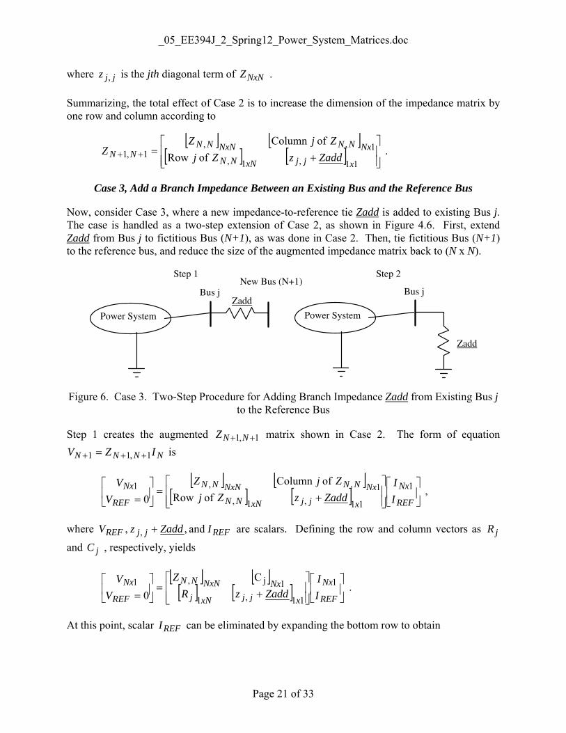
Consider the three-bus network shown in Figure that has five branch impedances and one current source.

1 2 3

ZE

ZA

ZB

ZC

ZDI3

Figure 1. Three-Bus Network

Applying KCL at the three independent nodes yields the following equations for the bus voltages (with respect to ground):

At bus 1, 0211 =−

+AE ZVV

ZV ,

At bus 2, 032122 =−

+−

+CAB ZVV

ZVV

ZV ,

At bus 3, 3233 I

ZVV

ZV

CD=

−+ .

Collecting terms and writing the equations in matrix form yields


of 33

⎥⎥⎥

⎦

⎤

⎢⎢⎢

⎣

⎡=

⎥⎥⎥

⎦

⎤

⎢⎢⎢

⎣

⎡

⎥⎥⎥⎥⎥⎥⎥

⎦

⎤

⎢⎢⎢⎢⎢⎢⎢

⎣

⎡

+−

−++−

−+

33

2

100

1110

11111

0111

IVVV

ZZZ

ZZZZZ

ZZZ

DCC

CCBAA

AAE

,

or in matrix form,

IYV = ,

where Y is the admittance matrix, V is a vector of bus voltages (with respect to ground), and I is a vector of current injections.

Voltage sources, if present, can be converted to current sources using the usual network rules. If a bus has a zero-impedance voltage source attached to it, then the bus voltage is already known, and the dimension of the problem is reduced by one.

A simple observation of the structure of the above admittance matrix leads to the following rule for building Y:

1. The diagonal terms of Y contain the sum of all branch admittances connected directly to the corresponding bus.

2. The off-diagonal elements of Y contain the negative sum of all branch admittances connected directly between the corresponding busses.

These rules make Y very simple to build using a computer program. For example, assume that the impedance data for the above network has the following form, one data input line per branch:

From To Branch Impedance (Entered Bus Bus as Complex Numbers)

1 0 ZE

1 2 ZA

2 0 ZB

2 3 ZC

3 0 ZD

The following FORTRAN instructions would automatically build Y, without the need of manually writing the KCL equations beforehand:

COMPLEX Y(3,3),ZB,YB

DATA Y/9 * 0.0/

1 READ(1,*,END=2) NF,NT,ZB


of 33

YB = 1.0 / ZB

C MODIFY THE DIAGONAL TERMS

IF(NF .NE. 0) Y(NF,NF) = Y(NF,NF) + YB

IF(NT .NE. 0) Y(NT,NT) = Y(NT,NT) + YB

IF(NF .NE. 0 .AND. NT .NE. 0) THEN

C MODIFY THE OFF-DIAGONAL TERMS

Y(NF,NT) = Y(NF,NT) - YB

Y(NT,NF) = Y(NT,NF) - YB

ENDIF

GO TO 1

2 STOP

END

Of course, error checking is needed in an actual computer program to detect data errors and dimension overruns. Also, if bus numbers are not compressed (i.e. bus 1 through bus N), then additional logic is needed to internally compress the busses, maintaining separate internal and external (i.e. user) bus numbers.

Note that the Y matrix is symmetric unless there are branches whose admittance is direction-dependent. In AC power system applications, only phase-shifting transformers have this asymmetric property. The normal 30o phase shift in wye-delta transformers creates asymmetry.

2. Gaussian Elimination and Backward Substitution

Gaussian elimination is the most common method for solving bus voltages in a circuit for which KCL equations have been written in the form

YVI = .

Of course, direct inversion can be used, where

IYV 1−= ,

but direct inversion for large matrices is computationally prohibitive or, at best, inefficient.

The objective of Gaussian elimination is to reduce the Y matrix to upper-right-triangular-plus-diagonal form (URT+D), then solve for V via backward substitution. A series of row operations (i.e. subtractions and additions) are used to change equation

⎥⎥⎥⎥⎥⎥

⎦

⎤

⎢⎢⎢⎢⎢⎢

⎣

⎡

⎥⎥⎥⎥⎥⎥

⎦

⎤

⎢⎢⎢⎢⎢⎢

⎣

⎡

=

⎥⎥⎥⎥⎥⎥

⎦

⎤

⎢⎢⎢⎢⎢⎢

⎣

⎡

NNNNNN

N

N

N

N V

VVV

yyyy

yyyyyyyyyyyy

I

III

M

L

MOMMM

L

L

L

M3

2

1

,3,2,1,

,33,32,31,3

,23,22,21,2

,13,12,11,1

3

2

1


of 33

into

⎥⎥⎥⎥⎥⎥

⎦

⎤

⎢⎢⎢⎢⎢⎢

⎣

⎡

⎥⎥⎥⎥⎥⎥

⎦

⎤

⎢⎢⎢⎢⎢⎢

⎣

⎡

=

⎥⎥⎥⎥⎥⎥

⎦

⎤

⎢⎢⎢⎢⎢⎢

⎣

⎡

NNN

N

N

N

N V

VVV

y

yyyyyyyyy

I

III

M

L

MOMMM

L

L

L

M3

2

1

,'

,3'

3,3'

,2'

3,2'

2,2'

,13,12,11,1

'

'3

'2

1

000

000

,

in which the transformed Y matrix has zeros under the diagonal.

For illustrative purposes, consider the two equations represented by Rows 1 and 2, which are

NN

NNVyVyVyVyIVyVyVyVyI

,233,222,211,22

,133,122,111,11++++=++++=

L

L .

Subtracting ( 1,1

1,2yy

• Row 1) from Row 2 yields

NNN

NN

Vyyy

yVyyy

yVyyy

yVyyy

yIyy

I

VyVyVyVyI

⎟⎟⎠

⎞⎜⎜⎝

⎛−++⎟

⎟⎠

⎞⎜⎜⎝

⎛−+⎟

⎟⎠

⎞⎜⎜⎝

⎛−+⎟

⎟⎠

⎞⎜⎜⎝

⎛−=−

++++=

,11,1

1,2,233,1

1,1

1,23,222,1

1,1

1,22,211,1

1,1

1,21,21

1,1

1,22

,133,122,111,11

L

L .

The coefficient of 1V in Row 2 is forced to zero, leaving Row 2 with the desired "reduced" form of

NNVyVyVyI ',23

'3,22

'2,2

'2 0 ++++= L .

Continuing, Row 1 is then used to "zero" the 1V coefficients in Rows 3 through N, one row at a time. Next, Row 2 is used to zero the 2V coefficients in Rows 3 through N, and so forth.

After the Gaussian elimination is completed, and the Y matrix is reduced to (URT+D) form, the bus voltages are solved by backward substitution as follows:

For Row N,

NNNN VyI ',

' = , so ( )''

,

1N

NNN I

yV = .

Next, for Row N-1,

NNNNNNN VyVyI ',11

'1,1

'1 −−−−− += , so ( )NNNN

NNN VyI

yV '

,1'

1'1,1

11

−−−−

− −= .


of 33

Continuing for Row j, where 2,,3,2 L−−= NNj ,

NNjjjjjjjj VyVyVyI ',1

'1,

',

' +++= ++ L , so

( )NNjjjjjjj

j VyVyIy

V ',1

'1,

'',

1−−−= ++ L ,

which, in general form, is described by

⎟⎟

⎠

⎞

⎜⎜

⎝

⎛−= ∑

+=kkj

N

jkj

jjj VyI

yV '

,1

'',

1 .

A simple FORTRAN computer program for solving V in an N-dimension problem using Gaussian elimination and backward substitution is given below.

COMPLEX Y(N,N),V(N),I(N),YMM

C GAUSSIAN ELIMINATE Y AND I

NM1 = N - 1

C PIVOT ON ROW M, M = 1,2,3, ... ,N-1

DO 1 M = 1,NM1

MP1 = M + 1

YMM = 1.0 / Y(M,M)

C OPERATE ON THE ROWS BELOW THE PIVOT ROW

DO 1 J = MP1,N

C THE JTH ROW OF I

I(J) = I(J) - Y(J,M) *YMM * I(M)

C THE JTH ROW OF Y, BELOW AND TO THE RIGHT OF THE PIVOT

C DIAGONAL

DO 1 K = M,N

Y(J,K) = Y(J,K) - Y(J,M) * YMM * Y(M,K)

1 CONTINUE

C BACKWARD SUBSTITUTE TO SOLVE FOR V

V(N) = I(N) / Y(N,N)

DO 2 M = 1,NM1

J = N - M

C BACKWARD SUBSTITUTE TO SOLVE FOR V, FOR

C ROW J = N-1,N-2,N-3, ... ,1

V(J) = I(J)

JP1 = J + 1

DO 3 K = JP1,N

V(J) = V(J) - Y(J,K) * V(K)


of 33

3 CONTINUE

V(J) = V(J) / Y(J,J)

2 CONTINUE

STOP

END

One disadvantage of Gaussian elimination is that if I changes, even though Y is fixed, the entire problem must be re-solved since the elimination of Y determines the row operations that must be repeated on I. Inversion and LU decomposition to not have this disadvantage.

3. Kron Reduction

Gaussian elimination can be made more computationally efficient by simply not performing operations whose results are already known. For example, instead of arithmetically forcing elements below the diagonal to zero, simply set them to zero at the appropriate times. Similarly, instead of dividing all elements below and to the right of a diagonal element by the diagonal element, divide only the elements in the diagonal row by the diagonal element, make the diagonal element unity, and the same effect will be achieved. This technique, which is actually a form of Gaussian elimination, is known as Kron reduction.

Kron reduction "pivots" on each diagonal element ',mmy , beginning with 1,1y , and continuing

through 1,1 −− NNy . Starting with Row m = 1, and continuing through Row m = N - 1, the algorithm for Kron reducing YVI = is

1. Divide the elements in Row m, that are to the right of the diagonal, by the diagonal element '

,mmy . (Note - the elements to the left of the diagonal are already zero).

2. Replace element 'mI with '

,

'

mm

m

y

I .

3. Replace diagonal element ',mmy with unity.

4. Modify the 'Y elements in rows greater than m and columns greater than m (i.e. below and to the right of the diagonal element) using

',

',

',

', kmmjkjkj yyyy −= , for j > m, k > m.

5. Modify the 'I elements below the mth row according to

'',

''mmjjj IyII −= , for j > m.

6. Zero the elements in Column m of 'Y that are below the diagonal element.


of 33

A FORTRAN code for Kron reduction is given below.

COMPLEX Y(N,N),V(N),I(N),YMM

C KRON REDUCE Y, WHILE ALSO PERFORMING ROW OPERATIONS ON I

NM1 = N - 1

C PIVOT ON ROW M, M = 1,2,3, ... ,N-1

DO 1 M = 1,NM1

MP1 = M + 1

YMM = 1.0 / YMM

C DIVIDE THE PIVOT ROW BY THE PIVOT

DO 2 K = MP1,N

Y(M,K) = Y(M,K) * YMM

2 CONTINUE

C OPERATE ON THE I VECTOR

I(M) = I(M) * YMM

C SET THE PIVOT TO UNITY

Y(M,M) = 1.0

C REDUCE THOSE ELEMENTS BELOW AND TO THE RIGHT OF THE PIVOT

DO 3 J = MP1,N

DO 4 K = MP1,N

Y(J,K) = Y(J,K) - Y(J,M) * Y(M,K)

4 CONTINUE

C OPERATE ON THE I VECTOR

I(J) = I(J) - Y(J,M) * I(M)

C SET THE Y ELEMENTS DIRECTLY BELOW THE PIVOT TO ZERO

Y(J,M) = 0.0

3 CONTINUE

1 CONTINUE

4. LU Decomposition

An efficient method for solving V in matrix equation YV = I is to decompose Y into the product of a lower-left-triangle-plus-diagonal (LLT+D) matrix L, and an (URT+D) matrix U, so that YV = I can be written as

LUV = I .

The benefits of decomposing Y will become obvious after observing the systematic procedure for finding V.

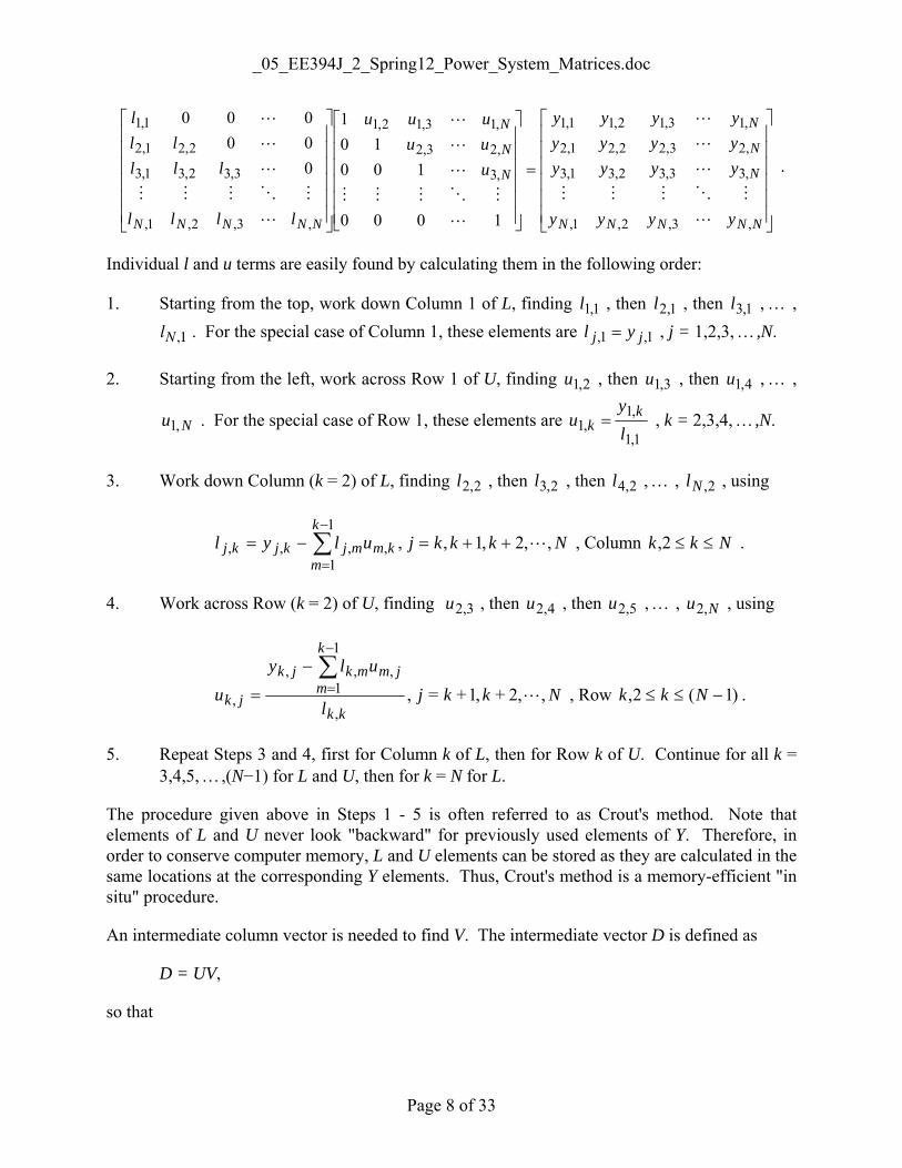
It is customary to set the diagonal terms of U equal to unity, so that there are a total of 2N unknown terms in L and U. LU = Y in expanded form is then


of 33

⎥⎥⎥⎥⎥⎥

⎦

⎤

⎢⎢⎢⎢⎢⎢

⎣

⎡

=

⎥⎥⎥⎥⎥⎥

⎦

⎤

⎢⎢⎢⎢⎢⎢

⎣

⎡

⎥⎥⎥⎥⎥⎥

⎦

⎤

⎢⎢⎢⎢⎢⎢

⎣

⎡

NNNNN

N

N

N

N

N

N

NNNNN yyyy

yyyyyyyyyyyy

uuuuuu

llll

lllll

l

,3,2,1,

,33,32,31,3

,23,22,21,2

,13,12,11,1

,3

,23,2

,13,12,1

,3,2,1,

3,32,31,3

2,21,2

1,1

1000

10010

1

000000

L

MOMMM

L

L

L

L

MOMMM

L

L

L

L

MOMMM

L

L

L

.

Individual l and u terms are easily found by calculating them in the following order:

1. Starting from the top, work down Column 1 of L, finding 1,1l , then 1,2l , then 1,3l , … , lN ,1 . For the special case of Column 1, these elements are 1,1, jj yl = , j = 1,2,3, …,N.

2. Starting from the left, work across Row 1 of U, finding 2,1u , then 3,1u , then 4,1u , … ,

Nu ,1 . For the special case of Row 1, these elements are 1,1

,1,1 l

yu k

k = , k = 2,3,4, …,N.

3. Work down Column (k = 2) of L, finding 2,2l , then 2,3l , then 2,4l , … , 2,Nl , using

Nkkkjulyl kmk

mmjkjkj ,,2,1, ,,

1

1,,, L++=−= ∑

−

= , Column Nkk ≤≤2, .

4. Work across Row (k = 2) of U, finding 3,2u , then 4,2u , then 5,2u , … , Nu ,2 , using

Nkkjl

ulyu

kk

k

mjmmkjk

jk ,,2+,1+= ,,

1

1,,,

, L

∑−

=−

= , Row )1(2, −≤≤ Nkk .

5. Repeat Steps 3 and 4, first for Column k of L, then for Row k of U. Continue for all k = 3,4,5, …,(N−1) for L and U, then for k = N for L.

The procedure given above in Steps 1 - 5 is often referred to as Crout's method. Note that elements of L and U never look "backward" for previously used elements of Y. Therefore, in order to conserve computer memory, L and U elements can be stored as they are calculated in the same locations at the corresponding Y elements. Thus, Crout's method is a memory-efficient "in situ" procedure.

An intermediate column vector is needed to find V. The intermediate vector D is defined as

D = UV,

so that


of 33

⎥⎥⎥⎥⎥⎥

⎦

⎤

⎢⎢⎢⎢⎢⎢

⎣

⎡

⎥⎥⎥⎥⎥⎥

⎦

⎤

⎢⎢⎢⎢⎢⎢

⎣

⎡

=

⎥⎥⎥⎥⎥⎥

⎦

⎤

⎢⎢⎢⎢⎢⎢

⎣

⎡

N

N

N

N

N V

VVV

uuuuuu

d

ddd

M

L

MOMMM

L

L

L

M3

2

1

,3

,23,2

,13,12,1

3

2

1

1000

10010

1

.

Since LUV = I, then LD = I. Vector D is found using forward-substitution from

⎥⎥⎥⎥⎥⎥

⎦

⎤

⎢⎢⎢⎢⎢⎢

⎣

⎡

=

⎥⎥⎥⎥⎥⎥

⎦

⎤

⎢⎢⎢⎢⎢⎢

⎣

⎡

⎥⎥⎥⎥⎥⎥

⎦

⎤

⎢⎢⎢⎢⎢⎢

⎣

⎡

NNNNNNN I

III

d

ddd

llll

lllll

l

MM

L

MOMMM

L

L

L

3

2

1

3

2

1

,3,2,1,

3,32,31,3

2,21,2

1,1

000000

,

which proceeds as follows:

From Row 1, ( )11,1

1111,11, I

ldIdl == ,

From Row 2, ( )11,222,2

2222,211,21 , dlI

ldIdldl −==+ ,

From Row k, ⎟⎟

⎠

⎞

⎜⎜

⎝

⎛−==+++ ∑

−

=jjk

k

jk

kkkkkkkkk dlI

ldIdldldl ,

1

1,,22,11,

1, L .

Now, since D = UV, or

⎥⎥⎥⎥⎥⎥

⎦

⎤

⎢⎢⎢⎢⎢⎢

⎣

⎡

⎥⎥⎥⎥⎥⎥

⎦

⎤

⎢⎢⎢⎢⎢⎢

⎣

⎡

=

⎥⎥⎥⎥⎥⎥

⎦

⎤

⎢⎢⎢⎢⎢⎢

⎣

⎡

N

N

N

N

N V

VVV

uuuuuu

d

ddd

M

L

MOMMM

L

L

L

M3

2

1

,3

,23,2

,13,12,1

3

2

1

1000

10010

1

,

where D and U are known, then V is found using backward substitution.

An important advantage of LU decomposition over Gaussian elimination or Kron reduction is that the I vector is not modified during decomposition. Therefore, once Y has been decomposed into L and U, I can be modified, and V recalculated, with minimal work, using the forward and backward substitution steps shown above.


of 33

A special form of L is helpful when Y is symmetric. In that case, let both L and U have unity diagonal terms, and define a diagonal matrix D so that

Y = LDU ,

or

⎥⎥⎥⎥⎥⎥

⎦

⎤

⎢⎢⎢⎢⎢⎢

⎣

⎡

⎥⎥⎥⎥⎥⎥

⎦

⎤

⎢⎢⎢⎢⎢⎢

⎣

⎡

⎥⎥⎥⎥⎥⎥

⎦

⎤

⎢⎢⎢⎢⎢⎢

⎣

⎡

=

1000

10010

1

000

000000000

10010010001

,3

,23,2

,13,12,1

,

3,3

2,2

1,1

3,2,1,

2,31,3

1,2

L

MOMMM

L

L

L

L

MOMMM

L

L

L

L

OMMM

L

L

L

N

N

N

NNNNN

uuuuuu

d

dd

d

lll

lll

Y .

Since Y is symmetric, then TYY = , and [ ] TTTTTT DLULDULDULDU === . Therefore,

an acceptable solution is to allow TUL = . Incorporating this into the above equation yields

⎥⎥⎥⎥⎥⎥

⎦

⎤

⎢⎢⎢⎢⎢⎢

⎣

⎡

⎥⎥⎥⎥⎥⎥

⎦

⎤

⎢⎢⎢⎢⎢⎢

⎣

⎡

=

NN

N

N

N

NNN d

lddldlddldldldd

lll

lll

Y

,

3,3,33,3

2,2,22,32,22,2

1,1,11,31,11,21,11,1

3,2,1,

2,31,3

1,2

000

000

10010010001

L

MOMMM

L

L

L

L

OMMM

L

L

L

,

which can be solved by working from top-to-bottom, beginning with Column 1 of Y, as follows:

Working down Column 1 of Y,

1,11,1 dy = ,

1,11,21,21,11,21,2 / so , dyldly == ,

1,11,1,1,11,1, / so , dyldly jjjj == .

Working down Column 2 of Y,

1,21,11,22,22,22,21,21,11,22,2 so , ldlyddldly −=+= ,

( ) Njdldlyldlldly jjjjjj ≤<−=+= 2 ,/ so , 2,21,21,11,2,2,2,22,1,21,11,2, .

Working down Column k of Y,


of 33

mkmmk

mmkkkkkkkmkmm

k

mmkkk ldlyddldly ,,

1

1,,,,,,

1

1,, so , ∑∑

−

=

−

=−=+= ,

Njkdldlylldly kkmkmmk

mmjkjkjmkmm

k

mmjkj ≤<⎟

⎟⎠

⎞⎜⎜⎝

⎛−== ∑∑

−

=

−

= ,/ so , ,,,

1

1,,,,,

1

1,, .

This simplification reduces memory and computation requirements for LU decomposition by approximately one-half.

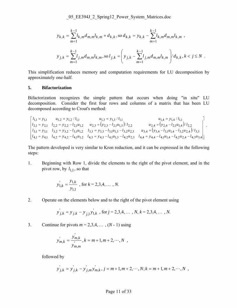
5. Bifactorization

Bifactorization recognizes the simple pattern that occurs when doing "in situ" LU decomposition. Consider the first four rows and columns of a matrix that has been LU decomposed according to Crout's method:

( ) ( )( )

⎥⎥⎥⎥⎥

⎦

⎤

⎢⎢⎢⎢⎢

⎣

⎡

−−−=−−=−==−−=−−=−==

−=−=−======

4,33,44,22,44,11,44,44,43,22,43,11,43,43,42,11,42,42,41,41,4

3,34,22,34,11,34,34,33,22,33,11,33,33,32,11,32,32,31,31,3

2,24,11,24,24,22,23,11,23,23,22,11,22,22,21,21,2

1,14,14,11,13,13,11,12,12,11,11,1

///

///

ulululylululylulylyllululyuululylulylyl

lulyululyuulylyllyulyulyuyl

.

The pattern developed is very similar to Kron reduction, and it can be expressed in the following steps:

1. Beginning with Row 1, divide the elements to the right of the pivot element, and in the pivot row, by 1,1l , so that

1,1

,1',1 y

yy k

k = , for k = 2,3,4, … , N.

2. Operate on the elements below and to the right of the pivot element using

',11,,

', kjkjkj yyyy −= , for j = 2,3,4, … , N, k = 2,3,4, … , N.

3. Continue for pivots m = 2,3,4, … , (N - 1) using

Nmmky

yy

mm

kmkm ,,2,1,

',

','

, L++== ,

followed by

NmmkNmmjyyyy kmmjkjkj ,,2,1;,,2,1,',

',

',

', LL ++=++=−= ,


of 33

for each pivot m.

When completed, matrix Y' has been replaced by matrices L and U as follows:

⎥⎥⎥⎥⎥⎥

⎦

⎤

⎢⎢⎢⎢⎢⎢

⎣

⎡

=

NNNNN llll

ullluulluuul

Y

,3,2,1,

5,33,32,31,3

5,23,22,21,2

5,13,12,11,1

'

L

OMMM

L

L

L

,

and where the diagonal u elements are unity (i.e. 1 ,3,32,21,1 ===== NNuuuu L ).

The corresponding FORTRAN code for bifactorization is

COMPLEX Y(N,N),YMM

C DO FOR EACH PIVOT M = 1,2,3, ... ,N - 1

NM1 = N - 1

DO 1 M = 1,NM1

C FOR THE PIVOT ROW

MP1 = M + 1

YMM = 1.0 / Y(M,M)

DO 2 K = MP1,N

Y(M,K) = Y(M,K) * YMM

2 CONTINUE

C BELOW AND TO THE RIGHT OF THE PIVOT ELEMENT

DO 3 J = MP1,N

DO 3 K = MP1,N

Y(J,K) = Y(J,K) - Y(J,M) * Y(M,K)

3 CONTINUE

1 CONTINUE

STOP

END

6. Shipley-Coleman Inversion

For relatively small matrices, it is possible to obtain the inverse directly. The Shipley-Coleman inversion method for inversion is popular because it is easily programmed. The algorithm is

1. For each pivot (i.e. diagonal term) m, m = 1,2,3, … ,N, perform the following Steps 2 - 4.

2. Kron reduce all elements in Y, above and below, except those in Column m and Row m using


of 33

mkNkmjNjy

yyyy

mm

kmmjkjkj ≠=≠=−= ,,,3,2,1 ; ,,,3,2,1 ,

,

',

','

,', LL .

3. Replace pivot element ',mmy with its negative inverse, i.e.

',

1

mmy− .

4. Multiply all elements in Row m and Column m, except the pivot, by ',mmy .

The result of this procedure is actually the negative inverse, so that when completed, all terms must be negated. A FORTRAN code for Shipley-Coleman is shown below.

COMPLEX Y(N,N),YPIV

C DO FOR EACH PIVOT M = 1,2,3, ... ,N

DO 1 M = 1,N

YPIV = 1.0 / Y(M,M)

C KRON REDUCE ALL ROWS AND COLUMNS, EXCEPT THE PIVOT ROW

C AND PIVOT COLUMN

DO 2 J = 1,N

IF(J .EQ. M) GO TO 2

DO 2 K = 1,N

IF(K. NE. M) Y(J,K) = Y(J,K) - Y(J,M) * Y(M,K) * YPIV

2 CONTINUE

C REPLACE THE PIVOT WITH ITS NEGATIVE INVERSE

YPIV = -YPIV

Y(M,M) = YPIV

C WORK ACROSS THE PIVOT ROW AND DOWN THE PIVOT COLUMN,

C MULTIPLYING BY THE NEW PIVOT VALUE

DO 3 K = 1,N

IF(K .EQ. M) GO TO 3

Y(M,K) = Y(M,K) * YPIV

Y(K,M) = Y(K,M) * YPIV

3 CONTINUE

1 CONTINUE

C NEGATE THE RESULTS

DO 4 J = 1,N

DO 4 K = 1,N

Y(J,K) = -Y(J,K)

4 CONTINUE

STOP

END


of 33

The order of the number of calculations for Shipley-Coleman is 3N .

7. Impedance Matrix

The impedance matrix is the inverse of the admittance matrix, or

1−= YZ ,

so that

ZIV = .

The reference bus both Y and Z is ground. Although the impedance matrix can be found via inversion, complete inversion is not common for matrices with more than a few hundred rows and columns because of the matrix storage requirements. In those instances, Z elements are usually found via Gaussian elimination, Kron reduction, or, less commonly, by a direct building algorithm. If only a few of the Z elements are needed, then Gaussian elimination or Kron reduction are best. Both methods are described in following sections.

8. Physical Significance of Admittance and Impedance Matrices

The physical significance of the admittance and impedance matrices can be seen by examining the basic matrix equations YVI = and ZIIYV == −1 . Expanding the jth row of YVI = yields

∑=

=N

kkkjj VyI

1, . Therefore,

kmNmmVk

jkj V

Iy

≠==

=,,,2,1,0

,L

,

where, as shown in Figure 2, all busses except k are grounded, kV is a voltage source attached to bus k, and jI is the resulting current injection at (i.e. flowing into) bus j. Since all busses that

neighbor bus k are grounded, the currents induced by kV will not get past these neighbors, and the only non-zero injection currents jI will occur at the neighboring busses. In a large power system, most busses do not neighbor any arbitrary bus k. Therefore, Y consists mainly of zeros (i.e. is sparse) in most power systems.


of 33

+

-Vk

Bus jApplied Voltage

Power System

Ij

All Other BussesGrounded

at Bus k

Induced Current at

A

Figure 2. Measurement of Admittance Matrix Term kjy ,

Concerning Z, the kth row of ZIIYV == −1 yields ∑=

=N

jjjkk IzV

1, . Hence,

kmNmmIk

jkj I

Vz

≠==

=,,,2,1,0

,L

,

where, as shown in Figure 3, Ik is a current source attached to bus k, Vj is the resulting voltage at bus j, and all busses except k are open-circuited. Unless the network is disjoint, then current injection at one bus, when all other busses open-circuited, will raise the potential everywhere in the network. For that reason, Z tends to be full.

Power System

All Other BussesOpen Circuited

Applied Current atInduced Voltage

+

-V

Bus kat Bus j

IkVj

Figure 3. Measurement of Impedance Matrix Term kjz ,

9. Formation of the Impedance Matrix via Gaussian Elimination, Kron Reduction, and LU Decomposition

Gaussian Elimination

An efficient method of fully or partially inverting a matrix is to formulate the problem using Gaussian elimination. For example, given


of 33

IYZ = ,

where Y is a matrix of numbers, Z is a matrix of unknowns, and I is the identity matrix, the objective is to Gaussian eliminate Y, while performing the same row operations on I, to obtain the form

IZY ′=′ ,

where Y' is in (URT+D) form. Then, individual columns of Z can then be solved using backward substitution, one at a time. This procedure is also known as the augmentation method, and it is illustrated as follows:

Y is first Gaussian eliminated, as shown in a previous section, while at the same time performing identical row operations on I. Afterward, the form of IZY ′=′ is

=

⎥⎥⎥⎥⎥⎥

⎦

⎤

⎢⎢⎢⎢⎢⎢

⎣

⎡

⎥⎥⎥⎥⎥⎥

⎦

⎤

⎢⎢⎢⎢⎢⎢

⎣

⎡

NNNNN

N

N

N

NN

N

N

N

zzzz

zzzzzzzzzzzz

y

yyyyyyyyy

,3,2,1,

,33,32,31,3

,23,22,21,2

,13,12,11,1

,'

,3'

3,3'

,2'

3,2'

2,2'

,13,12,11,1

000

000

L

MOMMM

L

L

L

L

MOMMM

L

L

L

⎥⎥⎥⎥⎥⎥

⎦

⎤

⎢⎢⎢⎢⎢⎢

⎣

⎡

',

'3,

'2,

'1,

'3,3

'2,3

'1,3

'2,2

'1,2

0000001

NNNNN IIII

IIIII

L

MOMMM

L

L

L

where Rows 1 of Y' and I' are the same as in Y and I. The above equation can be written in abbreviated column form as

[ ] [ ]''3

'2

'1321

,'

,3'

3,3'

,2'

3,2'

2,2'

,13,12,11,1

000

000

NN

NN

N

N

N

IIIIZZZZ

y

yyyyyyyyy

LL

L

MOMMM

L

L

L

=

⎥⎥⎥⎥⎥⎥

⎦

⎤

⎢⎢⎢⎢⎢⎢

⎣

⎡

,

where the individual column vectors Zi and Ii have dimension N x 1. The above equation can be solved as N separate subproblems, where each subproblem computes a column of Z. For example, the kth column of Z can be computed by applying backward substitution to


of 33

⎥⎥⎥⎥⎥⎥⎥

⎦

⎤

⎢⎢⎢⎢⎢⎢⎢

⎣

⎡

=

⎥⎥⎥⎥⎥⎥

⎦

⎤

⎢⎢⎢⎢⎢⎢

⎣

⎡

⎥⎥⎥⎥⎥⎥

⎦

⎤

⎢⎢⎢⎢⎢⎢

⎣

⎡

',

',3

',2

',1

,

,3

,2

,1

,'

,3'

3,3'

,2'

3,2'

2,2'

,13,12,11,1

000

000

kN

k

k

k

kN

k

k

k

NN

N

N

N

I

III

Z

ZZZ

y

yyyyyyyyy

MM

L

MOMMM

L

L

L

.

Each column of Z is solved independently from the others.

Kron Reduction

If Kron reduction, the problem is essentially the same, except that Row 1 of the above equation is divided by '

1,1y , yielding

⎥⎥⎥⎥⎥⎥⎥

⎦

⎤

⎢⎢⎢⎢⎢⎢⎢

⎣

⎡

=

⎥⎥⎥⎥⎥⎥

⎦

⎤

⎢⎢⎢⎢⎢⎢

⎣

⎡

⎥⎥⎥⎥⎥⎥

⎦

⎤

⎢⎢⎢⎢⎢⎢

⎣

⎡

',

',3

',2

',1

,

,3

,2

,1

,'

,3'

3,3'

,2'

3,2'

2,2'

,13,12,11,1

000

000

kN

k

k

k

kN

k

k

k

NN

N

N

N

I

III

Z

ZZZ

y

yyyyyyyyy

MM

L

MOMMM

L

L

L

.

Because backward substitution can stop when the last desired z element is computed, the process is most efficient if the busses are ordered so that the highest bus numbers (i.e. N, N-1, N-2, etc.) correspond to the desired z elements. Busses can be ordered accordingly when forming Y to take advantage of this efficiency.

LU Decomposition

Concerning LU decomposition, once the Y matrix has been decomposed into L and U, then we have

ILUZYZ == ,

where I is the identity matrix. Expanding the above equation as [ ] IUZL = yields

=

⎥⎥⎥⎥⎥⎥

⎦

⎤

⎢⎢⎢⎢⎢⎢

⎣

⎡

⎥⎥⎥⎥⎥⎥

⎦

⎤

⎢⎢⎢⎢⎢⎢

⎣

⎡

NNNNN

N

N

N

NNNNN uzuzuzuz

uzuzuzuzuzuzuzuzuzuzuzuz

llll

lllll

l

,3,2,1,

,33,32,31,3

,23,22,21,2

,13,12,11,1

,3,2,1,

3,33,21,3

2,21,2

1,1

000000

L

MOMMM

L

L

L

L

MOMMM

L

L

L

.


of 33

⎥⎥⎥⎥⎥⎥

⎦

⎤

⎢⎢⎢⎢⎢⎢

⎣

⎡

1000

010000100001

L

MOMMM

L

L

L

The special structure of the above equation shows that, in general, UZ must be (LLT+D) in form. UZ can be found by using forward substitution on the above equation, and then Z can be found, one column at a time, by using backward substitution on [ ][ ]ZUUZ = , which in expanded form is

=

⎥⎥⎥⎥⎥⎥

⎦

⎤

⎢⎢⎢⎢⎢⎢

⎣

⎡

⎥⎥⎥⎥⎥⎥

⎦

⎤

⎢⎢⎢⎢⎢⎢

⎣

⎡

NNNNN

N

N

N

N

N

N

zzzz

zzzzzzzzzzzz

uuuuuu

,3,2,1,

,33,32,31,3

,23,22,21,2

,13,12,11,1

,3

,23,2

,13,12,1

1000

10010

1

L

MOMMM

L

L

L

L

MOMMM

L

L

L

⎥⎥⎥⎥⎥⎥

⎦

⎤

⎢⎢⎢⎢⎢⎢

⎣

⎡

NNNNN uzuzuzuz

uzuzuzuzuz

uz

,3,2,1,

3,32,31,3

2,21,2

1,1

000000

L

MOMMM

L

L

L

.

10. Direct Impedance Matrix Building and Modification Algorithm

The impedance matrix can be built directly without need of the admittance matrix, if the physical properties of Z are exploited. Furthermore, once Z has been built, no matter which method was used, it can be easily modified when network changes occur. This after-the-fact modification capability is the most important feature of the direct impedance matrix building and modification algorithm.

The four cases to be considered in the algorithm are

Case 1. Add a branch impedance between a new bus and the reference bus.

Case 2. Add a branch impedance between a new bus and an existing non-reference bus.

Case 3. Add a branch impedance between an existing bus and the reference bus.

Case 4. Add a branch impedance between two existing non-reference busses.

Direct formation of an impedance matrix, plus all network modifications, can be achieved through these four cases. Each of the four is now considered separately.


of 33

Case 1, Add a Branch Impedance Between a New Bus and the Reference Bus

Case 1 is applicable in two situations. First, it is the starting point when building a new impedance matrix. Second, it provides (as does Case 2) a method for adding new busses to an existing impedance matrix.

Both situations applicable to Case 1 are shown in Figure 4. The starting-point situation is on the left, and the new-bus situation is on the right.

Power SystemN Busses

Zadd

Bus 1

ReferenceBus

Zadd

Bus (N+1)

Situation 1 Situation 2

ReferenceBus

Figure 4. Case 1, Add a Branch Impedance Between a New Bus and the Reference Bus

The impedance matrices for the two situations are

Situation 1 ZaddZ =1,1 ,

Situation 2: [ ]

[ ] [ ] ⎥⎥⎥⎥⎥⎥

⎦

⎤

⎢⎢⎢⎢⎢⎢

⎣

⎡

⎥⎥⎥⎥

⎦

⎤

⎢⎢⎢⎢

⎣

⎡

=++

1111

,1,1

0000

00

xxNNx

NxNNNNN

Zadd

ZZ

L

M .

The effect of situation 2 is simply to augment the existing NNZ , by a column of zeros, a row of zeros, and a new diagonal element Zadd. New bus (N+1) is isolated from the rest of the system.

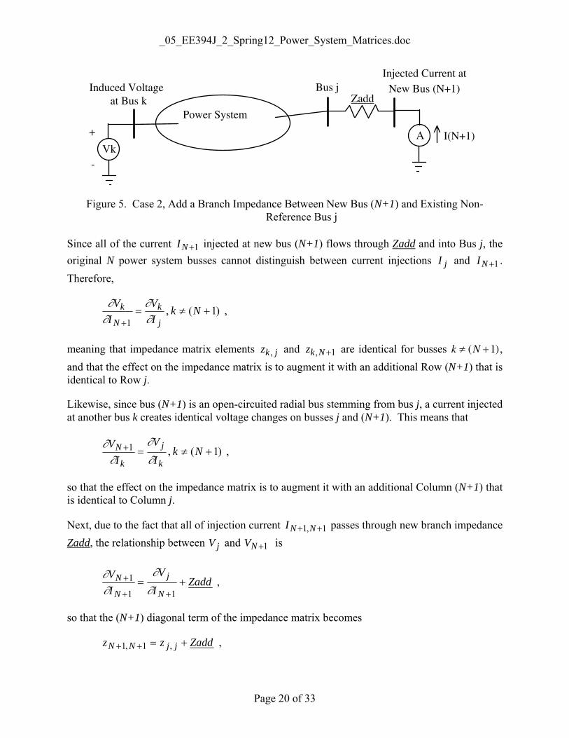
Case 2, Add a Branch Impedance Between a New Bus and an Existing Non-Reference Bus

Consider Case 2, shown in Figure 5, where a branch impedance Zadd is added from existing non-reference bus j to new bus (N+1). Before the addition, the power system has N busses, plus a reference bus (which is normally ground), and an impedance matrix NNZ , .


of 33

+

-Vk

Bus j

Power Systemat Bus k

A

Induced VoltageInjected Current at

I(N+1)

ZaddNew Bus (N+1)

Figure 5. Case 2, Add a Branch Impedance Between New Bus (N+1) and Existing Non-Reference Bus j

Since all of the current 1+NI injected at new bus (N+1) flows through Zadd and into Bus j, the original N power system busses cannot distinguish between current injections jI and 1+NI . Therefore,

)1( ,1

+≠=+

NkIV

IV

j

k

N

k∂∂

∂∂

,

meaning that impedance matrix elements jkz , and 1, +Nkz are identical for busses k N≠ +( )1 , and that the effect on the impedance matrix is to augment it with an additional Row (N+1) that is identical to Row j.

Likewise, since bus (N+1) is an open-circuited radial bus stemming from bus j, a current injected at another bus k creates identical voltage changes on busses j and (N+1). This means that

)1( ,1 +≠=+ NkIV

IV

k

j

k

N∂

∂

∂∂

,

so that the effect on the impedance matrix is to augment it with an additional Column (N+1) that is identical to Column j.

Next, due to the fact that all of injection current 1,1 ++ NNI passes through new branch impedance Zadd, the relationship between jV and 1+NV is

ZaddIV

IV

N

j

N

N +=++

+

11

1∂∂

∂∂

,

so that the (N+1) diagonal term of the impedance matrix becomes

Zaddzz jjNN +=++ ,1,1 ,


of 33

where jjz , is the jth diagonal term of NxNZ .

Summarizing, the total effect of Case 2 is to increase the dimension of the impedance matrix by one row and column according to

[ ] [ ]

[ ] [ ] ⎥⎥⎦

⎤

⎢⎢⎣

⎡+=++

11,1,1,,

1,1 of Row of Column

xjjxNNNNxNNNxNNN

NN ZaddzZjZjZ

Z .

Case 3, Add a Branch Impedance Between an Existing Bus and the Reference Bus

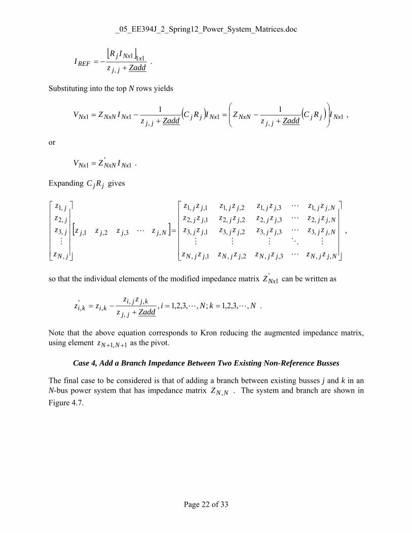
Now, consider Case 3, where a new impedance-to-reference tie Zadd is added to existing Bus j. The case is handled as a two-step extension of Case 2, as shown in Figure 4.6. First, extend Zadd from Bus j to fictitious Bus (N+1), as was done in Case 2. Then, tie fictitious Bus (N+1) to the reference bus, and reduce the size of the augmented impedance matrix back to (N x N).

Bus j

Power System

New Bus (N+1)Step 1 Step 2

Bus j

Power System

Zadd

Zadd

Figure 6. Case 3. Two-Step Procedure for Adding Branch Impedance Zadd from Existing Bus j to the Reference Bus

Step 1 creates the augmented 1,1 ++ NNZ matrix shown in Case 2. The form of equation

NNNN IZV 1,11 +++ = is

[ ] [ ]

[ ] [ ] ⎥⎦

⎤⎢⎣

⎡

⎥⎥⎦

⎤

⎢⎢⎣

⎡+=⎥

⎦

⎤⎢⎣

⎡= REF

Nx

xjjxNNNNxNNNxNNN

REF

NxII

ZaddzZjZjZ

VV 1

11,1,1,,1

of Row of Column

0 ,

where REFjjREF IZaddzV and , , , + are scalars. Defining the row and column vectors as jR

and jC , respectively, yields

[ ] [ ][ ] [ ] ⎥

⎦

⎤⎢⎣

⎡

⎥⎥⎦

⎤

⎢⎢⎣

⎡+=⎥

⎦

⎤⎢⎣

⎡= REF

Nx

xjjxNjNxNxNNN

REF

NxII

ZaddzRZ

VV 1

11,1

1j,1 C

0 .

At this point, scalar REFI can be eliminated by expanding the bottom row to obtain


of 33

[ ]

Zaddz

IRI

jj

xNxjREF +

−=,

111 .

Substituting into the top N rows yields

( ) ( ) 1,

1,

111 1 Nxjj

jjNxNNxjj

jjNxNxNNx IRC

ZaddzZIRC

ZaddzIZV ⎟

⎟⎠

⎞⎜⎜⎝

⎛

+−=

+−= ,

or

1'

1 NxNxNNx IZV = .

Expanding jjRC gives

[ ]

⎥⎥⎥⎥⎥⎥

⎦

⎤

⎢⎢⎢⎢⎢⎢

⎣

⎡

=

⎥⎥⎥⎥⎥⎥

⎦

⎤

⎢⎢⎢⎢⎢⎢

⎣

⎡

NjjNjjNjjNjjN

Njjjjjjjj

Njjjjjjjj

Njjjjjjjj

Njjjj

jN

j

j

j

zzzzzzzz

zzzzzzzzzzzzzzzzzzzzzzzz

zzzz

z

zzz

,,3,,2,,1,,

,,33,,32,,31,,3

,,23,,22,,21,,2

,,13,,12,,11,,1

,3,2,1,

,

,3

,2

,1

L

MOMMM

L

L

L

L

M

,

so that the individual elements of the modified impedance matrix '1NxZ can be written as

NkNiZaddz

zzzz

jj

kjjikiki ,,3,2,1 ;,,3,2,1 ,

,

,,,

', LL ==

+−= .

Note that the above equation corresponds to Kron reducing the augmented impedance matrix, using element 1,1 ++ NNz as the pivot.

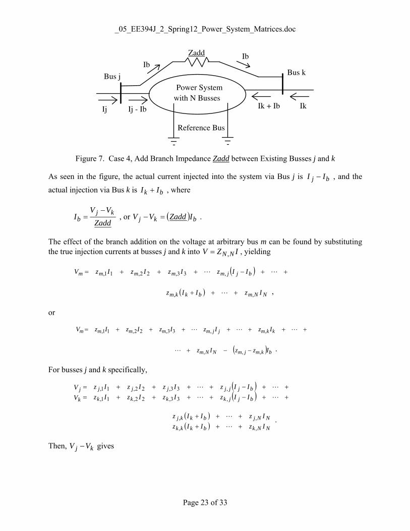
Case 4, Add a Branch Impedance Between Two Existing Non-Reference Busses

The final case to be considered is that of adding a branch between existing busses j and k in an N-bus power system that has impedance matrix NNZ , . The system and branch are shown in Figure 4.7.


of 33

Power System

Zadd

Reference Bus

Bus j

Ij

Ib

Ij - Ib

Bus k

IkIk + Ib

Ib

with N Busses

Figure 7. Case 4, Add Branch Impedance Zadd between Existing Busses j and k

As seen in the figure, the actual current injected into the system via Bus j is bj II − , and the

actual injection via Bus k is bk II + , where

Zadd

VVI kjb

−= , or ( ) bkj IZaddVV =− .

The effect of the branch addition on the voltage at arbitrary bus m can be found by substituting the true injection currents at busses j and k into IZV NN ,= , yielding

( ) ++−+++= LL bjjmmmmm IIzIzIzIzV ,33,22,11,

( ) NNmbkkm IzIIz ,, +++ L ,

or

+++++++= LLL kkmjjmmmmm IzIzIzIzIzV ,,33,22,11,

( ) bkmjmNNm IzzIz ,,, −−+L .

For busses j and k specifically,

( )( ) ++−++++=

++−++++=LL

LL

bjjkkkk

bjjjjjj

k

jIIzIzIzIzIIzIzIzIz

VV

,33,22,11,

,33,22,11,

( )( ) NNkbkkk

NNjbkkjIzIIzIzIIz

,,

,,++++++

L

L .

Then, kj VV − gives


of 33

( ) ( ) ( ) ( )( ) LL ,,33,3,22,2,11,1, +−−++−+−+−=− bjjkjjkjkjkjkj IIzzIzzIzzIzzVV

( )( ) ( ) NNkNjbkkkkj IzzIIzz ,,,, −+++− L .

Substituting in ( ) bkj IZaddVV =− and combining terms then yields

( ) ( ) ( ) ( ) LL 0 ,,33,3,22,2,11,1, +−++−+−+−= jjkjjkjkjkj IzzIzzIzzIzz

( ) ( ) ( ) bjkkjkkjjNNkNjkkkkj IZaddzzzzIzzIzz +−−+−−++− ,,,,,,,, L .

All of the above effects can be included as an additional row and column in equation IZV NN ,= as follows:

[ ][ ]

[ ] [ ][ ] [ ] ⎥

⎥⎦

⎤

⎢⎢⎣

⎡+−−+−

−=⎥

⎦

⎤⎢⎣

⎡

1,,,,1,,1,,,

1

1 f R f Row

f Col f Col0 NxjkkjkkjjxNNNNN

NxNNNNNxNNN

Nx

NxNZaddzzzzZokowZoj

ZokZojZV .

[ ][ ] ⎥

⎦

⎤⎢⎣

⎡− 11

1

xb

NxNI

I.

As was done in Case 3, the effect of the augmented row and column of the above equation can be incorporated into a modified impedance matrix by using Kron reduction, where element zN N+ +1 1, is the pivot, yielding

( )( )

Zaddzzzzzzzz

zzjkkjkkjj

mkmjkijimimi +−−+

−−−=

,,,,

,,,,,

', .

Application Notes

Once an impedance matrix is built, no matter which method is used, the modification algorithm can very easily adjust Z for network changes. For example, a branch outage can be effectively achieved by placing an impedance, of the same but negative value, in parallel with the actual impedance, so that the impedance of the parallel combination is infinite.

11. Example Code YZBUILD for Building Admittance Matrix and Impedance Matrix c c program yzbuild. 10/10/04. c implicit none complex ybus,yline,ycap,ctap,yii,ykk,yik,yki complex lmat,umat,unity,czero,ytest,ysave,diff,uz, 1 uzelem,zbus,elem,alpha integer nb,nbus,nfrom,nto,j,k,ipiv,jdum,kdum,jm1,kp1,l integer nlu,ipiv1,nm1,ny,nbext,nbint,iout,mxext,mxint integer jp1,ipp1,ngy,ngu real eps4,eps6,eps9,pi,dr,qshunt,r,x,charge,fill,ymag,umag


of 33

dimension ybus(150,150),nbext(150),nbint(9999) dimension lmat(150,150),umat(150,150),ysave(150,150), 1 uz(150,150),zbus(150,150),unity(150,150) data mxint/150/,mxext/9999/,nbus/0/, nbint/9999 * 0/, iout/6/, 1 nbext/150 * 0/,czero /(0.0,0.0)/,eps4/1.0e-04/, 2 eps6/1.0e-06/,eps9/1.0e-09/ data ybus /22500 * (0.0,0.0)/ data zbus /22500 * (0.0,0.0)/ data uz /22500 * (0.0,0.0)/ data unity /22500 * (0.0,0.0)/ c pi = 4.0 * atan(1.0) dr = 180.0 / pi open(unit=1,file='uz.txt') write(1,*) 'errors' close(unit=1,status='keep') open(unit=1,file='zbus_from_lu.txt') write(1,*) 'errors' close(unit=1,status='keep') open(unit=1,file='ybus_gaussian_eliminated.txt') write(1,*) 'errors' close(unit=1,status='keep') open(unit=1,file='unity_mat.txt') write(1,*) 'errors' close(unit=1,status='keep') open(unit=1,file='zbus_from_gaussian_elim.txt') write(1,*) 'errors' close(unit=1,status='keep') open(unit=6,file='yzbuild_screen_output.txt') open(unit=2,file='ybus.txt') open(unit=1,file='bdat.csv') write(6,*) 'program yzbuild, 150 bus version, 10/10/04' write(2,*) 'program yzbuild, 150 bus version, 10/10/04' write(6,*) 'read bus data from file bdat.csv' write(6,*) 'number b' write(2,*) 'read bus data from file bdat.csv' write(2,*) 'number b' c c read the bdat.csv file c 1 read(1,*,end=5,err=30) nb,qshunt if(nb .eq. 0) go to 5 write(6,1002) nb,qshunt write(2,1002) nb,qshunt 1002 format(i7,5x,f10.4) if(nb .le. 0 .or. nb .gt. mxext) then write(6,*) 'illegal bus number - stop' write(2,*) 'illegal bus number - stop' write(*,*) 'illegal bus number - stop' stop endif nbus = nbus + 1 if(nbus .gt. mxint) then write(6,*) 'too many busses - stop' write(2,*) 'too many busses - stop' write(*,*) 'too many busses - stop' stop


of 33

endif nbext(nbus) = nb nbint(nb) = nbus ycap = cmplx(0.0,qshunt) ybus(nbus,nbus) = ybus(nbus,nbus) + ycap go to 1 5 close(unit=1,status='keep') c open(unit=1,file='ldat.csv') write(6,*) write(6,*) 'read line/transformer data from file ldat.csv' write(6,*) ' from to r x', 1 ' b' write(2,*) 'read line/transformer data from file ldat.csv' write(2,*) ' from to r x', 1 ' b' c c read the ldat.csv file c 10 read(1,*,end=15,err=31) nfrom,nto,r,x,charge if(nfrom .eq. 0 .and. nto .eq. 0) go to 15 write(6,1004) nfrom,nto,r,x,charge write(2,1004) nfrom,nto,r,x,charge 1004 format(1x,i5,2x,i5,3(2x,f10.4)) if(nfrom .lt. 0 .or. nfrom .gt. mxext .or. nto .lt. 0 1 .or. nto .gt. mxext) then write(6,*) 'illegal bus number - stop' write(2,*) 'illegal bus number - stop' write(*,*) 'illegal bus number - stop' stop endif if(nfrom .eq. nto) then write(6,*) 'same bus number given on both ends - stop' write(2,*) 'same bus number given on both ends - stop' write(*,*) 'same bus number given on both ends - stop' stop endif if(r .lt. -eps6) then write(6,*) 'illegal resistance - stop' write(2,*) 'illegal resistance - stop' write(*,*) 'illegal resistance - stop' stop endif if(charge .lt. -eps6) then write(6,*) 'line charging should be positive' write(2,*) 'line charging should be positive' write(*,*) 'line charging should be positive' stop endif if(nfrom .ne. 0) then nfrom = nbint(nfrom) if(nfrom .eq. 0) then write(6,*) 'bus not included in file bdat.csv - stop' write(2,*) 'bus not included in file bdat.csv - stop' write(*,*) 'bus not included in file bdat.csv - stop' stop endif endif if(nto .ne. 0) then nto = nbint(nto)


of 33

if(nto .eq. 0) then write(6,*) 'bus not included in file bdat.csv - stop' write(2,*) 'bus not included in file bdat.csv - stop' write(*,*) 'bus not included in file bdat.csv - stop' stop endif endif yline = cmplx(r,x) if(cabs(yline) .lt. eps6) go to 10 yline = 1.0 / yline ycap = cmplx(0.0,charge / 2.0) c c the line charging terms c if(nfrom .ne. 0) ybus(nfrom,nfrom) = ybus(nfrom,nfrom) + ycap if(nto .ne. 0) ybus(nto ,nto ) = ybus(nto ,nto ) + ycap c c shunt elements c if(nfrom .ne. 0 .and. nto .eq. 0) ybus(nfrom,nfrom) = 1 ybus(nfrom,nfrom) + yline if(nfrom .eq. 0 .and. nto .ne. 0) ybus(nto ,nto ) = 1 ybus(nto ,nto ) + yline c c transmission lines c if(nfrom .ne. 0 .and. nto .ne. 0) then ybus(nfrom,nto ) = ybus(nfrom,nto ) - yline ybus(nto ,nfrom) = ybus(nto ,nfrom) - yline ybus(nfrom,nfrom) = ybus(nfrom,nfrom) + yline ybus(nto ,nto ) = ybus(nto ,nto ) + yline endif go to 10 c c write the nonzero ybus elements to file ybus c 15 close(unit=1,status='keep') write(6,*) write(6,*) 'nonzero elements of ybus (in rectangular form)' write(2,*) 'nonzero elements of ybus (in rectangular form)' write(6,*) '-internal- -external-' write(2,*) '-internal- -external-' ny = 0 do j = 1,nbus do k = 1,nbus ysave(j,k) = ybus(j,k) if(cabs(ybus(j,k)) .ge. eps9) then ny = ny + 1 write(6,1005) j,k,nbext(j),nbext(k),ybus(j,k) write(2,1005) j,k,nbext(j),nbext(k),ybus(j,k) 1005 format(2i5,3x,2i5,2e20.8) endif end do end do close(unit=2,status='keep') fill = ny / float(nbus * nbus) write(iout,525) ny,fill


of 33

525 format(/1x,'number of nonzero elements in ybus = ',i5/1x, 1'percent fill = ',2pf8.2/) c c bifactorization - replace original ybus with lu c nm1 = nbus - 1 do ipiv = 1,nm1 write(iout,530) ipiv 530 format(1x,'lu pivot element = ',i5) ipiv1 = ipiv + 1 alpha = 1.0 / ybus(ipiv,ipiv) do k = ipiv1,nbus ybus(ipiv,k) = alpha * ybus(ipiv,k) end do do j = ipiv1,nbus alpha = ybus(j,ipiv) do k = ipiv1,nbus ybus(j,k) = ybus(j,k) - alpha * ybus(ipiv,k) end do end do end do write(iout,530) nbus write(iout,532) 532 format(/1x,'nonzero lu follows'/) open(unit=4,file='lu.txt') nlu = 0 do j = 1,nbus do k = 1,nbus ymag = cabs(ybus(j,k)) if(ymag .gt. eps9) then nlu = nlu + 1 write(iout,1005) j,k,nbext(j),nbext(k),ybus(j,k) write(4,1005) j,k,nbext(j),nbext(k),ybus(j,k) endif end do end do fill = nlu / float(nbus * nbus) write(iout,535) nlu,fill 535 format(/1x,'number of nonzero elements in lu = ',i5/1x, 1'percent fill = ',2pf8.2/) close(unit=4,status='keep') c c check l times u c write(iout,560) 560 format(1x,'lu .ne. ybus follows'/) do j = 1,nbus do k = 1,nbus lmat(j,k) = czero umat(j,k) = czero if(j .ge. k) lmat(j,k) = ybus(j,k) if(j .lt. k) umat(j,k) = ybus(j,k) end do umat(j,j) = 1.0 end do


of 33

do j = 1,nbus do k = 1,nbus ytest = czero do l = 1,k ytest = ytest + lmat(j,l) * umat(l,k) end do diff = ysave(j,k) - ytest if(cabs(diff) .gt. eps4) write(iout,1005) j,k,nbext(j), 1 nbext(k),diff end do end do c c form uz (urt + diag) c write(iout,536) nbus 536 format(1x,'uz pivot = ',i5) uz(nbus,nbus) = 1.0 / ybus(nbus,nbus) nm1 = nbus - 1 do kdum = 1,nm1 k = nbus - kdum write(iout,536) k uz(k,k) = 1.0 / ybus(k,k) kp1 = k + 1 do j = kp1,nbus uzelem = czero jm1 = j - 1 alpha = 1.0 / ybus(j,j) do l = k,jm1 uzelem = uzelem - ybus(j,l) * uz(l,k) end do uz(j,k) = uzelem * alpha end do end do write(iout,537) 537 format(/1x,'nonzero uz follows'/) open(unit=8,file='uz.txt') nlu = 0 do j = 1,nbus do k = 1,nbus ymag = cabs(uz(j,k)) if(ymag .gt. eps9) then nlu = nlu + 1 write(iout,1005) j,k,nbext(j),nbext(k),uz(j,k) write(8,1005) j,k,nbext(j),nbext(k),uz(j,k) endif end do end do fill = nlu / float(nbus * nbus) write(iout,545) nlu,fill 545 format(/1x,'number of nonzero elements in uz = ',i5/1x, 1'percent fill = ',2pf8.2/) close(unit=8,status='keep') c c form z c


of 33

open(unit=10,file='zbus_from_lu.txt') do kdum = 1,nbus k = nbus - kdum + 1 write(iout,550) k 550 format(1x,'zbus column = ',i5) do jdum = 1,nbus j = nbus - jdum + 1 zbus(j,k) = czero if(j .ge. k) zbus(j,k) = uz(j,k) if(j .ne. nbus) then jp1 = j + 1 do l = jp1,nbus zbus(j,k) = zbus(j,k) - ybus(j,l) * zbus(l,k) end do end if end do end do write(iout,565) 565 format(/1x,'writing zbus_from_lu.txt file') do j = 1,nbus do k = 1,nbus write(10,1005) j,k,nbext(j),nbext(k),zbus(j,k) write( 6,1005) j,k,nbext(j),nbext(k),zbus(j,k) end do end do close(unit=10,status='keep') c c check ybus * zbus c write(iout,5010) 5010 format(/1x,'nonzero ybus * zbus follows') do j = 1,nbus do k = 1,nbus elem = czero do l = 1,nbus elem = elem + ysave(j,l) * zbus(l,k) end do ymag = cabs(elem) if(ymag .gt. eps4) write(iout,1005) j,k,nbext(j),nbext(k),elem end do end do c c copy ysave back into ybus, and zero zbus c do j = 1,nbus unity(j,j) = 1.0 do k = 1,nbus ybus(j,k) = ysave(j,k) zbus(j,k) = czero end do end do c c gaussian eliminate ybus, while performing the same operations c on the unity matrix c


of 33

nm1 = nbus - 1 do ipiv = 1,nm1 write(iout,561) ipiv 561 format(1x,'gaussian elimination ybus pivot = ',i5) alpha = 1.0 / ybus(ipiv,ipiv) ipp1 = ipiv + 1 c c pivot row operations for ybus and unity c do k = 1,nbus if(k .gt. ipiv) then ybus(ipiv,k) = ybus(ipiv,k) * alpha else unity(ipiv,k) = unity(ipiv,k) * alpha endif end do c c pivot element c ybus(ipiv,ipiv) = 1.0 c c kron reduction of ybus and unity below the pivot row and to c the right of the pivot column c do j = ipp1,nbus alpha = ybus(j,ipiv) do k = 1,nbus if(k .gt. ipiv) 1 ybus(j,k) = ybus(j,k) - alpha * ybus(ipiv,k) if(k .lt. ipiv) 1 unity(j,k) = unity(j,k) - alpha * unity(ipiv,k) end do end do c c elements directly below the pivot element c do j = ipp1,nbus alpha = ybus(j,ipiv) ybus(j,ipiv) = ybus(j,ipiv) - alpha * ybus(ipiv,ipiv) unity(j,ipiv) = unity(j,ipiv) - alpha * unity(ipiv,ipiv) end do end do c c last row c write(iout,561) nbus alpha = 1.0 / ybus(nbus,nbus) do k = 1,nbus unity(nbus,k) = unity(nbus,k) * alpha end do ybus(nbus,nbus) = 1.0 ngy = 0 ngu = 0 write(iout,562) 562 format(/1x,'writing gaussian eliminated ybus and unity to files') open(unit=12,file='ybus_gaussian_eliminated.txt') open(unit=13,file='unity_mat.txt')


of 33

do j = 1,nbus do k = 1,nbus ymag = cabs(ybus(j,k)) if(ymag .ge. eps9) then write(12,1005) j,k,nbext(j),nbext(k),ybus(j,k) ngy = ngy + 1 endif umag = cabs(unity(j,k)) if(umag .ge. eps9) then write(13,1005) j,k,nbext(j),nbext(k),unity(j,k) ngu = ngu + 1 endif end do end do close(unit=12,status='keep') close(unit=13,status='keep') fill = ngy / float(nbus * nbus) write(iout,555) ngy,fill 555 format(/1x,'number of nonzero elements in gaussian eliminated', 1' ybus = ',i5/1x, 1'percent fill = ',2pf8.2/) fill = ngu / float(nbus * nbus) write(iout,556) ngu,fill 556 format(/1x,'number of nonzero elements in gaussian eliminated', 1' unity matrix = ',i5/1x, 1'percent fill = ',2pf8.2/) c c back substitute to find z c do k = 1,nbus zbus(nbus,k) = unity(nbus,k) end do do jdum = 2,nbus j = nbus - jdum + 1 write(iout,550) j do kdum = 1,nbus k = nbus - kdum + 1 zbus(j,k) = unity(j,k) jp1 = j + 1 do l = jp1,nbus zbus(j,k) = zbus(j,k) - ybus(j,l) * zbus(l,k) end do end do end do write(iout,566) 566 format(/1x,'writing zbus_from_gaussian_elim.txt file') open(unit=11,file='zbus_from_gaussian_elim.txt') do j = 1,nbus do k = 1,nbus write(11,1005) j,k,nbext(j),nbext(k),zbus(j,k) write( 6,1005) j,k,nbext(j),nbext(k),zbus(j,k) end do end do close(unit=11,status='keep')


of 33

c c check ybus * zbus c write(iout,5010) do j = 1,nbus do k = 1,nbus elem = czero do l = 1,nbus elem = elem + ysave(j,l) * zbus(l,k) end do ymag = cabs(elem) if(ymag .gt. eps4) write(iout,1005) j,k,nbext(j),nbext(k),elem end do end do stop 30 write(iout,*) 'error in reading bdat.csv file - stop' write(*,*) 'error in reading bdat.csv file - stop' stop 31 write(iout,*) 'error in reading ldat.csv file - stop' write(*,*) 'error in reading ldat.csv file - stop' stop end

za zc 1 2 3 ze zb zd i3 -...

Documents