z-transform - imt school for advanced studies...

Lecture: Z-transform

Automatic Control 1

Z-transform

Prof. Alberto Bemporad

University of Trento

Academic year 2010-2011

Prof. Alberto Bemporad (University of Trento) Automatic Control 1 Academic year 2010-2011 1 / 21

Lecture: Z-transform Z-transform

Z-transform

Consider a function f(k), f : Z→ R, f(k) = 0 for all k< 0

Definition

The unilateral Z-transform of f(k) is the functionof the complex variable z ∈ C defined by

F(z) =∞∑

k=0

f(k)z−k

−2 0 2 4 6 8 100

0.2

0.4

0.6

0.8

1

1.2

1.4

1.6

1.8

2

f(k)

k

Witold Hurewicz

(1904-1956)

Once F(z) is computed using the series, it’s extendedto all z ∈ C for which F(z) makes sense

Z-transforms convert difference equations intoalgebraic equations. It can be considered as adiscrete equivalent of the Laplace transform.



Examples of Z-transforms

Discrete impulse

f(k) = δ(k)¬§

0 if k 6= 01 if k= 0 ⇒ Z [δ] = F(z) = 1

Discrete step

f(k) = 1I(k)¬§

0 if k< 01 if k≥ 0 ⇒ Z [1I] = F(z) =

zz− 1

Geometric sequence

f(k) = ak 1I(k) ⇒ Z [f] = F(z) =z

z− a



Properties of Z-transforms

LinearityZ [k1f1(k) + k2f2(k)] = k1Z [f1(k)] + k2Z [f2(k)]

Example: f(k) = 3δ(k)− 52k 1I(t)⇒ Z [f] = 3− 5z

z− 12

Forward shift1

Z [f(k+ 1)1I(k)] = zZ [f]− zf(0)

Example: f(k) = ak+1 1I(k)⇒ Z [f] = z zz−a − z= az

z−a

1z is also called forward shift operatorProf. Alberto Bemporad (University of Trento) Automatic Control 1 Academic year 2010-2011 4 / 21


Properties of Z-transforms

Backward shift or unit delay 2

Z [f(k− 1)1I(k)] = z−1Z [f]

Example: f(k) = 1I(k− 1)⇒ Z [f] = zz(z−1)

Multiplication by k

Z [kf(k)] = −zddzZ [f]

Example: f(k) = k 1I(k)⇒ Z [f] = z(z−1)2

2z−1 is also called backward shift operatorProf. Alberto Bemporad (University of Trento) Automatic Control 1 Academic year 2010-2011 5 / 21


Initial and final value theorems

Initial value theorem

f(0) = limz→∞

F(z)

Example: f(k) = 1I(k)− k 1I(k)⇒ F(z) = zz−1 −

z(z−1)2

f(0) = limz→∞ F(z) = 1

Final value theorem

limk→+∞

f(k) = limz→1(z− 1)F(z)

Example: f(k) = 1I(k) + (−0.7)k 1I(t)⇒ F(z) = zz−1 +

zz+0.7

f(+∞) = limz→1(z− 1)F(z) = 1


Lecture: Z-transform Transfer functions

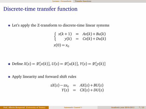
Discrete-time transfer function

Let’s apply the Z-transform to discrete-time linear systems

§

x(k+ 1) = Ax(k) + Bu(k)y(k) = Cx(k) +Du(k)

x(0) = x0

Define X(z) =Z [x(k)], U(z) =Z [u(k)], Y(z) =Z [y(k)]

Apply linearity and forward shift rules

zX(z)− zx0 = AX(z) + BU(z)Y(z) = CX(z) +DU(z)




X(z) = z(zI− A)−1x0 + (zI− A)−1BU(z)Y(z) = zC(zI− A)−1x0

︸︷︷︸

Z-transform

of natural response

+(C(zI− A)−1B+D)U(z)︸︷︷︸

Z-transform

of forced response

Definition:

The transfer function of a discrete-time linear system (A, B, C, D) is the ratio

G(z) = C(zI− A)−1B+D

between the Z-transform Y(z) of the output and the Z-transform U(z) of the inputsignals for the initial state x0 = 0

MATLAB»sys=ss(A,B,C,D,Ts);»G=tf(sys)




A;B;C;D G(z)u(k) y(k) U(z) Y (z)

x0 = 0

Example: The linear system

x(k+ 1) =�

0.5 10 −0.5

�

x(k) +�

01

�

u(k)

y(k) =�

1 −1�

x(k)

with sampling time Ts = 0.1 s has the transfer function

G(z) =−z+ 1.5z2 − 0.25

Note: Even for discrete-time systems, thetransfer function does not depend on the inputu(k). It’s only a property of the linear system

MATLAB»sys=ss([0.5 1;0 -0.5],[0;1],[1 -1],0,0.1);

»G=tf(sys)

Transfer function:-z + 1.5----------sˆ2 - 0.25


Lecture: Z-transform Difference equation

Difference equations

Consider the nth-order difference equation forced by u

any(k− n) + an−1y(k− n+ 1) + · · ·+ a1y(k− 1) + y(k)= bnu(k− n) + · · ·+ b1u(k− 1)

For zero initial conditions we get the transfer function

G(z) =bnz−n + bn−1z−n+1 + · · ·+ b1z−1

anz−n + an−1z−n+1 + · · ·+ a1z−1 + 1

=b1zn−1 + · · ·+ bn−1z+ bn

zn + a1zn−1 + · · ·+ an−1z+ an



Difference equations

Example: 3y(k− 2) + 2y(k− 1) + y(k) = 2u(k− 1)

G(z) =2z−1

3z−2 + 2z−1 + 1=

2zz2 + 2z+ 3

Note: The same transfer function G(z) is obtained from the equivalent matrixform

x(k+ 1) =�

0 1−3 −2

�

x(k) +�

01

�

u(k)

y(k) =�

0 2�

x(k)

⇒ G(z) =�

0 2�

�

z�

1 00 1

�

−�

0 1−3 −2

��−1 � 01

�



Some common transfer functions

Integrator§

x(k+ 1) = x(k) + u(k)y(k) = x(k)

U(z) Y (z)

z ¡ 11

Double integrator

x1(k+ 1) = x1(k) + x2(k)x2(k+ 1) = x2(k) + u(k)

y(k) = x1(k)

U(z) Y (z)

z2¡ 2z + 1

1



Some common transfer functions

Oscillator

x1(k+ 1) = x1(k)− x2(k) + u(k)x2(k+ 1) = x1(k)

y(k) = 12 x1(k) +

12 x2(k)

U(z) Y (z)1

2z + 1

2

z2¡ z + 1

0 10 20 30 40 50 60−2

−1

0

1

2output response

y(k)

k



Impulse response

Consider the impulsive input u(k) = δ(k), U(z) = 1. The correspondingoutput y(k) is called impulse response

The Z-transform of y(k) is Y(z) = G(z) · 1= G(z)Therefore the impulse response coincides with the inverse Z-transform g(k) ofthe transfer function G(z)

Example (integrator:)

u(k) = δ(k)y(k) = Z−1

�

1z−1

�

= 1I(k− 1)−2 0 2 4 6 8 10

−2

−1

0

1

2

u(k

)

k−2 0 2 4 6 8 10

−2

−1

0

1

2

y(k

)

k



Poles, eigenvalues, modes

Linear discrete-time system

§

x(k+ 1) = Ax(k) + Bu(k)y(k) = Cx(k) +Du(k)

x(0) = 0G(z) = C(zI− A)−1B+D¬

NG(z)DG(z)

Use the adjugate matrix to represent the inverse of zI− A

C(zI− A)−1B+D=C Adj(zI− A)B

det(zI− A)+D

The denominator DG(z) = det(zI− A) !

The poles of G(z) coincide with the eigenvalues of A

Well, as in continuous-time, not always ...



Steady-state solution and DC gain

Let A asymptotically stable (|λi|< 1). Natural response vanishesasymptoticallyAssume constant u(k)≡ ur, ∀k ∈ N. What is the asymptotic valuexr = limk→∞x(k) ?

Impose xr(k+ 1) = xr(k) = Axr + Bur and get xr = (I− A)−1Bur

The corresponding steady-state output yr = Cxr +Dur is

yr = (C(I− A)−1B+D)︸︷︷︸

DC gain

ur

Cf. final value theorem:

yr = limk→+∞

y(k) = limz→1(z− 1)Y(z)

= limz→1(z− 1)G(z)U(z) = lim

z→1(z− 1)G(z)

urzz− 1

= G(1)ur = (C(I− A)−1B+D)ur

G(1) is called the DC gain of the systemProf. Alberto Bemporad (University of Trento) Automatic Control 1 Academic year 2010-2011 16 / 21


Example - Student dynamics

Recall student dynamics in 3-years undergraduate course

x(k+ 1) =

.2 0 0

.6 .15 00 .8 .08

x(k) +

100

u(k)

y(k) =�

0 0 .9�

x(k)

DC gain:

[ 0 0 .9 ]�� 1 0 0

0 1 00 0 1

�

−� .2 0 0

.6 .15 00 .8 .08

��−1 � 100

�

≈ 0.69

Transfer function: G(z) = 0.432z3−0.43z2+0.058z−0.0024 , G(1)≈ 0.69

2006 2008 2010 2012 2014 20160

5

10

15

20

25

30

35y(k)

step k

MATLAB»A=[b1 0 0; a1 b2 0; 0 a2 b3];»B=[1;0;0];»C=[0 0 a3];»D=[0];»sys=ss(A,B,C,D,1);»dcgain(sys)

ans =

0.6905

For u(k)≡ 50 students enrolled steadily, y(k)→ 0.69 · 50≈ 34.5 graduateProf. Alberto Bemporad (University of Trento) Automatic Control 1 Academic year 2010-2011 17 / 21

Lecture: Z-transform Algebraically equivalent systems

Linear algebra recalls: Change of coordinates

Let {v1, . . . , vn} be a basis of Rn (= n linearly independent vectors)

The canonical basis of Rn is e1 =

10...0

, e2 =

01...0

, . . ., en =

0...01

A vector w ∈ Rn can be expressed as a linear combination of the basis vectors,whose coefficients are the coordinates in the corresponding basis

w=n∑

i=1

xiei =n∑

i=1

zivi

The relation between the coordinates x = [x1 . . . xn]′ in the canonical basisand the coordinates z= [z1 . . . zn]′ in the new basis is

x = Tz

where T =�

v1 . . . vn

�

(= coordinate transformation matrix)



Algebraically equivalent systems

Consider the linear system�

x(k+ 1) = Ax(k) + Bu(k)

y(k) = Cx(k) +Du(k)

x(0) = x0

Let T be invertible and define the change of coordinates x = Tz, z= T−1x§

z(k+ 1) = T−1x(k+ 1) = T−1 (Ax(k) + Bu(k)) = T−1ATz(k) + T−1Bu(k)y(k) = CTz(k) +Du(k)

z0 = T−1x0

and hence§

z(k+ 1) = Az(k) + Bu(k)y(k) = Cz(k) + Du(k)

z(0) = T−1x0

The dynamical systems (A, B, C, D) and (A, B, C, D) are called algebraicallyequivalent



Transfer function of algebraically equivalent systems

Consider two algebraically equivalent systems (A, B, C, D) and (A, B, C, D)

A= T−1AT C = CTB= T−1B D= D

(A, B, C, D) and (A, B, C, D) have the same transfer functions:

G(z) = C(zI− A)−1B+ D= CT(zT−1IT − T−1AT)−1T−1B+D= CTT−1(zI− A)TT−1B+D= C(zI− A)−1B+D= G(z)

The same result holds for continuous-time linear systems



English-Italian Vocabulary

Z-transform trasformata zetaforward shift operator operatore di anticipounit delay ritardo unitario

Translation is obvious otherwise.


z-transform - imt school for advanced studies...

Documents