Yun, X., Brooks, S., Cheng, Y., Hales, A., Lucas, E., McBryde, D., &Quarini, J. (2015). Ice formation in the subcooled brine environment.International Journal of Heat and Mass Transfer, 95, 198 - 205. DOI:10.1016/j.ijheatmasstransfer.2015.12.003

Peer reviewed version

Link to published version (if available):10.1016/j.ijheatmasstransfer.2015.12.003

Link to publication record in Explore Bristol ResearchPDF-document

University of Bristol - Explore Bristol ResearchGeneral rights

This document is made available in accordance with publisher policies. Please cite only the publishedversion using the reference above. Full terms of use are available:http://www.bristol.ac.uk/pure/about/ebr-terms

Ice formation in the subcooled brine environment

Abstract

Generating ice in a fluid immiscible with water is relatively easy but considerablymore difficult if the chosen fluid is hydrophilic. Our experimental work showed that,ice can be produced when water is introduced to a bath of subcooled brine and it wasbelieved that, the rate of heat transfer between the two fluids needs to be higher thanthat of mass transfer to allow the formation of ice to occur as a result. Flow rheology,hence the size of the active surface area of the injected water stream, brine temperatureand concentration are the key factors influencing how much ice can be made in theprocess. Conversion ratios of two ice collection methods are compared over a rangeof brine temperatures and concentrations. The washing method (wet collection) wasfound to collect up to 27% more ice than dry collection. Washing is also very effectivein rinsing off the brine and salt on the ice’s surface and the bulk salinity would dropfrom 13% to 1%. Since the evaporator temperature has to be higher than the eutecticpoint of brine, it was suggested that, the coefficient of performance, COP, will be verypromising. In addition, this way of ice production should achieve higher efficiency thana scraped surface ice maker and it is simpler in that it requires no complex mechanicalharvesting equipment, and with the vast liquid-liquid surface areas possible, promisesto be able to produce high quantities of ice per unit volume of equipment.

1 Introduction

Ice slurries have a wide range of engineering applications. Due to the latent heat of fusionof ice which results in their high energy storage capacity, ice slurries are used as secondaryrefrigerant for thermal storage systems [1–3]. Another successful application of ice slurries isthe ice pigging technology [4] which is now commercially used in water and food industries.Researches to employ this technology in hydrocarbon industry are also being conducted [5].

It is inherently difficult to achieve a high rate of ice production in industrial environmentswith simple, easy to maintain equipments whilst pursuing high coefficient of performances,COP. Amongst the existing ice slurry generation mechanisms [2,6–14], scraped surface is themost widely utilised. With a type of freezing point depressant (FPD) added in water, icewould nucleate and propagate on a cold metal surface before it can further develop into amushy layer. As the mushy layer thickens on the subcooled surface, it acts as an insulatorwhich reduces the rate of heat transfer and ice formation. For this reason, it is then required

1

to shear off the ice by a mechanical scraper or, less popular, an energy inefficient thermalcycling system to keep the ice layer thin. The mushy layer removal systems require highmaintenance cost and increase the size of the equipments. The undesirable growth of iceon cold evaporator surfaces is also a problem for both industrial and domestic freezers anddeicing has to be performed on a regular basis [15,16].

A cheaper and more efficient way of generating ice slurries has two separate stages. Inthe first stage, water is frozen on a cold surface which is cyclically heated to remove theice once it has reached a certain thickness [17]. Comminution of this bulk ice with brinesupplement then completes the process [18]. Per kilogram of ice slurry, this method canreduce energy usage by 32% compared to a scraped surface ice maker provided that theevaporator temperature is elevated by 20℃, from -30℃ to -10℃ and energy consumptionof any auxiliary systems are disregarded [19]. With the ice storage and delivery taken intoconsideration, 20% of saving maybe achievable in practice [20]. As for the implementationon ice pigging, the pig is produced at the point of delivery where bulk ice is crushed intothe correct size, instead of being generated overnight and stored and maintained in a stirrertank where more power is consumed. Although this way of ice slurry generation is moreefficient, it is easy to have the crushed ice to stick together and become larger pieces if theadded brine does not fill up the gap between ice particles soon enough and consequentlymakes it difficult to carry out the ‘cafetiere test’ [21,22] to detect the ice fraction. Whetherthe quality of the ice slurries would affect electromagnetic wave attenuation which can beused as the fundamental principle of an online ice fraction detection method [23] is not wellunderstood yet. Another method considered inexpensive is to produce ice slurries or flakeice by means of direct contact which requires neither subcooled surfaces nor mechanisms tomaintain the rate of production [10–14]. However, this way of ice production requires themixing of water, refrigerant and compressor oil, making it suitable for the thermal storageapplication but cannot be implemented in the food industry.

In this study, a novel method of ice production is proposed whereby ice is generated ina fluid with a temperature below the freezing point of water. Water at about 0℃ is intro-duced into a bath of brine with a range of salt concentrations by weight (from eutectic point,23.3% to 21%), at temperatures of about -18℃. Provided the rate of transient heat transferexceeds that of mass transfer so that the latent heat of fusion can diffuse away quickly, icewould form. Experimental progress is presented in this paper.

Nomenclature

α thermal diffusivity

∆Gv Gibbs energy per unit volume

∆T bath supercooling temperature

2

∆TSLSH unuseful superheat in the suction line

ηisen isentropic efficiency

ηvol volumetric efficiency

ν growth rate of ice

φ†v cafetiere ice fraction

σ Surface energy

A area

a constant

CB wt% salt in brine

Cw wt% salt in water

D mass diffusivity

Gr Grashof number

Grm mass transfer Grashof number

hh heat transfer coefficient

hm mass transfer coefficient

m mass transfer

Nu Nusselt number

Pr Prandtl number

Q available cooling by the refrigeration cycle

q heat transfer

r∗ Critical radius for nucleation

Ra Rayleigh number

Ram mass transfer Rayleigh number

Re Reynolds number

Sc Schmidt number

Sh Sherwood number

3

TB brine temperature

TC compressor temperature

TE evaporator temperature

Tw water temperature

W ∗ Critical energy for nucleation

Wc compressor work

COP coefficient of performance

2 Background

2.1 Preliminary experimental observations

It is relatively easy to generate ice when the heat sink fluid is immiscible with water, as inthe direct contact method, but considerably more demanding if brine is used instead be-cause water can easily mix with the cooling media in this later case. There are two real lifeexamples that enlightened us to consider making ice with a choice of hydrophilic solutionand both of them are based on the fact that heat transfer can be higher than mass transferin fluids.

The first is the simple water droplet experiment, which is performed by releasing a fewdrops of water to the surface of a bath of cold brine. If the brine temperature is muchlower than 0℃, a disc of ice would form. This phenomenon indicates that the transientheat transfer, mainly by conduction, is higher than mass transfer and the Lewis Number,Le = Sc/Pr = α/D, which measures the relative boundary layer thickness of temperatureand concentration, in this case should be greater than unity.

Another high Le number example is found in a bottle of naturally stratified brine at aconcentration below its saturation. Despite it is well mixed in the first place, a concentra-tion gradient will slowly develop along the bottle and eventually remain unchanged if it isleft untouched long enough in a room where the ambient temperature fluctuates from dayto nigh; at some point, mass transfer will almost stop while heat transfer continues.

These two observations shows that it is possible to produce ice through introducing waterto a bath of subcooled brine provided that the heat and mass transfer is carefully controlledso that the latent heat of fusion can dissipate away from the boundary layer before phasetransformation completes.

4

2.2 Heat and mass transfer fundamentals

Water has low value of thermal conductivity (∼0.5 W/mK) and convection of mass, whichconsists of advection and diffusion, makes it a good heat transfer media. The driving force ofadvection is the temperature and concentration led density difference that initiates buoyancywith the presence of gravity. Heat and mass transfer can be expressed in Equation 1a and1b where hh and hm are heat and mas transfer coefficient governed by a range of physicalproperties.

q = Ahh(Tw − TB) (1a)

m = Ahm(Cw − CB) (1b)

hh can be determined through the Nusselt number, Nu. In most cases, Nu is a func-tion of the Rayleigh number, Ra, and the Prandtl number, Pr, for natural convection only(Gr/Re2 � 1); if not, Nu is a function of Ra alone (2a). In forced convection scenario(Gr/Re2 � 1), Nu is a function of the Reynolds number, Re, and Pr (2b). If neitherconvective regime dominates (Gr/Re2 ≈ 1), Nu is a function of Re, Gr and Pr; natural andforced convections are in the same order of magnitude (2c) [24–27].

In natural convection, the boundary layer flow would remain laminar if the distance ithas travelled is short enough so that the Grashof number, Gr, is below the order of 9 fora wide range of fluids with various Pr values. One can also use Ra ∼ 109, by recallingthat Ra = GrPr, as the critical value that marks the transition of a natural convectivestream. [28]

Nu = f(Ra, (Pr)) (2a)

Nu = f(Re, Pr) (2b)

Nu = f(Re,Gr, Pr) (2c)

In the heat and mass transfer analogy, the counterpart ofNu is the Sherwood number, Sh,which gives hm, and the Schmidt number, Sh, substitutes Pr. By replacing the temperatureterms with concentration, the corresponding mass transfer Rayleigh number, Ram, and masstransfer Grashof number, Grm, are used in mass transfer problems. As in the heat transferanalysis, the Re is only considered in the mixed convection scenario (3c) or will dominatethe mass transfer in forced convection (3b).

Sh = f(Ram, (Sc)) (3a)

Sh = f(Re, Sc) (3b)

Sh = f(Re,Grm, Sc) (3c)

5

2.3 Crystallisation: nucleation and growth

Ice Ih-like hydrogen-bonded clusters are the only molecular groups that can occasionallygrow by statistical fluctuations into a stable size and become nucleation sites [29]. Theminimum energy required for the existing clusters to develop into a size that do not dissolveback to the bulk fluid is

W ∗ =16πσ3

3 (∆Gv)2 (4)

and the corresponding critical radius is

r∗ =2σ

∆Gv

(5)

Once these nucleation sites have bypassed their critical radii, the subsequent rate ofdendritic propagation of ice will be very fast and can be expressed in the form of ν = a(∆T )n

[30–32]. In rapid solidification, the growth of solids can be further subdivided into threeconfigurations: needle invasion, consolidation and plateau [33]. The rapid solidificationalways has an S-shaped history and is in accord with constructal law [34].

3 Apparatus and procedure

3.1 Experimental apparatus

There are two sets of cooling equipments used to carry out the study. The first is the modi-fied Gelato Chef 2200 ice cream maker with a 1.5 litre aluminium container. It is employedto observe effects of water injection position, flow rheology and brine temperature on iceformation. A digital thermometer detects the temperature of the brine in the containerthroughout the experiments. The thermometer is made of a K-type thermocouple. Theexperiment recorded in Video 1 used these equipments.

The experimental apparatus setup illustrated in Figure 1 is later utilised to quantify howmuch ice can be produced for a given mass of water introduced. The tank is filled up byroughly 30 litres of brine at a range of concentrations. The temperature of the fluid ismaintained by a refrigeration unit which uses R134a and its evaporator, at about -30℃, issubmerged in the liquid. To control the brine temperature, an aquarium heater is installedat the base of the tank and it is switched on by a control unit if the brine temperature, mea-sured by a K-type thermocouple, falls below the preset value. In addition, a small aquariumpump (200 litre/hour) is placed in the tank to assist the heat transfer between the coldevaporator and the bulk fluid by generating a flow to eliminate the growth of hydrohaliteand ice on the evaporator’s surface. This pump is only switched on between experimentsand is off before the experiment starts so that the fluid is quiescent; there is no bulk fluidmotion in the brine phase. The experiment recorded in Video 2 used this setup.

6

Water is delivered and injected to the cold brine by a glass syringe (100 ml capacity) with2mm diameter silicone tube attached to its end. The syringe is placed on a table whoseheight can be adjusted, so to alter the siphon hydrostatic pressure between the inlet (exit ofsyringe) and outlet of the tube. The flow rate of the water stream can therefore be controlledin this way. Both Video 1 and 2 adopt these equipments when delivering water to the bulkbrine. The apparatus used to measure the density of the melted ice solution is the AntonPaar DMA 4500 M. Ice slurries are produced from the ZIEGRA ice machine Model SI 1000and the brine salinity by weight is set at 5%.

Suction Line

Liquid Line(Capillary Tube)

EvaporatorRefrigeration

UnitBrine Tank

Injection Syringe

Silicone Tube

Figure 1: Schematic diagram of experimental apparatus

3.2 Experimental procedure

With the Gelato Chef 2200 setup (Video 1), brine at eutectic concentration is preparedand kept at about -20℃ in a freezer and then poured into the 1.5 litre container where thetemperature of the fluid is tracked by the K-type thermometer. The cooling unit is thenswitched on. The cold evaporator surfaces are in contact with the walls of the container tokeep the brine cold. The water to be introduced to the brine is cooled in the same freezer to2℃ and then sucked into the glass syringe. The differences between releasing water dropletsabove brine surface and injecting it through the bulk fluid, from the syringe, is comparedat first (Section 4.1). To ensure the water temperature at the outlet of the tube are thesame for both cases, a fixed length of tube is submerged in the brine and the flow ratesare kept identical by adjusting the position of the syringe through the height of the table.Flow rheology can be managed through adjusting the outlet angles as illustrated in Figure2. The outlet angle can be managed between 90° (Figure 2a) and 0° (Figure 2b) to thehorizontal axis. The water stream in the second case, Figure 2b, only has the horizontalvelocity component which would result the flow having the highest active surface area withthe subcooled liquid (Video 1 and 2). The variation of flow rheology is achieved by adjustingthe outlet angle. The change of the rheology of the flow alters surface area over volume ratioof the water stream and it is discussed in Section 4.2. In the last set of experiments with thislower cooling capacity refrigeration system, qualitative effects of brine temperature on theformation of ice is observed. The observations are included in the first paragraph of Section

7

4.3 of this paper.

(a) (b)

Figure 2: Flow rheology control

To quantify how much water is converted into ice, 100 ml of water, at 2℃ as in before,is introduce in each experiment across a range of brine temperatures. After each injection,the ice is collected by a finely meshed sieve and weighted on an electronic scale. The sieveis shown in Figure 13b and 13c. There are two ice collection regimes used. In the first, iceis scooped out by the sieve and shook only, whereas it is washed, by 0℃ water, as soon asit is taken out of the tank in the other. The comparison of the two collection regimes canbe found in the second paragraph of Section 4.3. Collected ice’s density is measured by thedensity metre once the collected ice is fully melt; the salt concentration by weight in theice is then derived from this value with reference to Lide [35]. To validate the experimentalresults from this handbook, we have done some tests and these values match with what wererecorded in our lab. The handbook also provides the correlation between brine density andsalt concentration by weight. By subtracting the salt mass from the measured value, the netmass of ice collected is obtained; water to ice conversion ratio is hence derived from the netweight of ice.

4 Experimental results and discussion

4.1 Water injection position

The comparison between releasing water droplets above brine surface and injecting it throughthe bulk fluid, at -16℃ , is shown in Figure 3. When water is introduced to the brine surface(Figure 3a), due to its lower density, it will stay on the top of the subcooled environment andnucleate quickly. The subsequent crystal growth is fast and then slows down. The reasonthat leads to the reduction in growth rate is because both water and ice are lighter than thebrine and they will float on the top of the brine surface and conduction is therefore the formof heat transfer. Since water is poor conductor, the latent heat of fusion of ice will quickly

8

heat up the surrounding fluid right adjacent to the freezing frontier and cannot be transportto the bulk fluid through mass transfer in form of advection. The rise in local temperaturehence slows down the rate of phase transformation.

If water is injected through the brine (Figure 3b), the introduced water will nucleate andpropagate on its way to the brine surface and form a rod of ice if the tube exit is kept upright(at 90° to the horizontal axis) as illustrated in Figure 2a. The bulk motion of the streamhas enhanced both heat and mass transfer. Advection makes ice to grow faster whereasencourages water to mix with the brine at the same time. The escaping of the unfrozenwater away from the freezing frontier can be clearly seen in Video 2.

(a) Above brine surface (b) From inside brine

Figure 3: Water injection position comparison

4.2 Flow rheology and area over volume ratio

It was observed that reducing the flow rate does not encourage more ice to be formed buttube blockage. This is because more sensible heat has been extracted when water is still inthe tube and it can easily be supercooled and become ice once nucleation is triggered.

Flow rheology, managed by altering vertical and horizontal velocity component of the flow(Figure 2), however has a significant impact on ice formation. Figure 4 and Video 1 showedthat, a ‘sheet’ of ice was produced if the injected water stream only had the horizontal ve-locity component (Figure 2b). The ‘sheet’ of ice is always reproducible. If, however, theoutlet is kept upright (Figure 2a), a rod of ice may not always appear although the flow rateis kept identical. Pure mixing often happens when water is injected by this way.

The major difference, except the initial vertical velocity, between the two types of injec-tions is the active surface area and hence the area over volume ratio of the stream. Area ofcontact is a key factor that affects both the rate of heat and mass transfer. According to

9

the Chilton-Colburn analogy, the change in heat and mass transfer should essentially be thesame, however, our experiments have shown otherwise because more ice is generated phasetransformation is much more stable when the active surface area is increased. Ice formationcertainly has direct correlation to the active surface area and area over volume ratio of thestream. The experiments carried out in Section 4.3 and 4.5 use 0° injection angle.

Figure 4: Flow rheology control

4.3 Effects of brine temperature

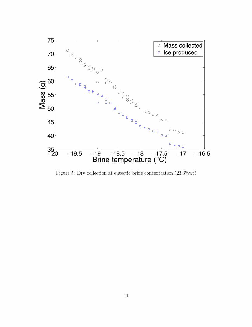
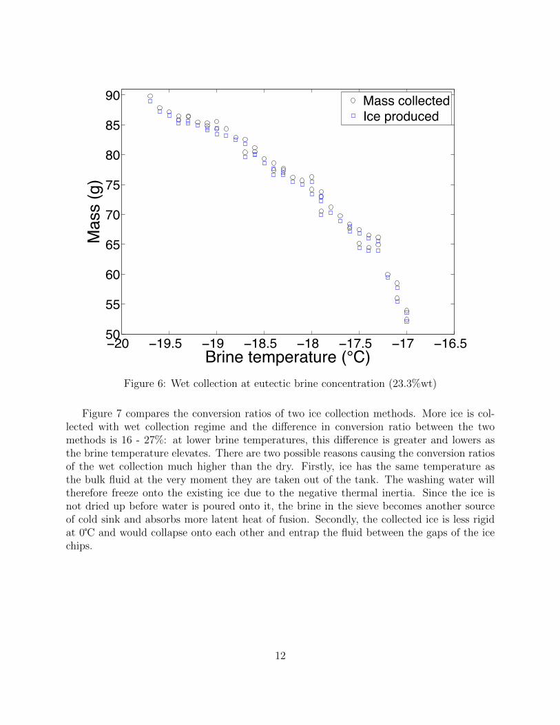
It was found that, brine temperature has a strong impact on water to ice conversion ratio.Figure 5 and 6 illustrated the variation in collected mass and mass of ice produced for dryand wet ice collections. Experimental results become unstable when the bath temperatureis -17℃ or higher and only the temperature range presented in these figures is studied. Ifthe brine temperature is elevated up to about -13℃, ice can hardly produced by means ofinjection through the brine. Brine temperature also affects heat and mass transfer betweenice and the liquid after ice is generated. At higher bath temperature, ice tends to melt faster.

10

−20 −19.5 −19 −18.5 −18 −17.5 −17 −16.535

40

45

50

55

60

65

70

75

Brine temperature (°C)

Mas

s (g

)

Mass collectedIce produced

Figure 5: Dry collection at eutectic brine concentration (23.3%wt)

11

−20 −19.5 −19 −18.5 −18 −17.5 −17 −16.550

55

60

65

70

75

80

85

90

Brine temperature (°C)

Mas

s (g

)

Mass collectedIce produced

Figure 6: Wet collection at eutectic brine concentration (23.3%wt)

Figure 7 compares the conversion ratios of two ice collection methods. More ice is col-lected with wet collection regime and the difference in conversion ratio between the twomethods is 16 - 27%: at lower brine temperatures, this difference is greater and lowers asthe brine temperature elevates. There are two possible reasons causing the conversion ratiosof the wet collection much higher than the dry. Firstly, ice has the same temperature asthe bulk fluid at the very moment they are taken out of the tank. The washing water willtherefore freeze onto the existing ice due to the negative thermal inertia. Since the ice isnot dried up before water is poured onto it, the brine in the sieve becomes another sourceof cold sink and absorbs more latent heat of fusion. Secondly, the collected ice is less rigidat 0℃ and would collapse onto each other and entrap the fluid between the gaps of the icechips.

12

−20 −19.5 −19 −18.5 −18 −17.5 −17 −16.50.3

0.4

0.5

0.6

0.7

0.8

0.9

1

Brine temperature (°C)

Con

vers

ion

ratio

Dry collectionWet collection

Figure 7: Conversion ratio vs. brine temperature at eutectic brine concentration (23.3%wt)

4.4 Salt entrapment

On average, bulk salinity of the dry collected ice is at about 13% and 1% for the washedice (Figure 8). The action of washing the ice is very effective in rinsing off the brine andsalt that stays on the ice surface. The high salt concentration of the ice in dry collectionis quite likely due to the large active surface area, which encourages brine and salt to clingonto the ice. The surface of the generated ice also has rough texture because of the dendriticgrowth that occurs on the boundary layer where the fluid has a certain degree of mixing. Theirregular morphology of these dendrites can trap more rejected salt and high salinity brineonto the ice surface, which effectively elevates the bulk salt concentration of the collectedmaterial. The low bulk salinity of the wet collection regime also indicates that, the amountof salt entrapped within the thin ice’s structure is negligible. In addition, the salinity of thecold bath, which is between 21% and eutectic point, has no effects on the amount of saltcollected with the ice sample at this level of salt concentration.

13

−20 −19.5 −19 −18.5 −18 −17.5 −17 −16.50

5

10

15

Brine temperature (°C)

Salin

ity o

f col

lect

ed ic

e (w

t%)

Dry collectionWet collection

Figure 8: Ice sample salinity vs. brine temperature

The ice particles of ice slurries have low area over volume ratio and this ratio must belower than the very thin ice ‘sheets’ produced by our method. To compare the difference insalt content after washing the two types of ice, ice slurries with bulk salinity of 5% is washedwith 0℃ water and well shook. It was found that, salt concentrations of the washed ice slur-ries have strong correlation to the cafetiere ice fraction and therefore, the salt concentrationof the brine phase and the temperature of the suspension (Figure 9 - 11). However, it is notvery clear if the area over volume ratio of the ice affects the salt content after washing isperformed from these figures. The percentage error of the cafetiere test is 3% [22] and theuncertainty of each salt concentration of the brine phase and the ice slurry temperature arecalculated from the corresponding values of φ†v.

At higher ice fraction, where the temperature of the ice slurry is lower, the 0℃ washingwater tends to freeze and form a thin crust, which barricades the upcoming liquid fromrinsing the ice further. The chance of the generation of such shield is very sensitive with icefraction and the water has more chances to travel through the gaps between the ice particlesand lowers the salt concentration as the ice fraction drops. The 60 - 70% ice fraction rangelooks like the transitional value whence the salinity of the washed ice falls down to a low

14

level similar to that in the wet collection scenario in Section 4.3.

0.3 0.4 0.5 0.6 0.7 0.8 0.90.5

1

1.5

2

2.5

3

Cafetière ice fraction, φv†

Salin

ity o

f was

hed

ice

slur

ries

(wt%

)

Figure 9: Slurry salinity vs. cafetiere ice fraction

15

7 8 9 10 110.5

1

1.5

2

2.5

3Sa

linity

of w

ashe

d ic

e sl

urrie

s(w

t%)

Salinity of brine phase (wt%)

Figure 10: Slurry salinity vs. brine phase salinity

16

−8−7−6−5−40.5

1

1.5

2

2.5

3

Ice slurry temperature (°C)

Salin

ity o

f was

hed

ice

slur

ries

(wt%

)

Figure 11: Slurry salinity vs. temperature

4.5 Effects of brine concentration

The change of the brine concentration alters the ‘driving force’ to mass transfer (Cw−CB) andthe conversion ratios are found improved by reducing the brine concentration from eutecticpoint. Figure 12 compares the conversion ratios of three brine concentrations (23.3%, 22%and 21%) and best fit lines are plotted with the data. The experiments were carried outat a range of bath temperatures. The conversion ratio drops linearly with the elevation ofbrine temperature in the cold bath in the form of f(TB) = p1 × TB + p2 where p1 and p2are coefficients. The values of these coefficients are listed in Table 1 for the studied brineconcentrations.

17

−20 −19.5 −19 −18.5 −18 −17.5 −17 −16.5

0.4

0.5

0.6

0.7

0.8

0.9

1

Brine temperature (°C)

Con

vers

ion

ratio

Dry collection 23.3%wtDry collection 22%wtDry collection 21%wtWet collection 23.3%wtWet collection 22%wtWet collection 21%wtDry collection 23.3%wt best fitDry collection 22%wt best fitDry collection 21%wt best fitWet collection 23.3%wt best fitWet collection 22%wt best fitWet collection 21%wt best fit

Figure 12: Conversion ratio comparison at different brine concentration with best fit line

Table 1: Coefficients of the best fit lines

Dry collection Wet collectionSalt concentration (%wt) p1 p2 p1 p2

23.3% -0.09909 -1.34 -0.1196 -1.43922% -0.1204 -1.633 -0.1439 -1.83921% -0.1261 -1.682 -0.1545 -1.98

4.6 Freezing frontier

It is possible, by managing the flow rate and outlet angle, to have phase transformation totake place at a reasonably consistent distance from the tube outlet (Figure 13a and Video 2)and this steady state of ice generation can only be disturbed if the travelling ice reaches thebrine surface. The location of the freezing frontier has evident impact on the morphologyof the ice produced. Without phase transformation, the flow becomes more turbulent as it

18

travels further up in the cold environment and the generated ice, provided the ice can form,appears slushier than cases which water turns into ice while the flow is still at its laminarregime (Video 2). The morphology of ice generated in laminar and turbulent region arecompared in Figure 13b and 13c.

19

(a) Freezing frontier

(b) Sample ice formed in laminar region

(c) Sample ice formed in turbulent region

Figure 13: Freezing frontier and collected ice sample

20

5 Optimisation of the cooling system

5.1 Evaporator temperature on COP

The craped surface ice makers require evaporator temperature, TE, to operate at the rangeof -30 to -40℃ to achieve high rate of ice production. With low evaporator temperature,the surface area of the evaporator can be much smaller and hence reduce the size of andweight of the ice machine. The size of the ice maker is important for ice pigging because theequipments need to be shipped to the site of delivery. A low TE, however, has unfavourableeffect to the COP of the refrigeration system since more compressor work is required fora given duty. The COPs invariably worsen significantly as TE drops, as shown in Figure14. The blends, R404a and R57a that are refrigerants made of a number of refrigerants,exhibit slight lower COPs than the already banned and transitional refrigerants, but it is lessignificant compared to the change in TE.

The assumptions made to calculate COPs of a cycle are:

• the compressor is in a healthy state, well lubricated and retains a constant isentropicefficiency, ηisen, of 70%

• pressure losses in suction and discharge line cause the temperature of the fluid to varyby 0.5 K

• useful subcooling and superheating are assumed to be 2 K

• condenser temperature, TC , is assumed constant at 27℃

• unuseful superheat in the suction line, ∆TSLSH , is 2 K

COP is defined by the ratio of available cooling by the refrigeration cycle, Q, and com-pressor work, Wc:

COP =Q

Wc

(6)

Q and Wc are determined by the relevant values of specific enthalpies for each tempera-ture of the studied refrigerants.

In the experiments, the evaporator operates at -30℃ (Section 3.1) which is not much higherthan most scraped surface ice makers, and this low temperature causes hydrohalite and iceto grow on the cold surface; the additional mass transfer generated by the pump is not suf-ficiently strong enough to stop phase transformation on the surface. Since the brine needsto be kept at a relatively quiescent state in order to reduce the chance of turbulence in theinjected water stream, it is impractical to increase the power of the pump but to elevatethe evaporator temperature to somewhere close to the eutectic point of brine and use someextended area of contact to achieve heat transfer needs.

21

Evaporator temperature, TE (°C)-40 -35 -30 -25 -20Co

effic

ient

of p

erfo

rman

ce (C

OP)

1.5

2

2.5

3R502R22R134AR404AR507A

Figure 14: Coefficient of performance over a range of evaporator temperature

5.2 Evaporator and suctionline modification

The assumed 2 K unuseful superheat in the suctionline, as illustrated in Figure 15, causesthe COPs to drop by roughly 1%. The model also suggests that for each 1 K of additionalsuperheat in the suctionline, there is roughly a 0.5% decrease in COP. The amount of heatingress into the refrigerant from the suctionline depends on the design of the system, insu-lation and ambient environment.

Water needs to be cooled down to a temperature close enough to its freezing point. Sincethe refrigerant is still very cold in the suction outlet, it is therefore possible to cascade asecondary heat exchanger between the evaporator outlet and suction inlet to extract thesensible heat from water instead of building another cooling system. In Figure 16, the modelshows that COPs can be further increased by another 5 to 9% provided that the condenserinlet temperature is elevated to 10℃ by the additional cooling duty. In addition, the reduc-tion of pressure ratio between suction and discharge absolute favours volumetric efficiency,ηvol, and hence the compressor efficiency.

22

−40 −35 −30 −25 −201.5

2

2.5

3

Evaporator temperature, TE (°C)

Coe

ffici

ent o

f per

form

ance

(CO

P)

R404A (2 K)R404A (0 K)R507A (2 K)R507A (0 K)

Figure 15: Effects of heat ingress into the suctionline (2 K and 0 K superheat)

23

−40 −35 −30 −25 −201.5

2

2.5

3

Evaporator temperature, TE (°C)

Coe

ffici

ent o

f per

form

ance

(CO

P)

R404AR404AR507AR507A

Figure 16: Effects of modified evaporator and suctionline

6 Conclusions

In practice, the concept of ice generation through introducing water into cold brine methodworks. The buoyancy force discourages mass transfer and therefore mixing if water is in-jected above the brine surface. Rate of growth reduces, as the ice grows thicker due to itslow thermal conductivity. For the case that water is injected in the brine, flow rheology andarea over volume ratio are important factors influencing ice growth. Flow with low level ofturbulence and higher area over volume ratio assists ice generation.

The water to ice conversion ratio is sensitive to brine temperature and it is almost impossi-ble to generate ice when brine temperature is -13℃ or higher. The conversion ratio changeslinearly with the brine temperature. By washing the collected ice, the amount of salt in theice drops from 13% to 1% and the mass of the ice collected would rise by 16 - 27% in thestudied temperature range in comparison with the dry collection method. It was believedthat the combination of the negative thermal inertia of the ice and water entrapment due toice collapsing onto each other are the major reasons causing the difference in conversion ratio.

24

Reducing brine concentration in the cold bath can improve the water to ice conversion ratiounder the studied salinity range. It is preferred to freeze water in its laminar region before ithas turned turbulent because otherwise the level of mixing would rise and ice may not form.The position of freezing frontier has significant effects on morphology of the generated ice.Slushier ice is produced if the injected stream travels further up in the brine.

This way of ice production permits much higher evaporator temperature than the scrapedsurface method which means better COPs of the refrigeration system.

References

[1] C. Chaichana, W. W. Charters, and L. Aye, “An ice thermal storage computer model,”Applied Thermal Engineering, vol. 21, no. 17, pp. 1769 – 1778, 2001.

[2] K. Matsumoto, M. Okada, T. Kawagoe, and C. Kang, “Ice storage system with water–oilmixture: formation of suspension with high {IPF},” International Journal of Refriger-ation, vol. 23, no. 5, pp. 336 – 344, 2000.

[3] M. J. Wang and N. Kusumoto, “Ice slurry based thermal storage in multifunctionalbuildings,” Heat and Mass Transfer, vol. 37, no. 6, pp. 597–604, 2001.

[4] J. Quarini, “Ice-pigging to reduce and remove fouling and to achieve clean-in-place,”Applied Thermal Engineering, vol. 22, no. 7, pp. 747 – 753, 2002.

[5] A. J. Hales, G. Quarini, D. Ash, E. Lucas, and D. McBryde, “The use of ice piggingtechnology to clean shell and tube exchangers,” 13th UK Heat Transfer Conference,UKHTC2013, 2013.

[6] M. B. Lakhdar, R. Cerecero, G. Alvarez, J. Guilpart, D. Flick, and A. Lallemand,“Heat transfer with freezing in a scraped surface heat exchanger,” Applied ThermalEngineering, vol. 25, no. 1, pp. 45 – 60, 2005.

[7] F. G. F. Qin, X. D. Chen, and A. B. Russell, “Heat transfer at the subcooled-scrapedsurface with/without phase change,” AIChE Journal, vol. 49, no. 8, pp. 1947–1955,2003.

[8] J.-P. Bedecarrats, T. David, and J. Castaing-Lasvignottes, “Ice slurry production us-ing supercooling phenomenon,” International Journal of Refrigeration, vol. 33, no. 1,pp. 196 – 204, 2010.

[9] B. Kim, H. Shin, Y. Lee, and J. Jurng, “Study on ice slurry production by water spray,”International Journal of Refrigeration, vol. 24, no. 2, pp. 176 – 184, 2001.

25

[10] M. Hawlader and M. Wahed, “Analyses of ice slurry formation using direct contact heattransfer,” Applied Energy, vol. 86, no. 7–8, pp. 1170 – 1178, 2009.

[11] N. Wijeysundera, M. Hawlader, C. W. B. Andy, and M. Hossain, “Ice-slurry productionusing direct contact heat transfer,” International Journal of Refrigeration, vol. 27, no. 5,pp. 511 – 519, 2004.

[12] T. Kiatsiriroat, K. N. Thalang, and S. Dabbhasuta, “Ice formation around a jet streamof refrigerant,” Energy Conversion and Management, vol. 41, no. 3, pp. 213 – 221, 2000.

[13] T. Kiatsiriroat, S. Vithayasai, N. Vorayos, A. Nuntaphan, and N. Vorayos, “Heat trans-fer prediction for a direct contact ice thermal energy storage,” Energy Conversion andManagement, vol. 44, no. 4, pp. 497 – 508, 2003.

[14] S. Thongwik, N. Vorayos, T. Kiatsiriroat, and A. Nuntaphan, “Thermal analysis ofslurry ice production system using direct contact heat transfer of carbon dioxide andwater mixture,” International Communications in Heat and Mass Transfer, vol. 35,no. 6, pp. 756 – 761, 2008.

[15] A. Bejan, J. V. Vargas, and J. S. Lim, “When to defrost a refrigerator, and when toremove the scale from the heat exchanger of a power plant,” International Journal ofHeat and Mass Transfer, vol. 37, no. 3, pp. 523 – 532, 1994.

[16] V. Radcenco, J. V. C. Vargas, A. Bejan, and J. S. Lim, “Two design aspects of defrostingrefrigerators,” International Journal of Refrigeration, vol. 18, pp. 76 – 86, 2 1995.

[17] J. Vargas and A. Bejan, “Fundamentals of ice making by convection cooling followedby contact melting,” International Journal of Heat and Mass Transfer, vol. 38, no. 15,pp. 2833 – 2841, 1995.

[18] A. Leiper, D. Ash, D. McBryde, and G. Quarini, “Improving the thermal efficiencyof ice slurry production through comminution,” International Journal of Refrigeration,vol. 35, no. 7, pp. 1931 – 1939, 2012.

[19] A. Leiper, Carnot cycle optimisation of ice slurry production through comminution ofbulk ice. Phd thesis, Department of Mechanical Engineering, University of Bristol, 2012.

[20] A. Leiper, E. Hammond, D. Ash, D. McBryde, and G. Quarini, “Energy conservationin ice slurry applications,” Applied Thermal Engineering, vol. 51, no. 1–2, pp. 1255 –1262, 2013.

[21] G. S. F. Shire, The behaviour of ice pigging slurries. Phd thesis, Department of Me-chanical Engineering, University of Bristol, 2006.

[22] T. S. Evans, Technical Aspects of Pipeline Pigging with Flowing Ice Slurries. Phd thesis,Department of Mechanical Engineering, University of Bristol, 2007.

26

[23] A. Hales, G. Quarini, G. Hilton, D. Ash, E. Lucas, D. McBryde, and X. Yun, “Icefraction measurement of ice slurries through electromagnetic attenuation,” InternationalJournal of Refrigeration, vol. 47, pp. 98 – 104, 2014.

[24] H. J. Merk and J. A. Prins, “Thermal convection in laminary boundary layers. i,”Applied Scientific Research, Section A, vol. 4, no. 1, pp. 11–24, 1953.

[25] H. J. Merk and J. A. Prins, “Thermal convection in laminar boundary layers ii,” AppliedScientific Research, Section A, vol. 4, no. 3, pp. 195–206, 1954.

[26] H. J. Merk and J. A. Prins, “Thermal convection in laminar boundary layers iii,” AppliedScientific Research, Section A, vol. 4, no. 3, pp. 207–221, 1954.

[27] J. H. Lienhard(IV) and J. H. Lienhard(V), A Heat Transfer Textbook. PHILOGISTONPRESS, 2008.

[28] A. Bejan, Convection Heat Transfer, 4th Edition. WILEY, 2013.

[29] N. H. Fletcher, The Chemical Physics of Ice. Cambridge U.P., 1970.

[30] C. S. Lindenmeyer and B. Chalmers, “Growth rate of ice dendrites in aqueous solutions,”The Journal of Chemical Physics, vol. 45, no. 8, pp. 2807–2808, 1966.

[31] C. S. Lindenmeyer, G. T. Orrok1, K. A. Jackson, and B. Chalmers, “Rate of growthof ice crystals in supercooled water,” The Journal of Chemical Physics, vol. 27, no. 3,pp. 822–822, 1957.

[32] H. R. Pruppacher, “Some relations between the structure of the ice-solution interfaceand the free growth rate of ice crystals in supercooled aqueous solutions,” Journal ofColloid and Interface Science, vol. 25, no. 2, pp. 285–294, 1967.

[33] A. Bejan, S. Lorente, B. S. Yilbas, and A. Z. Sahin, “Why solidification has an s-shapedhistory,” Scientific Reports, vol. 3, pp. 1711 EP –, 04 2013.

[34] A. Bejan and S. Lorente, “Constructal theory of generation of configuration in natureand engineering,” Journal of Applied Physics, vol. 100, no. 4, 2006.

[35] D. R. Lide, CRC Handbook of Chemistry and Physics. Boca Raton: CRC Press, 86 ed.,2005.

27