yun, geun young and tuohy, p.g. and steemers, k. (2009

1

Title:

Thermal performance of a naturally ventilated building using a combined algorithm of probabilistic

occupant behaviour and deterministic heat and mass balance models

Authors:

Geun Young Yuna, Paul Tuohyb, Koen Steemersa

Affiliation:

a The Martin Centre for Architectural and Urban studies, Department of Architecture, University of

Cambridge, 1-5 Scroope Terrace, Cambridge, UK.

bThe Energy Systems Research Unit, Department of Mechanical Engineering, University of Strathclyde,

Glasgow, UK.

Abstract:

Natural ventilation is an established passive cooling technique with the potential to reduce building energy

demands through the avoidance of air conditioning. However there has been uncertainty about the potential

of natural ventilation in practice due to a lack of knowledge about the occupant interactions with windows

for any given situation. This study explores the role of occupant behaviour in relation to natural ventilation

and its effects on the summer thermal performance of naturally ventilated buildings. A behavioural

algorithm is developed (the Yun algorithm) representing probabilistic occupant behaviour and implemented

within a dynamic simulation tool. A core of this algorithm is the use of Markov chain and Monte Carlo

2

methods in order to integrate probabilistic window use models into dynamic energy simulation procedures.

The comparison between predicted and monitored window use patterns shows good agreement.

Performance of the Yun algorithm is demonstrated for active, medium and passive window users and a

range of office constructions. Results show for example, that in some cases, the temperature of an office

occupied by the active window user in summer is up to 2.6C lower than that for the passive window user.

A comparison is made with results from an alternative behavioural algorithm developed by Humphreys

(Rijal et al., 2007). In general, the two algorithms lead to similar predicted results, but the results suggest

that the Yun algorithm better reflects the observed time of day effects on window use (i.e. the increased

probability of action being taken on arrival).

Keywords:

Natural ventilation, Occupant behaviour, Behavioural algorithm, Window use, Energy efficiency, Thermal

performance, ESP-r, Dynamic building simulation

Corresponding author:

Geun Young Yun

The Martin Centre for Architectural and Urban Studies, Department of Architecture, University of


Phone:+44 (0)1223 760127; Fax: +44 (0)1223 332960 Email: [email protected]

Co-authors:

Paul Tuohy

3

Energy Systems Research Unit, Department of Mechanical Engineering, University of Strathclyde,

Glasgow, UK.

Phone:+44 (0)141 548 3747; Fax: +44 (0)141 552 5105 Email: [email protected]

Koen Steemers

The Martin Centre for Architectural and Urban studies, Department of Architecture, University of


Phone:+44 (0)1223 760127; Fax: +44 (0)1223 332960 Email: [email protected]

1. Introduction

Naturally ventilated buildings are common across many regions of the world. There is an increasing interest

in the comfort and energy performance of these buildings due to a range of factors including higher recent

summer temperatures and also legislative requirements for building energy use and carbon emissions such

as enshrined in the EU directive [1]. One area of concern is the increasing use of air conditioning in UK

buildings and its associated energy and emissions. Avoidance of air conditioning will require buildings to

be designed, built (or re-designed and upgraded) and operated to passively maintain a comfortable indoor

environment. In current UK building regulations, domestic dwellings require a summer overheating

calculation to be carried out using the Governments standard assessment procedure [2] or similar, for non

domestic dwellings the guidance is to use CIBSE TM37 [3]. These methods for demonstrating compliance

are simplistic, set static thresholds and take no explicit account of outside daily or hourly temperature

variations or of detailed building ventilation paths and their dynamic interaction with the external climate.

Other allowed methods include dynamic simulation which can account for dynamic climatic variation.

Although dynamic simulation has the potential to investigate building performance in great detail and

include airflows, ventilation openings, climate and building and occupant detailed behaviour, it is common

4

practice to represent occupant behaviour either by using fixed ventilation rates as in the more simple

methods [2,4] or to model using an indoor temperature threshold to trigger window opening and apply

proportional control above that threshold. The ventilation rates or temperature thresholds are generally

derived from an amalgamation of historical survey data from buildings of a given type to define “typical”

values which could be viewed as representing some typical or average behaviour of occupants. While these

values may well represent behaviour in a historical notional average building they have no ability to

accurately represent or explain the range of behaviours seen in survey data and do not provide insight into

the actual behaviour and resultant effects on energy and comfort that will prevail in a specific situation.

This is especially a concern in the current and future contexts where building regulations, building design,

work patterns and climate are changing and historical assumptions may not be valid.

In a typical naturally ventilated building the performance is highly dependent how the building responds to

climatic and internal variations and on how and when the occupants respond to their conditions (i.e. what

adaptive actions they take and under what conditions will they take them) and in turn how the people’s

adaptive actions alter the buildings performance and so on. In order to model in detail the performance of

naturally ventilated buildings it is desirable to be able to model the occupant’s behaviour within a dynamic

simulation environment. ESP-r is open-source dynamic simulation software developed by ESRU at the

University of Strathclyde [5]. Its open-source nature makes ESP-r a particularly suitable vehicle for the

development and dissemination of new algorithms for adoption in other commercial and non-commercial

simulation tools. Many control modes are already implemented in ESP-r, most represent controls as would

be executed by a building management system (i.e. proportional control, integral control, on/off control and

optimum start control). Some controls have also been implemented to represent occupant behaviour. The

Hunt model [6] for the switching on and off of office lighting, the stochastic Lightswitch 2002 algorithm

developed by Reinhart to predict dynamic personal response and control of lights and blinds from field

study data [7] and Newsham et al [8]’s original Lightswitch model are available. The SHOCC module

developed by Bourgeois et al [9] is also available which enables sub-hourly occupancy modelling coupled

with the occupant behavioural algorithms.

5

Among the most common adaptive actions in a naturally ventilated building is the adjustment of the

window position. Recently the Humphreys adaptive algorithm for window opening behaviour was

implemented in ESP-r and its application illustrated in summer overheating and annual energy use

calculations for a range of different office designs [10, 11]. The Humphreys algorithm is a stochastic

algorithm based on adaptive thermal comfort theory which has evolved over a number of years [12, 13].

The survey data behind the Humphreys algorithm was gathered in the 1990s for a number of offices across

the UK for which window opening was recorded four times per day.

There have been several other studies of window opening behaviour [14, 15, 16, 17, 18] and several

different approaches have been taken in the formulation of algorithms to represent this behaviour. Of

particular interest is the study by Fritsch et al [15]. They performed field measurements of occupants’ use

of windows in four offices during a heating season and proposed Markov chains to create a time series of

window angle as a function of outdoor temperature. The comparison of the monitored and generated time

series of window angles confirmed the validity and reliability of the model based on Markov chains.

Yun and Steemers [19,21] recently carried out a detailed monitoring study at sub-hourly frequency

gathering window use and other environmental data for a number of modern UK offices and developed

occupant window use models based on Markov chains which includes time of day (or more specifically -

time of arrival) as a factor. These models are designed to be applied in Monte Carlo method in order to

capture the non deterministic nature of the window opening behaviour. Time of day effects (i.e. increased

probability of action on arrival etc) on window opening have been recognised by another study [18] and are

also found in other non window behavioural models such as the manual lighting algorithms by Hunt [6] and

Reinhart [7] but are not included in the Humphreys algorithm, possibly due to the time resolution of the

survey data.

6

In this paper a new algorithm (the Yun algorithm) for occupant window-control behaviour in a cellular

office with single-sided natural ventilation and its implementation in dynamic building simulation software

for potential application to building design is described. Predicted behaviour is compared with the

monitored data. The algorithm is then used to demonstrate the effects of a range in user behaviour and

various building design parameters on thermal performance in summer. A comparison is made between the

results from the Yun algorithm and those generated from use of the alternative Humphreys algorithm. The

results, similarities and differences between two approaches are then discussed and some conclusions are

developed.

2. Non-homogenous Markovian model of window states

Yun and Steemers [19] revealed that the previous state of a window strongly influences the current window

state, i.e. the current window state is more likely to stay the same as the previous one, irrespective of the

previous window state. This study has selected a Markov chain model for the representation of occupant

use of a window as a Markovian model is the chance process where the past results have an influence on

the outcomes of successive predictions. The Markovian model has been applied to the simulation of

building performance [22,23,24] and the representation of occupant behaviour [25,26] and occupancy [27].

Tanimoto et al [26], in particular, proposed a method to predict the maximum residential cooling load based

on Markovian models of air-conditioning use and a new algorithm generating the daily activity schedules

of residents. A brief description of the Markov chain is now explained.

2.1 Markov chain

A Markov chain is a sequence of random states, },...,{ ,1,0 rSSSS which meets the following

conditions:

7

)|Pr(),...,,|Pr( 1011 ttttt SSSSSS ( 1)

This definition represents that the distribution of 1tS given the past depends only on the value of the

previous state tS [28]. This Markovian property does not indicate that 1tS is independent of the previous

states, 110 ,..., tSSS , but it means that any dependency of 1tS on the past is stored in the value of

tS [29].

The Markovian process begins in one of the states, S, and proceeds from one state to another in one step.

The transition probability that the chain moves from state i to state j is defined as follows:

)|Pr( 1, iSjSP ttji (2)

The event that a state remains the same occurs with probability of iiP , . If a Markov chain consists of

r states, the equation to calculate the transition probability shifted from state i to state j in m steps is

given by:

r

k

mjkki

mji PPP

1

1,,, (3)

8

2.2 Representing a time series of window states

A time series of the binary state of a window (i.e. open or closed) at time intervals of one-hour has been

constructed using a Markov chain. For the sake of convenience, 0 stands for a window being closed and 1

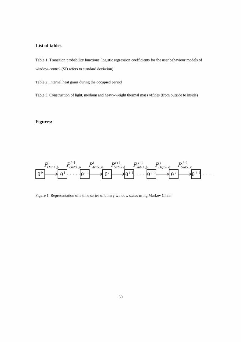
for a window being open. Figure 1 illustrates the sequence of a window state. iP , represents the transition

probability of a window state in i time step from to , where the window state in i time step m is

or . As only two window states are considered here, a window state in m time step

is }1,0{, S . The transition probability is calculated by using the existing occupant behaviour

models of window-control derived from logistic regression analysis [19, 21]. Table 1 summarises occupant

behaviour models as a function of time of day and types of occupants. This Markovian model is

inhomogeneous as the transition probability changes according to the time of day. For instance, the

transition probability of a window state from closed to open on arrival is much higher than the likelihood of

the change of a window state during the subsequent occupation period under the same thermal stimulus.

The subsequent occupation period is defined here as the occupied hours except arrival and departure times.

Insert Figure 1 and Table 1

3. Combined algorithm of probabilistic and deterministic building performance

This study develops an algorithm for probabilistic occupant behaviour integrated with deterministic

building physics models. It aims to comprehend the probabilistic characteristic of the Markovian model of a

window state in the analysis of building performance. The behavioural algorithm borrows the concepts of

stochastic simulations or Monte Carlo methods. A brief explanation of the Monte Carlo methods is now

given.

9

3.1 Monte Carlo method

The Monte Carlo method is defined as a statistical analysis based on artificially recreating chance process

with random numbers, repeating the chance process many times and directly estimating the values of

important parameters [29]. Thus, it provides not just point estimates of interest, but the statistical

characteristic of estimates like average, maximum, minimum, standard deviation, etc. The Monte Carlo

method is based on the law of large numbers, expressed in Equation (4):

Take nXXX ,..., 21 to be independent random variables, with a finite mean ( ). Let

nn XXXS 21 . For every positive real number

0lim

nSP n

n (4)

It indicates that the average of the individual outcomes of random process, (Sn/N), is unlikely to be far

from the true mean ( ), when n is large enough. Therefore, we can obtain the outcome which can be

predicted with a high degree of certainty, by taking averages of independent random processes [30].

3.2 Combined behaviour algorithm of probabilistic occupant behaviour and deterministic heat and

mass balance models

Figure 2 illustrates a combined algorithm of probabilistic and deterministic algorithm of building

performance, developed and subsequently implemented into a building simulation tool, ESP-r. ESP-r is an

integrated modelling tool that simulates a thermal and fluid flow phenomenon in a building, by solving the

thermal model and a fluid flow network. Previous validation studies have shown that ESP-r can accurately

predict thermal and airflow behaviour [31].

10

The first stage in the estimations of indoor thermal conditions and energy demands is to initialise a window

state at a time step of 1 (Figure 2). An initial window state might be randomly chosen from }1,0{S in

the general case. However, the longitudinal field studies [19,21], which provided the transition probability

functions, showed all the windows were closed as occupants left their offices. Thus it is assumed that a

window is closed at the start of a simulation. The algorithm stages from 2 to 5 are carried out at a

simulation time step of i . The second stage assigns a candidate state of a window at the current time step

( i ), which is different from the previous time step ( 1i ). If there are more than two window states, the

candidate state has to be chosen randomly. In this specific case, the candidate state can be simply calculated

by:

|1| (5)

Where is a candidate state at the current time step of i ,

is a window state at the time step of 1i .

Stages 3 and 4 update a window state ( i ) with probability ( iP , ). In other words, they generate a binary

distribution of window states from the transition probability functions in Table 1. In stage 3, the transition

probability of a window state from to is calculated. If the previous window state is closed (=0), then

the equation for the transition probability of a window state to open (=1) at the current time step is given

by

11

1,11

1,01,01

0,01,0 PPPPP iii (6)

Stage 4 is a typical process in Monte Carlo methods [32]. A uniform random variable between 0 and 1 is

created using the pseudo random generator. This random number is compared with the transition

probability calculated in Stage 3. If the transition probability is equal or over the random number, we

accept the trial state (i.e. a window state for the current time step is changed to the trial state). This

evaluation result is then reflected in a time series of a Markovian window states.

Once the window state at the current time step is determined, the iterative solution process of the existing

deterministic thermal and airflow model in ESP-r is started [31]. When the model has converged in Stage 5,

we can attain the point estimate of indoor conditions such as air and mean radiant temperatures, relative

humidity and energy demand. To obtain a window state and other parameters of interest at the next time

step (i+1), repeat the Stages 2 to 5. This is repeated until it reaches the last simulation time step (Stage 6).

Stage 7 is an iteration process (i.e. multiple simulations as a function of a binary distribution of the window

state). It aims to attain the statistical distribution of parameters of interest. Stage 6 is repeated until it meets

the last number of the Monte Carlo or predefined iteration. Each simulation during the iteration process

produces point estimates of indoor thermal conditions and energy demand at each simulation time step. The

final estimates of parameters of interests at each time step in the simulation using the combined algorithm

is the result of the average of point estimates obtained from each of the iterations. Other useful estimates

from the combined algorithm include standard deviation, maximum and minimum values of interest.

Insert Figure 2 here

12

4. Model description

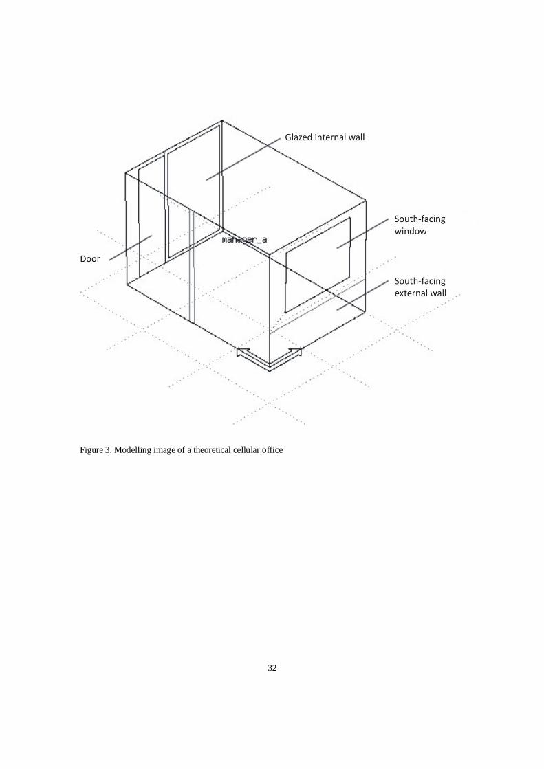
Simulation studies were conducted on a theoretical south facing cellular office (Figure 3). It is assumed that

the office is located within an office building and the thermal conditions of the adjacent space are specified

to be similar to those of the modelled office. The simulations use the climate data set for Cambridge, UK,

obtained from the weather database program, Meteonorm 5.1 [33]. Meteonorm creates hourly weather data

from monthly average values for periods of at least ten years using stochastic methods [33]. The simple

theoretical office model and the climate dataset used in the simulations were chosen to be somewhat similar

to the office types and climate of the monitoring study. Precise details of the monitored buildings such as

thermal and optical properties of constructions, internal gains from equipment and the actual local climate

(including sheltering, ground reflectance and overshading etc.) were not available [19, 21] and so values

have been assumed here to allow the algorithm operation to be demonstrated.

The simple office model whose only external wall faces due south has a width of 3m, a depth of 4.5m and

ceiling height of 3m. The glazing ratio to the total south-facing external wall area is 35% or 3.2m2 and

double glazing with a U-value of 2.8W/m2K was selected. The casual gains in the model are detailed in

Table 2. The modelling study employs different construction types to allow analysis of the effect of thermal

mass. Table 3 shows the specification of each construction type. The simulation period selected to represent

a warm summer period from the Meteonorm climate file is from 21 August (Monday) to 25 August

(Friday). This warm summer period was chosen to represent the type of climatic conditions where a poor

building performance could potentially lead to the adoption of air-conditioning. The simulation time step

used is one hour and the occupied period is from 9 am to 6 pm. The hourly time-step was chosen as being

consistent with the frequency in the monitoring data [19,21].

13

The design light level is 400 lux on a horizontal work plane 0.8m above the floor. For the calculation of

illuminance level on the work plane by daylighting an analytical daylight factor method is selected. The

model has two photocells in the back and front of the space and the average of two photocells illuminance

is used for lighting control to complement the level of daylighting illuminance (Figure 4). An artificial light

is switched off when the daylight level at the height of the work plane is over 600lux (i.e. 1.5 times higher

than design light level).

Two kinds of airflow modelling methods were used. First, an airflow network model, consisting of airflow

components of a large opening, infiltration and external wind pressure, was set up. It was employed for the

simulation of the passive, medium and active behaviour models of window-control. As a comparison the

use of fixed airflows was also evaluated, in this case a fixed constant background infiltration of 0.33 air

change rate per hour (ac/h) was assumed and fixed ventilation rates of 2, 4, or 6ac/h were set during

occupancy, these values were chosen to be within the range specified by CIBSE [4].

Initially the model of the south-facing office with a medium-thermal mass and occupied by the medium

occupant type for window-control was chosen as a base case to allow effective comparison and to highlight

the effects of the various parameters.

Insert Figures 3 and 4 and Tables 2 and 3

5. Results

5.1 Effects of the number of iterations

14

The estimates of indoor conditions are obtained from the average of point estimate results from multiple

simulations (i.e. iterations) as a function of the binary distribution of the window state. Thus, the number of

iterations is of significant importance. To determine the number of iterations required for a stable and

accurate estimation, we investigated the change in indoor operative temperature from the value at the

immediately preceding repetition (Figure 5).

It is observed that variance in the change of the indoor temperature tends to go up as the day goes on. For

instance, the maximum variance is 0.10C at 10 am, 0.38C at 12 pm, 0.68C at 2 pm and 1.00C at 4 pm.

It seems to be attributed to the cumulative effects of probabilistic functions of the window-control

behaviour models at a higher simulation time step. As the time series of window states is represented by

Markov chains, the range of outcomes becomes wider the later the particular simulation step occurs within

the simulation period.

Figure 5 illustrates that only a marginal change in the indoor temperature occurs after 80 iteration

simulations (i.e. 80 numbers of multiple simulations as a function of binary distribution of the window

state). This is in line with previous studies which used Monte Carlo analysis in the uncertainty analysis in

building simulations [33,35]. After 160 iterations the changes in indoor temperature are in most cases less

than 0.01C and the largest change is equal or less than 0.03C. This study has chosen the iterations of 300

to improve and guarantee the accuracy of the simulation results.


5.2 Comparison with monitoring data

15

Due to the lack of some detailed data such as actual local weather conditions, precise thermal properties of

the actual building constructions, and accurate internal heat gains from IT equipment in the field studies

[19,21], a direct comparison of indoor thermal conditions between simulation results and monitoring data

was not possible. Instead, we evaluated the Yun algorithm by comparing the predicted window state to the

measured window state across a range of indoor temperatures. The window state data from simulation

results and the field studies were classified using a temperature bin of 1 ̊C and the probabilities of a window

being open were then calculated according to time of day (i.e. on arrival and during subsequent occupation

period).

The comparison of predicted probabilities using the Yun algorithm with the field monitoring results shows

good agreement (Figure 6), and the monitored and predicted window state probabilities show similar

trends. The difference between the predicted and monitored probabilities is 3.1% for the subsequent

occupation period, which includes all of the occupied period except occupant’s first arrival times. The Yun

algorithm appears to slightly overestimate the probability of a window being open on arrival (the mean

deviation on arrival is 8.6%). However, the difference is not significant considering the unknowns between

the model and the real office.

Insert Figure 6 around here

5.3 The effects of occupant behaviour of window-control

Figure 7a shows the effects of the modelled occupant window opening behaviour on indoor thermal

conditions for a medium window user and also for the case where the window is not opened. The reduction

in the indoor temperature due to window opening behaviour compared to the case where the window is

always closed spans from 1.66C to 9.00C, with an average reduction of 6.18C. The cooling effects of

opening a window become more apparent towards the end of the week due to the cumulative effect of the

16

closed window, ambient temperature and solar and internal gains (figure 7b). For instance, the maximum

temperature difference between when a window is controlled with a medium occupant model of window-

control and when a window is assumed to be closed, takes place on Friday when the peak solar radiation

reaches 669 W/m2. While this model is somewhat simplistic (e.g. it assumes all adjacent spaces in the

building have similar temperatures) it clearly illustrates window opening behaviour as a possible method

for cooling of the indoor environment.

Figure 7a also illustrates for the medium window user case the range of indoor temperatures with standard

deviations at each simulation time step, the highest standard deviation of the indoor temperature is 0.91C

for the unoccupied period; 1.73C for the occupied period. Figure 7b demonstrates the likelihood of

window-control activity for the medium window user model. The proportion of iterations when a window

is open (i.e. the likelihood of a window being open) ranges from 66% to 82% on arrival and from 60% to

96% during the subsequent occupation period. This is closely related with indoor temperature distributions.

For example, on arrival, the proportion of the iterations with a window being open is 66% at the indoor

temperature of 24.36C and 82% at the indoor temperature of 26.12C, when during the subsequent

occupation period the operative temperature gradually increases from 27.03C to 28.52C the likelihood of

a window being open rises from 78% to 89%.

Insert Figures 7 and 8 here

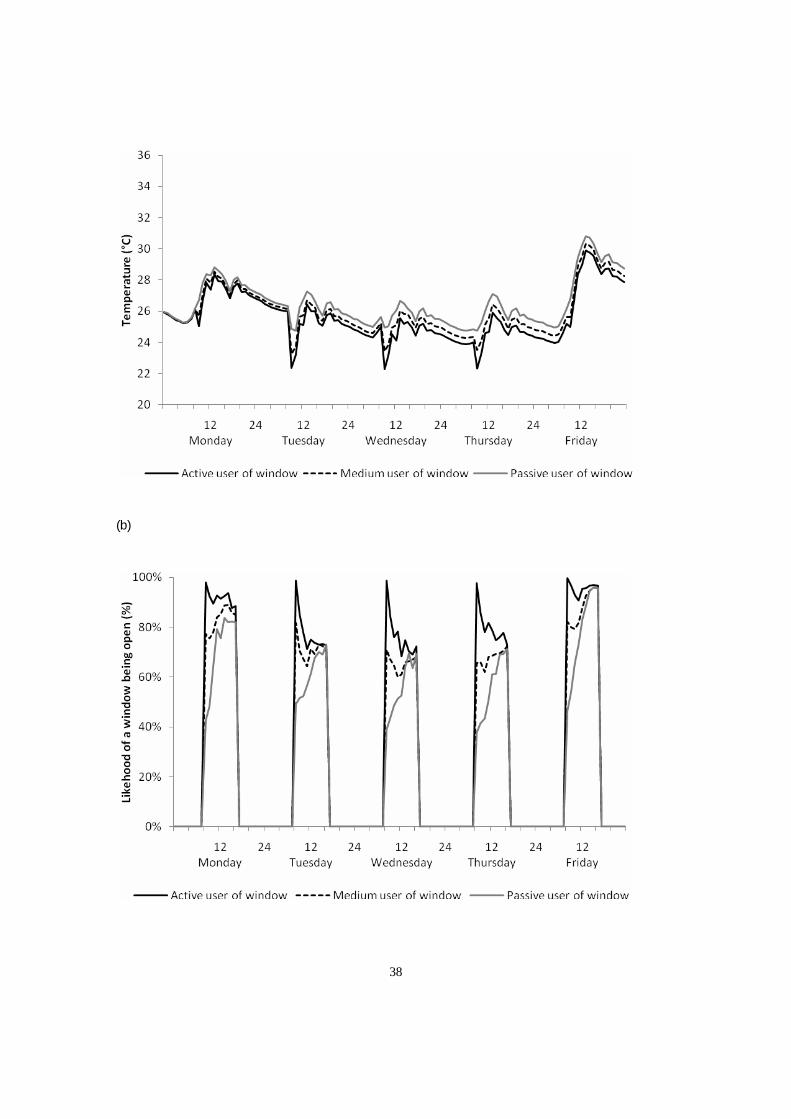
The models of manual window control in this study enable different window use patterns to be considered

in the prediction of indoor thermal conditions (Figure 8). Figure 8b shows the wide variation in window-

control patterns as a function of active, medium and passive user behaviour models. The average likelihood

of a window being open on arrival is 99% for the active window user, 76% for the medium window user,

17

43% for the passive window user. During the subsequent occupation periods the figures are 83% for the

active window user, 75% for the medium window user, 67% for the passive window user.

It is clear that individual differences in the interaction with a window play an important role in building

thermal performance (Figure 8a). The operative temperature inside an office, where an occupant most

actively controls the window in response to the intensity of indoor thermal stimulus, remains the lowest,

while the room temperature for the passive user of a window is the highest. The temperature of an office of

an active user of a window is up to 2.64C lower than that for a passive user of a window. The largest

difference between the two cases occurs at one hour after the occupant arrival on Wednesday. The

likelihood of a window being open at this simulation time step is 84% for the active window user and 44%

for the passive window user. As the weather conditions and internal heat gains remain the same between

the two cases, the temperature difference results from the difference in the window-control patterns of

occupants. The mean temperature difference between the two offices during occupied period is 1.15C.

5.4 Effects of thermal mass and occupant behaviour

Figure 9 demonstrates the variation in indoor temperature distribution as a function of light, medium and

heavy-weight construction with the medium user behaviour model of window-control. The results show

that the thermal responses of a light weight structure are most sensitive to the change in heat gains and

weather conditions. On average, the temperature in a light-weight office during occupancy is 1.75C higher

than that in a heavy-weight office.

As identified by Baker [36], the appropriate use of heavy or medium thermal mass and its effective

distribution in a building is an effective design strategy to moderate the extremes of thermal conditions.

Thermal mass combined with solar shading, night cooling and good ventilation is recommended design

practice for maintaining comfortable summer temperatures [4, 37]. The maximum and minimum office

18

temperatures among the three offices analysed are all observed in a light weight office. The maximum

temperature of 34.28C (at 2 pm on Friday) and the minimum temperature of 22.79C (at 10 am on

Tuesday) occur for the light-weight office. The largest temperature difference of 5.14C between light and

heavy-weight offices happens at 2 pm on Friday.


5.5 Fixed ventilation rate methods and occupant behaviour models of window-control

Figure 10 compares indoor temperature results obtained using the Yun algorithm with those obtained using

a fixed ventilation rate. It suggests, as expected, that the simplified fixed ventilation rate representation of

window-control does not well represent the variation experienced in the performance of natural ventilation.

An ac/h of 10 or higher is commonly applied in evaluation of summer temperatures [4] which would in this

case give predicted indoor temperatures even lower than for the 6 ac/h results shown here which could lead

to an underestimate of the actual room temperatures that would be experienced in practice.

It should be mentioned that the window-control activities, ventilation rates from an open window and

cooling effects of natural ventilation are dependent on various factors such as wind speed and direction,

ambient temperature, indoor thermal conditions and the detailed design of a window system. These factors

are not explicitly accounted for when fixed ventilation rates are assumed. Thus, a detailed simulation

incorporating user behaviour, ventilation paths and local climate conditions as carried out in this study has

potential to provide more robust prediction of the airflow rate and the thermal performance of naturally

ventilated buildings.


19

5.6 Comparative simulation with the Humphreys model

The research team led by Fergus Nicol and Michael Humphreys have recently proposed the Humphreys

algorithm for window opening in naturally ventilated buildings [10,11]. This algorithm is based on window

opening being an adaptive response to thermal discomfort and has also been implemented in ESP-r. As a

comparison to the new algorithm (the Yun algorithm) developed in this work and described in earlier

sections, the same office was simulated but with the Humphreys algorithm controlling the window opening

behaviour. The Humphreys algorithm [10] is also stochastic and it has a thermal comfort ‘dead-band’

which could be viewed as having the effect of making the probability of a window change event dependent

on the previous setting of the window as the window setting from the previous time step directly affects the

thermal comfort conditions of the current time step. Unlike in previous studies using the Humphreys

algorithm, here a Monte Carlo approach was employed to generate a statistical distribution. The results for

this application of the Humphreys algorithm are shown in Figure 10a. In general the operative temperature

ranges predicted are similar for both the Yun (22.2C to 30.8C) and Humphreys (24.4C to 30.2C)

algorithms as both predict the windows will generally be open for this warm period. However differences

between the two algorithms are also highlighted particularly with respect to the predicted behaviour on the

cooler days of the week. On these days the Humphreys algorithm predicts that the occupants will be

comfortable on arrival and will not open the windows until outdoor temperature, solar and internal gains

cause the internal temperature to exceed the comfort band and the occupant experiences some mild thermal

discomfort. This occurs around 11am for the more moderate Tuesday, Wednesday and Thursday conditions

in this example. This behaviour is shown in the increasing trend in the operative temperature for the

mornings of these cooler days which is opposite to the prediction from the Yun algorithm where window

opening on arrival causes the office temperature to drop initially due to the influx of cooler outside air. On

days where the room temperatures have already exceeded the Humphreys comfort band by arrival time then

the performance of the two algorithms is more consistent (Monday, Friday). Figure 11b shows the average

value for the probability function calculated in the Humphreys algorithm. The Humphreys algorithm has

been assigned a value of 0 when the comfort band is not exceeded (i.e. a window is closed). In comparison

20

to the earlier chart (Figure 11a) for the Yun algorithm, it can be seen that while in general the maximum

probabilities for the window being open on each of the days are similar the difference in predicted

behaviour on arrival is again highlighted.


6 Discussion

This study reports the development of a behavioural algorithm of manual window-control (i.e. the Yun

algorithm) using Markov chain and Monte Carlo methods from a longitudinal monitoring campaign and its

implementation into a dynamic energy simulation tool, ESP-r. The Yun algorithm generates a time series

of window states as a function of the indoor thermal stimulus, the previous window state and time of day in

order to simulate occupant behaviour of window-control observed in the monitoring campaign. Thus, the

algorithm would potentially contribute to more realistic predictions of thermal performances of naturally

ventilated buildings, compared with conventional simulation methods which deal with the use of windows

based on certain assumptions such as a predefined schedule, fixed ventilation rate and threshold method.

These assumptions are often without evidence from the field and attributed to discrepancy between

predicted and actual building performance [10]. We envisage that the application of the Yun algorithm in

dynamic simulation processes would allow us to better understand the roles of occupant behaviour in

building performance and develop more reliable and robust design strategies.

The Yun algorithm classifies building occupants into active, medium and passive users of windows and is

capable of quantifying the effects of the difference in occupant interactions with windows on thermal

performances. This study also provides evidence that the effects of occupant behaviour of window-control

patterns can be of the same order as the influence of thermal mass. The mean variation in indoor

temperature is 1.75C due to the different construction types and the variation caused by different user

behaviour of window-control is 1.15C. This also suggests that taking account of occupant behaviour in

building simulation tools is essential to ensure the accuracy and reliability of their simulation results.

21

Another outcome of this study is the comparison of the Yun algorithm with the Humphreys adaptive

algorithm of manual window-control. The two algorithms result in generally similar prediction results. The

differences in indoor temperatures between the algorithms over the occupied hours are in most cases less

than 0.5C. Particularly the temperature difference is minimal during the warmer days of the week

(Monday and Friday) when the indoor temperatures by the occupant’s arrival time of day go already over

the comfort band in the Humphreys algorithm.

The Humphreys algorithm was based largely on a 12 building survey (6 Aberdeen, 6 Oxford) carried out in

the 1990s. Buildings covered Educational, Local Authority and Commercial offices of both cellular and

open plan office types. Longitudinal and transverse studies were carried out [10]. The observations were

made only 4 times per day. Building fabric and building locations were varied. The Yun algorithm is based

on more comprehensive and more frequent observations across a smaller number of observation sites and a

narrower range of buildings and occupations. The Humphreys algorithm as it was published and evaluated

here does not distinguish between arrival times and later times of day. This may have been influenced by

factors such as the four-a-day sampling period, the occupant activities, the surrounding environments etc.

The thermal comfort basis for the Humphreys algorithm is not sensitive to non thermal factors such as

‘stuffiness’, contaminants, odours or other hypothetical desires for air movement or freshness. Sources of

‘poor air’ that could trigger non thermal window opening could possibly include high levels of dust, IT

equipment left running overnight, building materials that emit contaminants, odours, low humidity, un-

emptied bins containing organic materials, toilets, cleaning materials, etc. These non thermal triggers could

alter window opening behaviour and tend to increase window opening with (in the UK climate) some

associated increase in energy use for the enhanced ventilation rates in winter time and possibly some

reduction in peak summer temperatures [11].

22

Monitoring data that forms the basis of the Yun algorithm may be influenced by the specific situational and

contextual factors of the offices on campus such as pleasant surroundings (visual and aural), single

occupancy, easily operable windows, educational employee types etc. These may lead to enhanced window

use in these monitored offices. The educational employees in a campus setting may routinely open the

windows because it is pleasant to do so. This will not always be the case (e.g. road noise outside) and other

situations may lead to windows remaining closed until some thermal discomfort is experienced.

The Yun algorithm similarly to the Humphreys algorithm, may not be directly sensitive to the other non

thermal factors which may drive window opening events although it may indirectly capture these by its

separate treatment of window opening events upon arrival. The Humphreys approach directly incorporates

adaptive thermal comfort criterion based on rolling mean external temperatures which is now included in

standards to be applied to free running buildings [4,38] while the Yun algorithm is dependent on internal

temperatures only. The Yun algorithm approach, of defining different user types may offer some

advantages in identifying the critical roles of occupant behaviour in naturally ventilated buildings,

similarly, the incorporation of time of day or event driven effects (i.e. arrival, occupied periods) has

advantages and better reflects the occupant window-control behaviours discovered in the monitoring

activities.

Future work can be carried out in a number of areas in order to make the methodology more robust. Further

surveys, algorithm development and validation studies should be carried out in order to answer the open

questions. Both Humphreys and Yun methodologies have merits and it is expected that further data

gathering and analysis may lead to a solution containing elements of both. Both methodologies lend

themselves to being embedded in building design software and would give advantages over current

standard methods for design of comfortable and low energy buildings. The simulation methodology

illustrated here has comprehended occupant window opening behaviour and its stochastic variability. Other

occupant behavioural models such as occupancy models, blind, shade and light use models [9] can also be

23

integrated in future with the window algorithms in dynamic simulation to more fully represent the occupant

experience and impact on comfort, energy use and carbon emissions. Other uncertainties in parameters such

as internal gains and building fabric (thermal bridges etc) should also be comprehended in the methodology

and combined with the occupant models in order to give a realistic range of building performance (comfort

and carbon) under realistic operational conditions at the design stage [35].

Comprehending occupant behaviour and its effect on energy is recognised as one area where simplified

models are weak. Dynamic simulation relies on the same assumptions of behaviour used in the simplified

models. There is scope for the current and future work in this field to both develop robust human behaviour

models for use in dynamic simulation and to improve the simplified methods.

7. Conclusions

A newly developed algorithm (The Yun algorithm) for occupant window-control behaviour including

Markov chains and Monte Carlo methods and its implementation in dynamic building software for potential

application to building design has been described in detail. The Yun algorithm applied to a naturally

ventilated office was used to illustrate the predicted effect of user behaviour on the summer thermal

performance for a range of different building constructions. It was shown that variation between active and

passive window user behaviour can have a significant effect on thermal performance, the difference

between active and passive window use behaviour being of the same order as the difference between low

and high thermal mass constructions. A comparison was made between the Yun algorithm results and the

results from the alternative Humphreys algorithm. The similarities and differences between the two

approaches are discussed and areas for further work identified. The algorithm has been implemented in

open source simulation software to facilitate its dissemination and adoption in other simulation software or

by other researchers. An argument is presented for the incorporation of occupant behaviour models in

building design.

24

References:

[1] EU, On the energy performance of buildings, Directive 2002/91/EC of the European Parliament, 2002.

[2] BRE, Standard assessment procedure for energy rating of dwellings, Building Research Establishment

Publication, 2005.

[3] CIBSE, TM37: Design for improved shading control, Chartered Institution of Building Services

Engineers, London, 2006.

[4] CIBSE, Guide A, Environmental design, 7th Edition, Chartered Institution of Building Services

Engineers, London, 2006.

[5] ESRU, www.esru.strath.ac.uk/Programs/ESP-r.htm, 2008.

[6] D.R.G. Hunt, The use of artificial lighting in relation to daylight levels and occupancy, Building and

Environment 14 (1) (1979) 21-33.

[7] C.F. Reinhart, Lightswitch-2002: a model for manual and automated control of electric lighting and

blinds, Solar Energy 77 (1) (2004) 15-28.

[8] G.R. Newsham, A. Mahdavi, I. Beausoleio-Morrison, Lightswitch: a stochastic model for predicting

office lighting energy consumption, Proceedings of Right Light Three, the Third European Conference on

Energy Efficient Lighting, Newcastle-upon-Tyne, 1995, pp. 60-66.

[9] D. Bourgeois, C. Reinhart, I. Macdonald, Adding advanced behavioural models in whole building

energy simulation: A study on the total energy impact of manual and automated lighting control, Energy &

Buildings 38 (7) (2006) 814-823.

[10] H.B. Rijal, P. Tuohy, M.A. Humphreys, J.F. Nicol, A. Samuel, J. Clarke, Using results from field

surveys to predict the effect of open windows on thermal comfort and energy use in buildings, Energy &

Buildings 39 (7) (2007) 823-836.

25

[11] P. Tuohy, H.B. Rijal, M.A. Humphreys, J.F. Nicol, A. Samuel, J. Clarke, Comfort driven adaptive

window opening behaviour and the influence of building design, Proceedings of the 10th International

IBPSA Conference Beijing, 2007.

[12] J.F. Nicol, I.A. Raja, A. Allaudin, G.N. Jamy, Climatic variations in comfortable temperatures: the

Pakistan projects, Energy and Buildings 30 (3) (1999) 261-279.

[13] M.A. Humphreys, Outdoor temperatures and comfort indoors, Building Research and Practice 6 (2)

(1978) 92-105.

[14] P.R. Warren, L.M. Parkins, Window-opening behaviour in office buildings, Building Services

Engineering Research & Technology 5 (3) (1984) 89-101.

[15] R. Fritsch, A. Kohler, M. Nygard-Ferguson, J.L. Scartezzini, A stochastic model of user behaviour

regarding ventilation, Building and Environment 25 (2) (1990) 173-181.

[16] J.F. Nicol, Characterising occupant behaviour in buildings: towards a stochastic model of occupant use

of windows, lights, blinds, heaters and fans, Proceedings of the 7th International IBPSA Conference,

International Building Performance Simulation Association, Rio, 2001.

[17] S. Herkel, U. Knapp, J. Pfafferott, A preliminary model of user behaviour regarding the manual

control of windows in office buildings, Building Simulation, 2005.

[18] S. Herkel, U. Knapp, J. Pfafferott, Towards a model of user behaviour regarding the manual control of

windows in office buildings, Building and Environment 43 (2008) 588-600.

[19] G.Y. Yun, K. Steemers, User behaviour of window-control in offices during summer and winter,

Renewable in a changing climate: Innovation in the built environment, CISBAT international conference

2007, EPFL, Lausanne, 2007.

[20] G.Y. Yun, K. Steemers, Time-dependent occupant behaviour models of window-control in summer,

Building and Environment, (In press, Undated).

26

[21] G.Y. Yun, K. Steemers, N. Baker, Natural ventilation in practice: linking facade design, thermal

performance, occupant perception and control, Building Research & Information 36 (2008) 608-624.

[22] G.F. Lameiro, W.S. Duff, A Markov model of solar energy space and hot water heating systems, Solar

Energy 22 (3) (1978) 211-219.

[23] S.L. Scartezzini, A. Faist, T. Liebling, Using markovian stochastic modelling to predict energy

performances and thermal comfort of passive solar systems, Energy and Buildings 10 (1987) 135-150.

[24] F. Bottazzi, T.M. Liegling, J.-L. Scartezzini, M. Nygard-Ferguson, On a Markovian approach for

modelling passive solar devices, Energy and Buildings 1991 (1991) 103-116.

[25] J. Tanimoto, A. Hagishima, State transition probability for the Markov Model dealing with on/off

cooling schedule in dwellings, Energy and Buildings 37 (3) (2005) 181-187.

[26] J. Tanimoto, A. Hagishima, H. Sagara, A methodology for peak energy requirement considering actual

variation of occupants’ behaviour schedules, Building and Environment 43 (4) (2008) 610-619.

[27] J. Page, D. Robinson, N. Morel, J.-L. Scartezzini, A generalised stochastic model for the simulation of

occupant presence, Energy and Buildings (2007).

[28] A.C. Cameron, P.K. Trivedi, Microeconometrics: methods and applications, Cambridge University

Press, Cambridge, 2005.

[29] M. Mitzenmacher, E. Upfal, Probability and Computing: Randomized Algorithms and Probabilistic

Analysis, Cambridge University Press, 2005.

[30] C.M. Grinstead, J.L. Snell, Introduction to probability, available at

http://www.dartmouth.edu/~chance/teaching_aids/books_articles/probability_book/pdf.html, Undated.

[31] J.L.M. Hensen, On the thermal interaction of building structure and heating and ventilation system,

PhD thesis, Technische Universiteit Eindhoven, 1991.

27

[32] H. Maisel, G. Gnugnoli, Simulation of Discrete Stochastic Systems, Science Research Association,

Chicago, 1972.

[33] J. Remund, S. Kunz, Metoenorm Version 5.1 Handbook, METEOTEST, 2004.

[34] K.J. Lomas, H. Eppel, Sensitivity analysis techniques for building thermal simulation programs,

Energy and Buildings 19 (1992) 21-44.

[35] I. Macdonald, P. Strachan, Practical application of uncertainty analysis, Energy & Buildings 33 (2001)

219-227.

[36] N. Baker, The irritable occupant: recent developments in thermal comfort theory, Architectural

Research Quarterly 2 (Winter) (1996) 84-90.

[37] EST, CE129: Reducing overheating - a designers guide, Energy Saving Trust, available at

www.est.org.uk/bestpractice, 2005.

[38] CEN, CEN 15251: Indoor environmental criteria for design and calculation of energy performance of

buildings, Comite Europeen de Normalisation, Brussels, 2007.

28

List of Figures

Figure 1. Representation of a time series of binary window states using Markov chain

Figure 2. Diagram of the Yun algorithm

Figure 3. Modelling image of a theoretical cellular office

Figure 4. Position of photocells in a cellular office

Figure 5. Change in indoor temperature from the value at the immediately preceding iteration as the

iteration proceeds

Figure 6. Comparison between predicted and monitored probabilities of a window being open

Figure 7 Effects of occupant’s window-control behaviour on indoor temperature in medium weight thermal

mass structure

(a) Indoor temperature with standard deviation using the medium user behaviour models of window-

control for the simulation period, along with the likelihood of a window being open

(b) Ambient conditions

Figure 8 Indoor operative temperatures in an office with medium weight construction mass as a function of

passive, medium and active user behaviour models of window-control

(a) Indoor operative temperatures

(b) The likelihood of a window being open (i.e. the ratio of the number of iteration when a window is open

to the total number of iteration)

Figure 9 Indoor temperatures in an office with light, medium and heavy weight construction using a

medium user behaviour model of window-control

29

Figure 10 Comparison of indoor temperature as a function of passive, medium and active user behaviour

models of window-control with indoor temperature with fixed ac/h of 2, 4 and 6 in an office with a

medium-weight construction

Figure 11 Comparison of the results between the Yun and Humphreys algorithms


(b) Likelihood of a window being open (i.e. the ratio of the number of iteration when a window is open to

the total number of iteration)

30

List of tables

Table 1. Transition probability functions: logistic regression coefficients for the user behaviour models of

window-control (SD refers to standard deviation)

Table 2. Internal heat gains during the occupied period

Table 3. Construction of light, medium and heavy-weight thermal mass offices (from outside to inside)

Figures:

Figure 1. Representation of a time series of binary window states using Markov Chain

31

Figure 2. Diagram of the Yun algorithm

32

Figure 3. Modelling image of a theoretical cellular office

33

Figure 4. Position of photocells in a cellular office

34

Figure 5. Change in indoor temperature from the value at the immediately preceding iteration as the

iteration proceeds

35

Figure 6. Comparison between predicted and monitored probabilities of a window being open

36

(a)

(b)

37

Figure 7 Effects of occupant’s window-control behaviour on indoor temperature in medium weight

thermal mass structure

(a) Indoor temperature with standard deviation using the medium user behaviour models of window-

control for the simulation period, along with the likelihood of a window being open

(b) Ambient conditions

(a)

38

(b)

39

Figure 8 Indoor operative temperatures in an office with medium weight construction mass as a function of

passive, medium and active user behaviour models of window-control


(b) The likelihood of a window being open (i.e. the ratio of the number of iteration when a window is open

to the total number of iteration)

40

Figure 9 Indoor temperatures in an office with light, medium and heavy weight construction using a

medium user behaviour model of window control

41

Figure 10 Comparison of indoor temperature as a function of passive, medium and active user behaviour

models of window-control with indoor temperature with fixed ac/h of 2, 4 and 6 in an office with a

medium-weight construction

42

(a)

(b)

43

Figure 11 Comparison of the results between the Yun and Humphreys algorithms


(b) Likelihood of a window being open (i.e. the ratio of the number of iteration when a window is open to

the total number of iteration)

44

Tables:

Logistic transition probability function

where is the probability of a window state

transition from i to j and is indoor temperature

Regression results

Time of day Occupant type State transition a (SD) b (SD) Arrival Active Closed to open -14.094 (9.195) 0.717 (0.428) Arrival Medium Closed to open -7.989 (1.856) 0.359 (0.080) Arrival Passive Closed to open -7.777 (4.292) 0.293 (0.183)

Subsequent Medium Closed to open -11.383 (2.669) 0.365 (0.108) Subsequent Medium Open to closed 3.748 (2.462) -0.289 (0.103)

Table 1. Transition probability functions: logistic regression coefficients for the user behaviour models of

window control (SD refers to standard deviation)

45

Gain/Floor area (W/m2) Selected heat gain in the model

Occupancy 12

Lighting 12

Small power 8

Table 2. Internal heat gains during the occupied period

46

Floor Thermal mass

Material Thickness (mm) Conductivity W/(m. ̊C) Density kg/m3 Specific heat J/(kg. ̊C) R (m2.K)/W

Heavy Heavy mix concrete

150 1.400 2100 653 0.11

Medium Heavy mix concrete

150 1.400 2100 653 0.11

Wilton 10 0.060 186 1360 0.17 Light Aerated concrete

block 100 0.240 750 1000 0.42

Air 200 0.17 Chipboard 20 0.150 800 2093 0.13 Wilton 15 0.060 186 1360 0.25 Ceiling Thermal mass


Heavy Heavy mix concrete

150 1.400 2100 653 0.11

Medium Heavy mix concrete

150 1.400 2100 653 0.11

Light plaster 10 0.160 600 1000 0.06 Light Aerated concrete

block 100 0.240 750 1000 0.42

Air 200 0.17 Mineral ceiling 15 0.030 290 2000 0.50 External wall Thermal mass


Heavy Cement screed 10 1.400 2100 650 0.01 Polyurethane foam 100 0.030 30 837 3.33 Light mix concrete 100 0.380 1200 653 0.26 Gypsum plaster 10 0.420 1200 837 0.02 Medium Cement screed 10 1.400 2100 650 0.01 Polyurethane foam 100 0.030 30 837 3.33 Aerated concrete

block 70 0.240 750 1000 0.29

Gypsum plaster 10 0.420 1200 837 0.02 Light Cement screed 10 1.400 2100 650 0.01 Polyurethane foam 90 0.030 30 837 3.00 Aerated concrete 50 0.160 500 840 0.31 Air 200 0.17 Light plaster 10 0.160 600 1000 0.06 Internal wall Thermal mass


Heavy Cement screed 10 1400 2100 650 0.01 Light mix concrete 100 0.380 1200 653 0.26 Gypsum plaster 10 0.420 1200 837 0.02 Medium Cement screed 10 1.400 2100 650 0.01 Aerated concrete

block 70 0.240 750 1000 0.29

Gypsum plaster 10 0.420 1200 837 0.02

47

Light Cement screed 10 1.400 2100 650 0.01 Aerated concrete 50 0.160 500 840 0.31 Air 200 0.17 Light plaster 10 0.160 600 1000 0.06 Table

yun, geun young and tuohy, p.g. and steemers, k. (2009

Documents