youth unemployment and crime: new lessons · pdf fileniknami and seminar participants at sofi....

1

YOUTH UNEMPLOYMENT AND CRIME:

NEW LESSONS EXPLORING LONGITUDINAL REGISTER DATA*

Hans Grönqvist

SOFI, Stockholm University

[email protected]

October 24, 2011

ABSTRACT

This paper investigates the link between youth unemployment and crime

using a unique combination of labor market and conviction data spanning the

entire Swedish working-age population over an extended period. The

empirical analysis reveals large and statistically significant effects of

unemployment on several types of crime. The magnitude of the effect is

similar across different subgroups of the population. In contrast to most

previous studies, the results suggest that joblessness explain a meaningful

portion of why male youths are overrepresented among criminal offenders. I

discuss reasons for the discrepancy in the results and show that that the use

of aggregated measures of labor market opportunities in past studies is likely

to capture offsetting general equilibrium effects. Contrary to predictions by

economic theory the effect of unemployment on crime is not mediated by

income. Instead, an analysis of crimes committed during weekdays versus

weekends provides suggestive evidence that unemployment increases the time

that individuals have to engage in crime.

Keywords: Unemployment; Delinquency; Age-crime profile

JEL: K42; J62

* This paper has benefitted from comments by Anders Björklund, Richard Freeman, Matthew Lindquist, Susan

Niknami and seminar participants at SOFI.

2

1. INTRODUCTION

The age pattern of crime is close to universal. In virtually all countries, criminal activity

rise with age, peak in the late teens, then fall (e.g. Hirschi and Gottfredson 1983). For

example, while the conviction rate among Swedish men aged 19 to 24 in the year 2005

amounted to 4.2 percent the corresponding figure for men aged 29 to 34 was nearly half

as large. A popular explanation for the age distribution of crime is that youths are more

exposed to unemployment (e.g. Freeman 1996; Grogger 1998). Economists have argued

that the income loss generated by unemployment lowers the opportunity cost of engaging

in crime (cf. Becker 1968; Ehrlich 1973). Others have hypothesized that joblessness

triggers frustration and anger, which in turn may lead to violent behavior (e.g. Agnew

1992). It has also been suggested that unemployment provides individuals with more

time and opportunities to commit crime (Felson 1998). Understanding the link between

youth unemployment and crime is not only important to help explain the age

distribution of crime but is also a key issue for public policy since any relationship

would indicate that the social benefits of investments in labor market programs may

exceed those usually claimed.

The aim of this paper is to empirically investigate the effect of youth

unemployment on crime. Although a large body of research has documented the

relationship between overall labor market opportunities and crime there are surprisingly

few studies on youths.1 Freeman (1999), Fagan and Freeman (1998) and Bushway (2010)

1 Past investigations of the relationship between overall labor market opportunities and crime

include: Entorf and Spengler (2000), Gould et al. (2002), Machin and Megihr (2004), Lin (2008),

Papps and Winkelmann (2002), Raphael and Winter-Ebmer (2001), Doyle et al. (1999), Cornwell

and Trumbull (1994). All of these studies use regional level panel data. In general, the results in

these studies suggest that a one-percentage-point increase in the unemployment rate increases

property crime by about 1–2 percent. The effect on violent crime is much smaller. Edmark (2005)

find similar results using Swedish data. One of the few studies employing individual level data is

Rege et al. (2009). The paper shows convincing evidence that involuntary job loss in Norway

induced by plant closures is associated with a 14 percent higher probability of being charged of a

crime. Unfortunately, since the research design requires the subjects to have stable employment

histories it is less suitable for studying youths who often have little or no previous job experience.

Another related literature that also uses individual level data examines at the effect of job

training programs and other labor market interventions on adult crime (e.g. Lattimore et al.

3

review the literature and concludes that there is a sizable negative correlation. There are

however several reasons to be concerned about the results in past studies. First, the

observed relationship between unemployment and crime is (at least partially) likely to

be spuriously driven by factors researchers have been unable to control for. Impatience

represents one such factor if individuals with high discount rates are more prone to

criminal activity and more exposed to unemployment (cf. DellaVigna and Paserman

2005). Joblessness could also be linked to consumption of various criminogenic goods; e.g.

alcohol and narcotics.2 Second, the literature has not been able to establish direction of

causality. One problem is that potential employers may react adversely towards

individuals with a criminal record (Grogger 1995; Kling 2006). A related issue is that

firms might choose to relocate as a consequence of rising crime rates (Cullen and Levitt

2005). If crime raises the risk of unemployment instead of the opposite this will bias the

results in past studies upwards. Third, due to data limitations most investigations have

relied on aggregated measures of unemployment and crime. In these models any effect of

unemployment on criminal behavior is likely to be confounded by general equilibrium

effects. For instance, in areas with high unemployment rates there may be fewer

resources available to steal and fewer potential victims on the streets (Mustard 2010).

Although some studies have tried to account for these problems no single study has been

able to properly address all issues.

The most convincing research to date use regional level panel data to control for

persistent unobserved regional factors. Fougère, et al. (2009) study a panel of French

regions and find a statistically and economically significant effect of youth

unemployment on property crime. Consistent with economic theory there is little or no

significant effect on violent crimes. Öster and Agell (2007) study a panel of Swedish

1990; Lalonde 1995 and Schoecht et al. 2008). Of these studies, Schochet et al. (2001) finds a

relative moderate decline in criminal activity for individuals randomly assigned to the Job Corps

program. 2 See e.g. Grönqvist and Niknami (2011) for evidence on the link between alcohol and crime.

4

municipalities observed during the 1990s and find no significant effect of youth

unemployment on crime. Only a few studies use individual level data. In general, these

studies find a stronger relationship (Freeman 1999). Grogger (1998) and Witte and

Tauchen (1994) show that employment and wages are significantly negatively correlated

with self-reported illegal behavior in the US. A key limitation in these studies is however

that the data used does not allow the researchers to account for unobserved

characteristics of the individuals.

In contrast to past studies, this paper uses individual level data from

administrative registers. The dataset covers the entire Swedish working-age population

and includes rich information on labor market, educational and demographic

characteristics of the individuals. The data have been merged to information on the

universe of convictions in Swedish courts from 1985 to 2007. Among other things there is

information on the type of crime as well as the exact date of the offense. The longitudinal

nature of the data makes it possible to disentangle the effect of unemployment from

many aspects of the individual using several identification strategies. My main approach

is to relate changes in unemployment to changes in criminal behavior. The advantage of

the strategy is that it eliminates all fixed unobserved characteristics of the individual.

One drawback is that the model excludes the possibility of controlling for the influence of

past criminal behavior (at least without imposing strong assumptions). I therefore

supplement the analysis with regressions that relate levels of crime to levels of

unemployment in which I condition on lagged crime. The benefit of both models is that

they are likely to produce estimates that come closer to having a causal interpretation

than what has been feasible in the previous literature. Comparing the results from two

models that rests on different assumptions also provides a way to corroborate the

findings.

5

This paper contributes to the literature by using data not previously available to

researchers.3 Coupled with an identification strategy that rules out many potential

confounding factors I am able to explore several new aspects of the question. First, no

previous study using individual level data has explicitly tried to account for unobserved

characteristics of the individual. Second, the data makes it possible to investigate

subgroups of the population with elevated risks of criminal involvement. The data

identify individuals with a criminal history, low cognitive skills, immigrant status, and

poor parental socioeconomic background. It is well known that these groups account for a

disproportionate share of total crimes committed (e.g. Levitt and Lochner 2001; Hällsten,

Sarnecki and Szulkin 2011). Learning about the extent to which worse labor market

prospects help explain criminal behavior in these groups could provide valuable

knowledge on how to optimally target labor market and educational programs. No past

investigation has ever separately studied population subgroups using a compelling

identification strategy. Third, the data allows me to disentangle some of the mechanisms

through which youth unemployment may affect crime. By using information on

disposable income it is possible to investigate whether the potential effect is mediated

via income, as suggested by economic theory. Moreover, if employment matters because

it incapacitates individuals so that they have less time to commit crime then the effect of

joblessness should be more pronounced for crimes committed during weekdays when

most individuals normally work. I examine this by exploiting information on the exact

date of the offense.4 Last, the use of individual data makes it possible to isolate the effect

of unemployment on the supply of criminals. This is important since it provides a cleaner

test of the economic theory of crime than what can be achieved using aggregated data.

3 Only a few studies have ever used population conviction data to study crime. One exception is

Hjalmarsson and Lindquist (2010) who use similar Swedish crime data to investigate the

intergenerational association in crime. 4 This strategy was first adopted by Rege et al. (2009).

6

Unemployment is found to have a small and statistically significant effect on

violent crime and a sizable effect on financially motivated crimes: being unemployed for

more than six months increases the likelihood of committing a violent crime by about 2

percent and raises the probability of committing theft by about 33 percent. I also find

large and significant effects on drug offenses as well as drunken driving (DUI).The

impact of joblessness on overall crime constitutes almost one quarter of the crime gap

between 19 to 24 year olds and individuals aged 29 to 34. This result suggests that

unemployment may explain a meaningful portion of why male youths account for a

disproportionate share of total crime. There is also a clear dose-response relationship in

the sense that the risk of crime is increasing in the time spent in unemployment. The

estimates are similar across different subgroups of the population. In contrast to the

predictions by economic theory the effect is not mediated via income. Instead, an

analysis of crimes committed during weekdays versus weekends provides tentative

evidence that unemployment increase the time and opportunities that individuals have

to engage in crime. The analysis further shows little evidence that the adverse effects of

unemployment persist over time.

My findings partly contradict those in the previous literature using aggregated

data that in general finds smaller effects. One possible explanation is that the use of

aggregated data has prevented past investigations to identify pure behavioral responses

to unemployment. This view is supported by an auxiliary analysis where I collapse the

individual level data by county and year.

The paper is outlined as follows. Section 2 provides a brief background to the

Swedish criminal justice system and gives some facts about youth crime in Sweden.

Section 3 discusses the data and research design. Section 4 presents results from the

analysis and Section 5 concludes.

7

2. SWEDISH JUSTICE SYSTEM AND UNEMPLOYMENT BENEFITS 5

The Swedish crime rate is high compared to many other countries. In the year 2006 the

total number of assaults per 100,000 inhabitants reported to the police was 845. The

same year official crime statistics show that 787 assaults per 100,000 inhabitants were

recorded by the US police and the corresponding number for Canada is 738 (Harrendorf

et al. 2010). Even though these figures partly reflect differences in the propensity to

report crime, differences in crime severity and inconsistencies in crime definitions the

rates are comparable across many types of crimes where underreporting is likely to be

similar. For instance, in 2006 the burglary rate per 100,000 persons in Sweden was

1,094. In the US the burglary rate was 714 and in Canada the rate amounted to 680

recorded cases per 100,000 inhabitants.

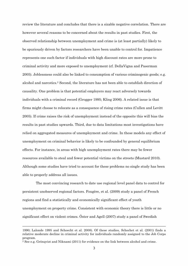
As previously mentioned, youths represents the most criminally active age

group in Sweden. Figure 1 shows the share of convicted persons in 2005 by age relative

to national conviction rates. A number above (below) one indicates that the share of

convicted persons for that age group is higher (lower) than the average for all age

groups. As can be seen the relative overall conviction rate peaks already before age 20,

then falls. Note that the share of convicted persons has dropped to the average for all

ages as early as age 29. Figure 1 also shows that the age distribution of theft is even

more heavily skewed to the right. However, there is no clear age-crime profile for violent

crimes. It is worth mentioning that these findings hold irrespective of the type of crime

data used (cf. Swedish National Council for Crime Prevention 2007).

In Sweden, the general courts deal with both criminal and civil cases. The

general courts are organised in a three-tier system: district courts, courts of appeal and

the Supreme Court. The district court is the court of first instance. Criminal cases are

normally instituted when a public prosecutor initiates prosecution proceedings against a

5 This section primarily draws on Axelsson (2010).

8

suspect by submitting an application to a district court. The court rules on cases after a

main hearing attended by both parties, who state their claims and other circumstances

relating to the case. Criminal cases are normally tried by one judge and three lay judges.

Those who lack the economic means to take advantage of their rights are entitled to

public legal aid. The age of criminal liability is 15. All individuals above this age are

treated in the same juridical system. Some special rules does however apply for

juveniles. For instance, cases involving youths are to be dealt with promptly.

The Swedish unemployment insurance is voluntary income-related for members

of unemployment insurance funds. The benefits are proportional to previous income up

to a ceiling but there is supplementary compensation through collective agreements. The

maximum duration of benefits is 300 days. However, the rules allow for re-qualification

through participation in active labor market programs for workers at risk of benefit

exhaustion. In order to be entitled for unemployment benefits an individual is required

to have worked for 4-6 months during the past 12-mont period. Since 1992 the

replacement level for most of the workers has been around 80 percent which is relatively

large in comparison to many other developed countries. Individuals not entitled to

unemployment benefits are confined to social assistance.

3. DATA AND EMPIRICAL STRATEGY

3.1 Data and sample selections

This study uses data from various administrative registers collected and maintained by

Statistics Sweden. The data span the entire Swedish population aged 16 and above each

year 1985 to 2007 and include information on a wide range of labor market, educational

and demographic characteristics. The dataset was augmented with information on all

convictions in Swedish district courts during the period. Among other things there is

information on the type of offense and the sentence ruled by the court. Date of offense is

9

known in about 70 percent of the cases. There is however some measurement error in

this variable since the exact date of the crime is not always known (e.g. a burglary that

is not discovered before the owner returns home from her holidays). In these cases the

court makes an educated guess about the crime date. One conviction may include several

crimes and I observe all crimes within a single conviction. Speeding tickets, and other

minor offenses are not included in the data.

The crime categories of interest in this paper are: (i) Any crime; (ii) Violent crimes;

(iii) Theft; (iv) Drug offenses; (v) Drunken driving (DUI). All of these categories represent

common types of crimes in Sweden. Table A.1 describes the exact way in which these

variables have been constructed.

My main sample includes male youths aged 19 to 25 with at least one recorded

unemployment spell. 6 The period of observation is from 1992 to 2005. The sample

contains 723,392 individuals. The reason for not including younger individuals is that

most youths below this age are enrolled in upper secondary school.7 Information on

employment status is further only available from 1992. To allow for a lag between the

date of the crime and the conviction I choose to end the observation period in 2005.

In the analysis I separate between how many days an individual has been

unemployed during the year. More specifically, I create dummies for if the individual has

been unemployed 1-90 days, 91-180 days, and more than 180 days. It is plausible to

think that the risk of crime should increase with the time spent in unemployment. Long-

term unemployed will have had more time to engage in crime and have experienced

greater reductions in legal income compared to short-term unemployed. Only a few

previous studies have attempted to quantify the relationship between unemployment

duration and crime (Good et al. 1986; Thornberry and Christenson 1986).

6 To be registered as unemployed an individual needs to report to the state employment office.

Unemployment benefits are contingent on having registered. 7 In Sweden, more than 95 percent of all individuals continue immediately to upper secondary

school. Most of the students who graduate do so at age 19.

10

I include a set of standard individual background characteristics in the analysis:

high school graduation, family size, marital status, age, and immigrant status.

Information on disposable income and annual earnings is used to test the prediction by

economic theory that the main reason for why unemployment matters is because it

generates a loss of income (e.g. Freeman 1999). The data further contain an exact link

between children and their biological parents. It is therefore possible to add information

each parent’s highest completed level of education. Parental education is observed the

year the child turns 16. At this age most parents have completed their education. In the

data there is also information on compulsory school grades for children who finished

school during the period 1988 to 2007. I include the grade point average (GPA) in the

analysis as a combined measure of cognitive skills and ambition. To account for changes

in the grading system over time as well as potential grade inflation I compute the

percentile ranked GPA by year of graduation.

Table 1 presents descriptive statistics for selected variables. To see how well the

results are likely to generalize to the whole population of male youths, summary

statistics is shown both for my main sample and for all males aged 19 to 25. Comparing

the numbers in column (1) to those in column (2) it is clear that my sample is slightly

disadvantaged compared to the entire population of male youths: the share convicted

persons is higher (5.2 versus 4.2 percent), percentile ranked compulsory school GPA

lower (39 versus 43), and parental education poorer; although the latter difference is

small. Not surprisingly, the average number of days spent in unemployment is higher

and mean disposable income lower.

Data on criminal behavior is in this paper inferred from register information on

convictions. The main advantage of administrative data compared to self-report data is

that the latter is known to be plagued by underreporting and measurement error

(McDonald 2002). The large samples available in administrative registers also increase

11

statistical precision. However, conviction data are not flawless. Criminal behavior is only

observed for individuals who have been convicted in court. One concern is that people

with worse labor market opportunities may be more likely to get convicted conditional on

actually having committed a crime. This is the case if, for instance, jobless individuals

are more likely to get caught or have fewer resources available for defense at a criminal

trial. This is a caveat important to bear in mind when interpreting the results. Note

however that this is only a problem if this kind of selection is not picked up by the

control variables.8 Recall that my empirical strategy accounts for all permanent

unobserved heterogeneity in addition to time-varying factors. Moreover, the analysis

focuses on a sample of individuals where everyone becomes unemployed at least once.

This means that the sample is homogenous in the sense that the only difference between

individuals is the timing of the onset of the unemployment spell. If the criminal justice

system treats individuals with elevated unemployment risks similar then the problem is

less severe in this population.

3.2 Research design

As discussed earlier, any investigation of the link between unemployment and crime

needs to consider potential omitted variables and reverse causation. Studies using

aggregated data are plagued by additional problems associated with general equilibrium

effects. Although individual level data account for the last problem it is important to also

deal with the first issues.

The longitudinal nature of the data allows me to take one important step in the

direction towards identifying the causal effect of joblessness on crime. My main analysis

is based on the following regression model

8 In their study of the effect of education on crime as measured by arrests Lochner and Moretti

(2005) raises a similar concern. Using data on self-reported crime they conclude that for this to be

a problem education must substantially alter the probability of being arrested conditional on

criminal behaviour.

12

(1)

where i and t denotes individual and year, respectively. is an indicator set to

unity if the individual has committed crime during the year and zero otherwise.

Unemployment is measured with three dummies for if the individual has been

unemployed for a given number of days during the year. is a vector controlling for

time-varying variables; is a set of individual fixed effects; is a set of year fixed

effects; and is an error term. The main parameters of interest in this model are

. Each parameter provides the effect on crime of being unemployed for d

number of days relative to individuals that have not yet started (or just ended) their

unemployment spell. Since it is reasonable to assume that the probability of committing

crime is increasing in the time spent in unemployment I expect that .

The individual fixed effects absorb all individual characteristics that are persistent

over time regardless whether these are observed or not. Some persons may, for instance,

be less patient by nature, which could make them less likely to invest in work and at the

same time more likely to engage in crime (e.g. Lochner and Moretti 2005). Another

potential omitted factor is ability (e.g. Levitt and Lochner 2001). The year fixed effects

controls for time-varying factors that affect all individuals in the same way. This could

be cuts in governmental spending or macroeconomic events.

The model assumes that the error term is mean zero conditional on past, current

and future values of the regressors, i.e. that for all t. This

assumption is violated if unobserved individual shocks correlates with an individual’s

employment status and risk of crime. Controlling for individual characteristics that

change over time alleviates this problem but does not remove it. The assumption is also

corrupted if past factors linked to crime affect unemployment today and are not captured

by the control variables. One issue that in has been raised in the literature is the

13

possibility that employers discriminate between individuals with a criminal record (e.g.

Grogger 1995, Kling 2006). Fortunately, I am able to address this matter by estimating

regressions that controls for lagged crime. The model is specified as follows

(2)

Under the assumption that controlling for past criminal behaviour (and other covariates)

captures all unobserved factors that are correlated with unemployment and crime, i.e.

, the ordinary least squares

(OLS) estimator will consistently estimate . Also this supposition could be

questioned. Nevertheless, the benefit of the model is that it provides a way to

corroborate the findings.9 Although no single model will identify the causal impact of

youth unemployment on crime both models are likely to produce estimates that come

closer to having a causal interpretation than what has been possible in the previous

literature.

4. RESULTS

4.1 Main results

This section presents the results from my empirical analysis of the effect of youth

unemployment on crime. My baseline specification, given by equation (1), relates

changes in an individual’s probability of committing crime during the year (for which he

later was convicted for) to changes in the number of days spent in unemployment. I also

present results from regressions controlling for the lag of the dependent variable. To

9 It is also possible to estimate fixed effects models that include lagged outcomes. However, in this

model the residual will be mechanically correlated with the lagged dependent variable causing

the OLS estimator to be biased (Nickell 1981). Although there are methods to estimate such

models (e.g. Arellano and Bond 1991) they rely on rather strong assumptions of the data

generating process.

14

conserve space I suppress the coefficients of the control variables (available on request).

In general, these show a significant increased risk of crime for individuals that have not

completed high school, immigrants, individuals with lower compulsory school GPA, past

offenders, and individuals with worse parental socioeconomic background. The standard

errors are clustered at the individual level to account for arbitrary serial correlation and

heteroscedasticity.

Before proceeding to the main results it is useful to illustrate the raw correlation

between unemployment and crime. For this purpose Table 2 presents pooled OLS

estimates. Panel A contains estimates from regressions that only control for year and

age. Panel B adds further covariates: dummies for high school graduation, county of

residence, foreign-born, crime in the past two years, married, divorced, each parent’s

highest completed level of education, number of children (linearly), and compulsory

school GPA (linearly).

In column (1) of Panel A it is clear that there is a sizable correlation between

unemployment and criminal behavior. Being unemployed between 1 and 90 days is

associated with a 1.93 percentage point increased risk of committing crime. In relation to

the mean of the dependent variable this translates into a 37 percent (.0193/.0527) higher

probability of engaging in crime. The magnitude of the effect is increasing in the number

of days spent in unemployment. Individuals who have been unemployed for more than

180 day are 6.19 percentage points more likely to commit crime. Due to the large sample

size the statistical precision is high and all estimates are significant well below the one

percent level. The same is true for the F-test of joint significance of the unemployment

coefficients. A similar pattern is visible in columns (2) to (5). For all types of crime there

is a strong and statistically significant relationship between joblessness and the

likelihood of committing crime. There is also a clear dose-response relationship.

15

As can be seen in Panel B, adding a rich set of covariates to the regressions

renders the size of most of the coefficients to cut in half. The finding highlights the

importance of accounting for omitted individual characteristics. In all cases except for

drug offenses the dose-response relationship prevails.

Even though the regressions control for a large number of covariates it is still

likely that unobserved individual characteristics biases the OLS estimator. To the extent

that these characteristics are constant over time the individual fixed effects estimator

will control for this. Table 3 presents the regression output based on equation (1).

Comparing these estimates with the pooled OLS estimates in Panel B of Table 2 we can

see that the coefficients are further reduced. In general, the estimates in Table 3 are

about one third as large. Being unemployed between 1 and 90 days is found to increase

the probability of committing any type of crime by about .03 percentage point. The

results also show that being unemployed for more than 180 days quadruples this risk.

Relative to the sample mean long-term unemployed individuals (>180 days) are about 22

percent (.0120/.0527) more likely to engage in crime. In column (2) we can see that the

magnitude of the effect is smaller for violent crimes. Long-term unemployment is found

to raise the risk of violent crimes by .05 percentage points, or stated differently, by just

below 2 percent (.0005/.0260). As can be seen in column (3), the effect is substantially

larger for theft. Long-term unemployment increases the likelihood of committing theft by

.46 percentage points, or by 33 percent (.0046/.0138).

The difference between the estimates in columns (2) and (3) is striking and the

result is consistent with economic theory which suggests that the effect should be

stronger for financially motivated crimes. Columns (4) and (5) also show large effects of

unemployment on drug offenses and DUI. To the extent that financial resources are

necessary to buy alcohol and narcotics, the fact that such offenses increase when people

are without job also suggests that financial constraints may be an important

16

determinant of delinquency. However, since the mean of the dependent variables are

quite low, and substance use could itself affect the risk of being unemployed, the results

should be interpreted with caution.

For sake of comparison Panel B also displays estimates from regressions using a

continuous measure of days in unemployment. Evaluated at 100 days of unemployment

the results reveal a .05 percentage point higher probability of committing any type of

crime.

To better understand the magnitude of the coefficients it is useful to compare

the estimates to other known determinants of criminal behavior. Ability represents one

such factor (e.g. Freeman 1996; Levitt and Lochner 2001). In my sample, the crime gap

between individuals who scored above versus below the median in the compulsory school

GPA distribution is 5.63 percentage points (.0767-.0204) (cf. Table 5). The effect of long-

term unemployment on crime constitutes roughly 20 percent of this gap (.0120/.0563).

Repeating this exercise for violent crimes and theft I find that the effect of long-term

unemployment constitutes about 1.6 (.0005/.0563) and 27 (.0046/.0563) percent of the

crime gap between these groups, respectively.

Another way to grasp the size of the effect is to relate it to the age-crime profile.

In 2005 the conviction rate for male youths aged 19 to 24 was 4.2 percent. The

corresponding number for males aged 29 to 34 was 2.2 percent. The same year the share

of individuals aged 19 to 24 who experienced at least 180 jobless days was 9.3 percent

and the analogous figure for 29 to 34 year olds is 4.1 percent. The results in this paper

suggests that long-term unemployment account for almost one quarter (.0120/(.093-

.041)) of the crime gap between these groups. This is by all measures a substantial effect.

One concern with the individual fixed effects model is that it does not account

for the potential influence of past criminal behavior on current employment status. To

investigate this I estimated regressions controlling for lagged crime; cf. equation (2). The

17

results are presented in Table 4. The size of the coefficients is higher for all types of

crimes compared to the estimates in Table 3. For instance, long-term unemployment is

found to raise the probability of committing any type of crime by 2.89 percentage points.

When placed in relation to the sample mean the estimate suggest a 55 percent

(.0289/.0527) increase in the risk of crime. Aside from being larger the overall pattern of

the estimates is similar to that in Table 3: clear indications of a dose-response

relationship; and substantially smaller effects for violent crime. It is also worth

mentioning the huge predictive power of lagged crime, especially for violent crimes.

4.2 Is the effect different for high risk individuals?

Having demonstrated that the effect of joblessness triumph different identification

strategies I next ask whether the relationship is stronger in subgroups of the population

at higher risk of criminal involvement. I examine this by estimating separate regressions

for each subgroup. The results are shown in Table 5. To conserve space I only present

estimates for the linear measure of unemployment duration; however, the results are

similar when relaxing functional form by using dummies. All reported coefficients and

standard errors are scaled up by a factor 100. Numbers in italics show sample means.

For comparison purposes, the first row shows the baseline estimates presented in Table

3.

I start by examining individuals that differ in terms of criminal history.

Criminal background is defined as having committed any type of crime in the past two

years. Comparing the estimates for past offenders to those of persons with no criminal

background we can see that the estimates are larger in the former group. Evaluated at

100 days of unemployment, the coefficient suggests a 2.14 percentage point increase in

the probability of committing any type of crime for past offenders and a .45 percentage

point increase for subjects with no criminal background. However, when compared to the

18

mean of the dependent variable the magnitude of the effect is quite similar: a 9 and a

12.2 percent increase in the risk of crime, respectively. The pattern holds also for the

other types of crime.

I proceed by comparing the effect size between foreign-born individuals and

native Swedes. It is well-known that immigrants are overrepresented among criminal

offenders (Hällsten, Sarnecki and Szulkin 2011). This is confirmed by looking at the

sample means. The results reveal that the magnitude of the unemployment effect is

bigger in absolute terms for foreign-born than for natives. 100 days of unemployment is

found to raise the risk of crime among immigrants by about .94 percentage points. For

natives this results show a .43 percentage point increase; although, in relative terms the

results are again similar across groups.

Table 5 also hosts results from separate analyses by parental education. Low

educated parents is defined as no parent having attained education beyond the

compulsory school level. High educated parents is defined as at least one parent having

graduated from high school or more. For most types of crime there is a positive and

statistically significant effect of time spent in unemployment on the probability of

engaging in crime. In nearly all cases the estimates are however not statististically

distinguishable across the groups.

Last, I investigate possible heterogenous effects with respect to compulsory

school GPA. It turns out that the magnitude of the impact is greater for individuals with

compulsory school GPA below the median. Still, the relative effect sizes are quite similar

across the groups.

In summary, the results in this subsection suggest little evidence that the

effects of joblessness are in particular subgroups of the population.

4.3 Extensions

19

So far, the results presented in this paper suggest that unemployment is adversely

related to crime. This subsection attempts to disentangle some of the mechanisms that

have been proposed in the literature as explanations of the unemployment-crime link. I

also provide evidence on the potential dynamic impact of joblessness on crime.

4.3.1 Mechanisms

Standard economic models of crime suggest that an individual chooses whether or not to

engage in crime based on the expected returns to legal and illegal activities (e.g. Becker

1968, Ehrlich 1973). The model implies that joblessness may induce people to commit

crime because it lowers an individual’s expected legal income prospects. The model also

implicitly suggests that any effect on crime is likely to be more pronounced for crimes

that are associated with financial gain. The results presented in this paper showing

much stronger effects of unemployment on theft compared to violent crimes indeed

support the economic theory. This finding has also been documented in many previous

studies using aggregated data as well as in individual level studies. For instance, in

their analysis of low-income British youths Farrington et al. (1986) finds that the

significant increases in crime occurring during periods of unemployment relative to

periods of employment was isolated to offenses involving financial gain. The empirical

regularities are supported by anecdotal evidence based on interviews with burglars

which suggests that credit constraints were an important factor behind the decision to

engage in crime (Wright and Decker 1994).

Since my data include detailed information on income it is possible to probe

deeper into this issue. I started by quantifying the effect of unemployment on disposable

income by re-estimating equation (1) with the only exception that income was used as

dependent variable (available on request). It turns out that long-term unemployment is

associated with 17 percent lower disposable income and 73 percent lower annual

20

earnings. The difference in the estimates is due to various social transfers following

joblessness.

Having documented the “first-stage” relationship between joblessness and

income I then estimated equation (1) controlling for disposable income. If the income loss

is the main driving force behind the unemployment-crime relationship one would expect

to find the estimates in Table 3 to fall when including income as a regressor. Note

however that the results from this exercise should be interpreted with caution since

income cannot be considered as a predetermined variable. In Table 6 we can see that the

coefficients are virtually unchanged when controlling for disposable income. This result

suggests that the income mechanism might not be as important as emphasized in the

literature.

It has also been suggested that employment mechanically incapacitates

individuals thereby preventing them to commit crime (Felson 1998). Both Luallen (2006)

and Jacob and Lefgren (2003) demonstrate the importance of incapacitative effects in the

context of schooling. If true, then unemployment will increase the time and opportunities

that individuals have to engage in illegal behavior. Rege et al. (2009) tests this

mechanism by separately investigating crimes committed during weekdays versus

weekends. If there is an incapacitation effect of employment then one would imagine

that the impact of unemployment on crime is stronger during weekdays when most

individuals normally work. The results in Rege et al. show that unemployment caused by

involuntary plant closures in Norway indeed leads to more crime during weekdays

compared to weekends.

I investigated this mechanism by extracting information on the date of the

offense which allowed me to identify whether the crime was committed on a weekday or

weekend. Since the mean of the dependent variable already is low for some types of

crime the analysis was only possible for overall crime. The results are presented in Table

21

7. The point estimate in column (1) show that 100 days of unemployment leads to a .46

percentage point increase in the probability of committing crime on a weekday. The

coefficient in column (2) suggests smaller effect for weekend crimes: being unemployed

for 100 days is associated with a .17 percentage point increase in the likelihood of

engaging in crime on a weekend. Also when compared to the sample mean the effect is

stronger for weekday crimes. The probability of committing weekday crimes increases by

about 12.5 percent (.0046/.0388) whereas the corresponding number for weekend crimes

is 8 percent (.0017/.0204). The results provide some support for the idea that

unemployment increase the time and opportunities that individuals have to commit

crime. Still, the difference in the estimates is not especially big.

4.3.2 Dynamics

It is possible that unemployment has persistent effects on illegal behavior. A large

literature has claimed that unemployment has long-lasting effects on labor market

performance, especially among youths (e.g. Ellwood 1982; Nordström Skans 2011). It has

for instance been argued that joblessness depreciates human capital (e.g. Edin and

Gustavsson 2008). If true, then past unemployment spells may affect an individual’s

current antisocial behavior even conditional on current employment status.

To identify dynamic effects I included the number of days spent in

unemployment in the previous year as a regressor. The results are shown in Table 8. We

can see that the lagged number of days in unemployment in most cases enters

insignificant. The exceptions are theft and drug offenses. However, the magnitude of the

estimates is substantially smaller compared to the contemporary effect. These results

suggest that joblessness has no meaningful dynamic effects on criminal behavior.

4.4 Reconciling the evidence with past studies

22

In contrast to most of the previous literature this paper finds what seem to be quite

large effects of unemployment on crime, especially for theft.10 Why do the results

differ? One possible explanation is that the use of aggregated data in past studies

mixes effects of unemployment throughout the entire market for crime (e.g.

Freeman 1999; Mustard 2010). Unemployment may for instance reduce criminal

opportunity by decreasing the resources available to steal. An increase the supply

of criminals could also crowd out criminal opportunities. Another channel works

through cross-regional spillovers. If unemployment in one region is associated with

higher levels of unemployment in neighboring regions the effect of joblessness on

crime will be attenuated. The fact that Öster and Agell (2007) find no significant

effect of youth unemployment on crime in a panel of Swedish municipalities

overlapping the period of analysis used in the present paper indicates the existence

of such general equilibrium effects. Despite its potential importance no previous

work has investigated the role of general equilibrium effects in this context. This is

of course because individual level data are needed.

To shed some light on this issue I collapsed the data by county and year and

estimated models where I regressed the (log) conviction rate on the average number of

days of unemployment together with a set of county and year fixed effects. This

specification is the standard model applied in many previous studies on the relationship

between overall labor market opportunities and crime using regional level panel data

(e.g. Edmark 2005; Raphael and Winter-Ebmer 2001; Gould et al. 2002). Since clustering

at the county level risks understating the standard deviation of the estimator in

regressions with few cross-sectional units (Bertrand, et al. 2004) panel corrected

10 It should be noted that recent work exploiting quasi-experimental variation in unemployment

have documented somewhat larger effects than in their naive OLS regressions (Raphael and

Winter-Ebmer 2001; Lin 2008).

23

standard errors are calculated using a Prais-Winsten regression where a county specific

AR(1) process is assumed.11

The results in Table 9 suggests that a one standard deviation increase in the

average number of days in unemployment increases the share of convicted persons by

about .3 percent (16.25*.0002). This effect is indeed smaller than the estimate in Table 3

which suggests that a one standard deviation increase in the number of days spent in

unemployment increases the probability of committing crime by 7.1 percent

((74.18*.000051)/.0527). Admittedly, the statistical precision is poor. Still, the upper

limit of the 95 percent confidence interval (.0041) rules out large effects. The confidence

interval suggests that a one standard deviation increase in the average number of days

in unemployment increases the conviction rate by no more than 1.3 percent

((16.25*.000041)/.0527). Note also the negative sign for theft which is consistent with the

idea that high unemployment rates reduce criminal opportunities. Similar findings have

been reported for single estimates in other studies using aggregated data (e.g. Raphael

and Winter-Ebmer 2001; Gould et al. 2002; Öster and Agell 2007).

One objection towards interpreting the discrepancy in the results as a

consequence of general equilibrium effects is that I am focusing on a sample of

individuals on the margin to commit crime; i.e. male youths. Targeting individuals at

higher risk of engaging in crime could therefore make it easier to detect any effect of

unemployment on crime (cf. Mustard 2010). However, this argument is not consistent

with the results in Table 9 which are based on the same sample as in my main analysis.

CONCLUDING REMARKS

This paper concerns the effect of youth unemployment on crime. Using unique

individual labor market and conviction data the empirical analysis reveals large

11 The results are similar when estimating the model by OLS and accounting for serial correlation

by clustering at the county level.

24

and statistically significant effects of unemployment on several types of crimes. The

effect is particularly large for theft. The results indicate that youth unemployment

is one important determinant of the age distribution of crime. From a policy

perspective, the results suggest that the social benefits of investments in labor

market programs may extend beyond those usually advocated.

My results both support and contradict standard economic theory. On the one

hand, finding larger effects for acquisitive crimes speaks in favor of the theory. On the

other hand, I find that the impact of unemployment is not mediated via income. Instead,

a separate analysis of crimes committed during weekdays versus weekends supports the

idea that unemployment increases the time that individuals have to engage in crime.

The estimates are substantially larger than the ones typically found in the

literature using aggregated data. My analysis shows that one reason could be that

aggregated data entail offsetting general equilibrium effects which masks any effect of

unemployment on the supply of crime.

The fact that unemployment is found to have large effects on crime in a country

like Sweden with an extensive welfare state and a strong focus on active labor market

policy suggests that the effect may be even stronger in other countries. Nevertheless, in

order to identify such effects the results in this paper stresses the need for using

longitudinal individual data.

25

REFERENCES

Angew, R. (1992), “Foundation for a general strain theory of crime and delinquency”,

Criminology, Vol. 30. pp. 47–87

Arellano, M. and S. Bond (1991), “Some Tests of Specification for Panel Data: Monte

Carlo Evidence and an Application to Employment Equations”, Review of Economic

Studies, Vol. 58, pp. 277–297

Axelsson, E. (2010), “Young Offenders and Juvinele Justice in Sweden”, Riksdagens

Utredningstjänst, Research Paper 10/02

Becker, G. (1968), “Crime and Punishment: An Economic Approach”, Journal of Political

Economy, 76(2): 169–217

Bertrand, M., Duflo, E. and S. Mullainathan (2004), “How Much Should We Trust

Difference-in-Difference Estimates?”, Quartarely Journal of Economics

Bushway, S. (2010), “Labor Markets and Crime”, in Petersilia, Joan and James Q Wilson

(eds.) Crime and Public Policy, New York: Oxford University Press

Cornwell, C. and W. Trumbull (1994), “Estimating the Economic Model of

Crime with Panel Data”, Review of Economics and Statistics, 76 (2): 360–366

Cullen, J. and S. Levitt (1999), “Crime, Urban Flight, and the Consequences for Cities.”

Review of Economics and Statistics, 81 (2): 159–169

DellaVigna, S. and D. Paserman (2005), “Job Search and Impatience”, Journal of Labor

Economics, 23(3): 527–588

Doyle, J., Ahmed, E. and R. Horn (1999), “The Effects of Labor Markets and income

Inequality on Crime: Evidence from Panel Data.” Southern Economic Journal, 65(4):

707–738

Edin, P-A., and M. Gustavsson (2008), “Time Out of Work and Skill Depreviation”,

Industrial and Labor Relations Review, 31(2): 163–180

Edmark K. (2005), “Unemployment and crime: Is there a connection?”, Scandinavian

Journal of Economics, 107 (2): 353–373

Ehrlich, I. (1973), “Participation in Illegitime Activities: A Theoretical and Empirical

Investigation”, Journal of Political Economy

Ellwood, Y. (1982), “Teenage Unemployment: Permanent Scars or Temporary

Blemishes?”, in Freeman, R. and D. Wise (eds.) The Youth Labor Market Problem: Its

Nature Causes and Consequences, Chicago, University of Chicago Press

Entorf, H. and H. Spengler (2002), “Socioeconomic and demographic factors of crime in

Germany: Evidence from panel data of the German states”, International Review of Law

and Economics, Vol. 20(1): 75–106

Fagan, J. and R. Freeman (1998), “Crime and Work”, in Crime and Justice: A Review of

Research, ed. M. Tonry, pp 113–178. Chicago, IL: University of Chicago Press

26

Felson, M. (1998), “Crime and Everyday Life”, Thousand Oaks: Pine Forge Press

Fougere, D., Kramarz, F. and J. Pouget (2009), “Youth Unemployment and Crime in

France.” Journal of the European Economic Association, 7 (5): 909–938

Freeman, R. (1996) “Why Do So Many Young American Men Commit Crimes and What

Might We Do About It?” Journal of Economic Perspectives, Vol. 10, pp. 25–42

Freeman, R. (1999), “The Economics of Crime.” Handbook of Labor Economics, 3c, edited

by O. Ashenfelter and D. Card. Elsevier Science

Good, D. Pirog-Good, M. and R. Sickles (1986), “Analysis of Youth Crime and

Employment Patterns”, Journal of Quantitative Criminology, Vol. 2(3)

Gould, E., Weinberg, B. and D. Mustard. (2002), “Crime Rates and Local Labor Market

Opportunities in the United States: 1977–1997”, Review of Economics and Statistics, 84

(1): 45–61.

Grogger, J. (1995), “The Effect of Arrests on the Employment and Earnings of Young

Men” Quarterly Journal of Economics, 110(1): 51–72

Grogger, J. (1998), “Market Wages and Youth Crime”, Journal of Labor Economics, 16:

756–791.

Grönqvist, H. and S. Niknami (2011), “Alcohol Availability and Crime: Lessons from an

Experiment with Saturday Open Alcohol Shops”, manuscript, SOFI Stockholm

University

Harrendorf, S., Heiskanen, M. and S. Malby (2010), ”International Statistics on Crime

and Justice”, European Institute for Crime Prevention and Control

Hällsten, M., Sarnecki, J. and R. Szulkin (2011), ”Crime as the Price of Inequality? The

Delinquency Gap between Children of Immigrants and Children of Native Swedes”,

Working-paper 2011:1 SULCIS, Stockholm University

Hirschi, T. and M. Gottfredson (1983), “Age and the Explanation of Crime”, American

Journal of Sociology, Vol. 89, pp. 552–584

Hjalmarson, R. and M. Lindquist (2010), “The Origins of Intergenerational Associations

in Crime: Lessons from Swedish Adoption Data”, manuscript Queen Mary, University of

London

Jacob, B. and L. Lefgren (2003), “Are Idle Hands the Devil’s Workshop? Incapacitation,

Concentration and Juvenile Crime”, American Economic Review, 93: 1560–1577

Kling, J. (2006), “Incarceration Length, Employment and Earnings”, American Economic

Review, 96(3): 863–876

Lalonde, R. (1995), “The Promise of Public Sector-Sponsored Training Programs”,

Journal of Economic Perspectives, Vol. 9(2)

27

Lattimore, P., Witte, A. and J. Baker (1990), “Experimental Assesment of the Effect of

Vocational Training on Youthful Property Offenders, Evaluation Review, Vol 14.

Levitt, S. and L. Lochner (2001), “The Determinants of Juvenile Crime”, in J. Gruber:

Risky Behavior among Youths: An Economic Analysis. Chicago, IL: University of Chicago

Press, pp. 327–73

Lin, M-J. (2008), “Does Unemployment Increase Crime? Evidence from the U.S. Data

1974–2000”, Journal of Human Resources, 43 (2): 413–436.

Lochner, L. and E. Moretti (2004), “The Effect of Education on Crime: Evidence from

Prison Inmates, Arrests, and Self-Reports”, American Economic Review, 94 (1): 155–189

Lullaen, J. (2006), “School’s Out… Forever: A Study of Juvenile Crime, At-Risk Youths

and Teacher Strikes”, Journal of Urban Economics, 59: 75–103

MacDonald, Z. (2002), “Official Crime Statistics: Their use and Interpretaion”, Economic

Journal, 112(477), F85–F106

Machin, S. and C. Meghir. (2004), “Crime and economic incentives”, Journal of Human

Resources, 39 (4) Fall: 958–979

Mustard, D. (2010), “How Do Labor Markets Affect Crime? New Evidence on an Old

Puzzle”, IZA Discussion Paper 4856

Nickell, S. (1981), “Biases in Dynamic Models with Fixed Effects”, Econometrica, Vol. 49,

pp. 1417–1426

Nordström Skans, O. (2011), “Scarring Effects of the First Labor Market Experience”,

IZA Discussion Paper 5565

Öster, A. and J. Agell (2007), “Crime and Unemployment in Turbulent Times”, Journal

of the European Economic Association, 5(4): 752–775

Papps, K. and R. Winkelmann (2002), “Unemployment and Crime: New Evidence for an

Old Question,” New Zealand Economic Papers, 34 (1): 53–72

Raphael, S. and R. Winter-Ebmer (2001), “Identifying the Effect of Unemployment on

Crime”, Journal of Law and Economics, 44 (1): 259–283

Rege, M., Telle, K. and M. Vortuba (2009), “The Effect of Plant Closures on Crime”,

Working paper

Schoecht, P. Burghardt, J. and S. Glanzerman (2001), “National Job Corps Study: The

Impact of Job Corps on Participants’ Employment and Related Outcomes”, Princeton,

NJ: Mathematica Policy Research, Inc

Schoecht, P. Burghardt, J. and S. McConnell (2008), “Does Job Corps Work? Impact

Findings from the National Job Corps Study”, American Economic Review, Vol. 98(5)

Swedish National Council for Crime Prevention (2007), “Youth and crime 1995–2005:

Results from six self-report studies among Swedish year nine pupils.” Report 2007:8

28

Thornberry, T. and R. Christenson (1984), “Unemployment and Criminal Involvement:

An Investigation of Reciprocal Causal Structures”, American Sociological Review, Vol.

49(3)

Witte, A.. and H. Tauchen (1994), “Work and Crime: An Exploration Using Panel

Data.” Public Finance, 49, 155–167

Weight, R. and S. Decker (1994), “Burglars on the Job: Streetlife and Residential Break-

ins”, Boston, MA: Northeastern University Press

29

Figure 1. Share of convicted persons for crimes committed in 2005 by age relative to

national conviction rates .5

11.5

2

rela

tive

_con

vic

tio

nra

te

20 30 40 50 60age

01

23

4

rela

tive

_con

vic

tio

nra

te_

theft

20 30 40 50 60age

0.5

11.5

rela

tive

_con

vic

tio

nra

te_

vio

lent

20 30 40 50 60age

Notes: Top left figure plots the overall conviction rate. Top right figure plots the conviction rate

for thefts. Bottom left figure plots the conviction rate for violent crimes. The sample includes all

men aged 16 to 65.

30

Table A.1. Definitions of crime categories

Crime type Explanation Legal text

Any crime Any recorded

conviction regardless

of the type of crime

Violent crime The full spectrum of

assaults from pushing

and shoving that

result in no physical

harm to murder.

BRB Chapter 3

paragraph 4; BRB

Chapter 17

paragraphs 1 and 4

Theft The full spectrum of

thefts from shop-

lifting to burglary.

Robbery is also

included.

BRB Chapter 8

Drug offenses Dealing and

possession of illicit

drugs

SFS 1968:64

Drunken driving

(DUI)

Driving vehicle under

the influence of

alcohol.

SFS 1951:649

31

Table 1 Mean (std.) of selected variables

Sample of analysis

N=723,392

(1)

Entire population

N=5,888,123

(2)

Any crime (0/1) .053

(.224)

.042

(.203)

Days in unemployment 50.91

(74.18)

35.03

(65.65)

Disposable income 86,706

(72,370)

90,497

(90,446)

Percentile rank of compulsory school GPA 39.00

(26.51)

43.00

(27.90)

Mother completed at least high school

(0/1)

.691

(.462)

.700

(.458)

Father completed at least high school

(0/1)

.572

(.495)

.583

(.583)

Notes: Summary statistics is conditional on no missing values. The sample in column (1)

represents the main sample of analysis and consists of male youths aged 19 to 25 with at

least one unemployment spell during the observation period 1992 to 2005. The sample in

column (2) consists of all individuals in this age span and observation period regardless of

unemployment experience.

32

Table 2 Pooled OLS estimates of the effect of unemployment on the probability of

committing a given type of crime

Any

crime

(1)

Violent

crime

(2)

Theft

(3)

Drugs

(4)

DUI

(5)

A. No controls except year

and age

Unemployed 1-90 days .0193**

(.0003)

.0095**

(.0002)

.0068**

(.0002)

.0054**

(.0001)

.0019**

(.0001)


(.0004)

.0166**

(.0003)

.0113**

(.0002)

.0074**

(.0002)

.0033**

(.0001)

Unemployed >180 days .0619**

(.0006)

.0297**

(.0005)

.0196**

(.0003)

.0105**

(.0002)

.0060**

(.0002)

P-value joint F-statistic .0000 .0000 .0000 .0000 .0000

B. Controlling with dummies

for year, age, high school

graduation, county of

residence, immigrant status,

number of children

compulsory school GPA,

married, divorced, and

parental education


(.0003)

.0049**

(.0001)

.0043**

(.0001)

.0036**

(.0001)

.0011**

(.0001)


(.0004)

.0071**

(.0003)

.0061**

(.0002)

.0036**

(.0002)

.0018**

(.0001)

Unemployed >180 days .0328**

(.0006)

.0120**

(.0005)

.0095**

(.0003)

.0033**

(.0002)

.0032**

(.0002)


Mean of dependent variable .0527 .0260 .0138 .0083 .0031

Notes: The table displays coefficients on dummies for if the individual experienced at least d

number of days as unemployed during the year. The dependent variable is set to unity if the

individual has committed a given type of crime during year and zero otherwise. Each column

and panel represents a separate regression. The unit of observation is a person-by-year cell

(3,816,376 observations). The sample consists of males aged 19 to 25 observed during the

period 1992 to 2005. All regressions control for possible missing values in the regressors.

Robust standard errors in parentheses account for serial correlation and heteroscedasticity.

*/** denote significance at the 5/1 percent level.

33

Table 3 The effect of unemployment on the probability of committing a given type of crime

Any

crime

(1)

Violent

crime

(2)

Theft

(3)

Drugs

(4)

DUI

(5)

A. Dummies for number of

days unemployed during the

year (ref.= zero days)

Unemployed 1-90 days

.0030**

(.0003)

.0001**

(.0001)

.0008**

(.0001)

.0014**

(.0001)

.0004**

(.0001)


.0062**

(.0003)

.0007**

(.0001)

.0023**

(.0002)

.0022**

(.0002)

.0005**

(.0001)

Unemployed >180 days

.0120**

(.0006)

.0005**

(.0002)

.0046**

(.0003)

.0031**

(.0002)

.0010**

(.0002)


B. Days of

unemployment×100

.0051**

(.0021)

.0004**

(.0001)

.0020**

(.0001)

.0013**

(.0001)

.0004**

(.0001)

Individual fixed effects Yes Yes Yes Yes Yes

Year fixed effects Yes Yes Yes Yes Yes

County fixed effects Yes Yes Yes Yes Yes


Number of individuals 723,392 723,392 723,392 723,392 723,392

Notes: The dependent variable is set to unity if the individual has committed a given crime

during the year and zero otherwise. Each column and panel represents a separate

regression. All regressions control with dummies for age, high school completion, number of

children, married and divorced. The unit of observation is a person-by-year cell (3,816,376

observations). The sample consists of males aged 19 to 25 observed during the period 1992 to

2005. All regressions control for possible missing values in the regressors. Robust standard

errors in parentheses account for arbitrary serial correlation and heteroscedasticity. */**

denotes significance at the 5/1 percent level.

34

Table 4 The effect of unemployment on the probability of committing a given type of crime

controlling for the lag of the dependent variable

Any

crime

(1)

Violent

crime

(2)

Theft

(3)

Drugs

(4)

DUI

(5)

A. Dummies for number of

days unemployed during the

year (ref.= zero days)


.0107**

(.0003)

.0015**

(.0001)

.0040**

(.0002)

.0035**

(.0001)

.0010**

(.0001)


.0163**

(.0004)

.0022**

(.0002)

.0054**

(.0002)

.0041**

(.0002)

.0015**

(.0001)

Unemployed >180 days

.0289**

(.0005)

.0033**

(.0002)

.0090**

(.0003)

.0051**

(.0002)

.0027**

(.0002)

Lag of dep. variable (t-1 year)

.2310**

(.0014)

.7821**

(.0020)

.2108**

(.0024)

.2892**

(.0034)

.0376**

(.0023)

P-value joint F-statistic

<.0000

<.0000

<.0000

<.0000

<.0000

B. Days of

unemployment×100

.0126**

(.0002)

.0016**

(.0001)

.0038**

(.0001)

.0022**

(.0001)

.0011**

(.0001)






during the year and zero otherwise. Each column and panel represents a separate


children, married, divorced, foreign-born, parental education and compulsory school GPA.

The unit of observation is a person-by-year cell (3,816,376 observations). The sample

consists of males aged 19 to 25 observed during the period 1992 to 2005. All regressions

control for possible missing values in the regressors. Robust standard errors in parentheses

account for arbitrary serial correlation and heteroscedasticity. */** denotes significance at

the 5/1 percent level

35

Table 5 The effect of number of days in unemployment on the probability of committing a

given type of crime by subgroup

Any

crime

(1)

Violent

crime

(2)

Theft

(3)

Drugs

(4)

DUI

(5)

Baseline .0051**

(.0021)

.0527

.0004**

(.0001)

.0260

.0020**

(.0001)

.0138

.0013**

(.0001)

.0083

.0004**

(.0001)

.0031

Criminal history (past two

years)

.0214**

(.0014)

.2500

.0010

(.0006)

.1556

.0090**

(.0010)

.0872

.0081**

(.0008)

.0682

.0018**

(.0005)

.0151

No criminal history

.0045**

(.0002)

.0366

.0004**

(.0001)

.0154

.0014**

(.0001)

.0078

.0007**

(.0001)

.0034

.0003**

(.0001)

.0022

Foreign-born

.0094**

(.0006)

.0922

.0012**

(.0002)

.0494

.0034**

(.0004)

.0260

.0022**

(.0003)

.0159

.0006**

(.0002)

.0035

Swedish born

.0043**

(.0002)

.0466

.0002**

(.0001)

.0223

.0018**

(.0001)

.0119

.0012**

(.0001)

.0071

.0004**

(.0001)

.0031

Low educated parents

.0046**

(.0007)

.0638

.0002

(.0003)

.0324

.0016**

(.0004)

.0165

.0012**

(.0003)

.0095

.0003

(.0002)

.0037

High educated parents

.0052**

(.0002)

.0511

.0004**

(.0001)

.0251

.0020**

(.0001)

.0134

.0014**

(.0001)

.0081

.0004**

(.0001)

.0031

Below median GPA

.0070**

(.0004)

.0767

.0004**

(.0001)

.0390

.0027**

(.0002)

.0207

.0022**

(.0002)

.0142

.0005**

(.0001)

.0048

At least median GPA

.0026**

(.0003)

.0204

.0002**

(.0001)

.0075

.0010**

(.0001)

.0035

.0006**

(.0001)

.0020

.0002**

(.0001)

.0011







during the year and zero otherwise. All estimates and standard errors are multiplied by 100.

Numbers in italics show the mean of the dependent variable. Each cell represents a separate




2005. All regressions control for possible missing values in the regressors. Low educated

parents is defined as both parents having completed no more than compulsory school. High

educated parents is defined as at least one parent having completed more than compulsory

school. Robust standard errors in parentheses account for arbitrary serial correlation and

heteroscedasticity. */** denotes significance at the 5/1 percent level

36

Table 6 The effect of number of days in unemployment on crime controlling for disposable

income

Any

crime

(1)

Violent

crime

(2)

Theft

(3)

Drugs

(4)

DUI

(5)

Baseline .0051**

(.0021)

.0004**

(.0001)

.0020**

(.0001)

.0013**

(.0001)

.0004**

(.0001)

Controlling for disposable

income

.0052**

(.0021)

.0004**

(.0001)

.0020**

(.0001)

.0013**

(.0001)

.0004**

(.0001)







during the year and zero otherwise. All estimates and standard errors are multiplied by 100.

Each cell represents a separate regression. All regressions control for age, high school

completion, number of children, married and divorced. The unit of observation is a person-

by-year cell (3,816,376 observations). The sample consists of males aged 19 to 25 observed

during the period 1992 to 2005. All regressions control for possible missing values in the

regressors. Robust standard errors in parentheses account for arbitrary serial correlation

and heteroscedasticity. */** denotes significance at the 5/1 percent level

37

Table 7 The effect of number of days in unemployment on the probability of committing

crime on weekends versus weekdays

Weekday crime

(1)

Weekend crime

(2)

Number of days unemployed×100

.0046**

(.0002)

.0017**

(.0001)

Individual fixed effects Yes Yes

Year fixed effects Yes Yes

County fixed effects Yes Yes

Mean of dependent variable .0388 .0204

Number of individuals 723,392 723,392

Notes: The dependent variables are indicators set to unity if the individual committed any

type of crime on weekdays/weekends and zero otherwise. Each cell represents a separate






denotes significance at the 5/1 percent level

38

Table 8 The effect of number of days in unemployment and its lag on the probability of

committing a given type of crime

Any

crime

(1)

Violent

crime

(2)

Theft

(3)

Drugs

(4)

DUI

(5)

Number of days unemployed

current year×100

.0051**

(.0024)

.0004**

(.0001)

.0020**

(.0001)

.0015**

(.0001)

.0004**

(.0001)

Number of days unemployed

last year×100

.0002

(.0002)

.0000

(.0001)

.0003*

(.0001)

.0008**

(.0001)

.0001

(.0001)




Mean of dependent variable .0527 .0260 .0138 .0083 . 0031


Notes: The dependent variables are indicators set to unity if the individual has committed a

given crime during the year and zero otherwise. Each column represents a separate






denotes significance at the 5/1 percent level

39

Table 9 The effect of unemployment on crime using aggregated data

Any

crime

(1)

Violent

crime

(2)

Theft

(3)

Drugs

(4)

DUI

(5)

Average number of days in

unemployment ×100

.0002

(.0019)

.0045

(.0030)

–.0035

(.0036)

.0141

(.0099)

.0030

(.0039)



Number of observations

(N×T)

308 308 308 308 308

Number of counties 24 24 24 24 24

Notes: The period of observation is 1992 to 2005. The dependent variable is the (log) share

convicted persons for crimes committed in a given year in a county-by-year cell. Each cell

represents a separate regression. Panel corrected standard errors are calculated using a

Prais-Winsten regression where a county specific AR(1) process is assumed. The sample

consists of males aged 19 to 25 observed during the period 1992 to 2005. */** denotes

significance at the 5/1 percent level

youth unemployment and crime: new lessons · pdf fileniknami and seminar participants at sofi....

Documents