yield curve prediction for the strategic investor - european central

WORKING PAPER SER IES

NO. 472 / APR I L 2005

YIELD CURVE PREDICTION FOR THESTRATEGIC INVESTOR

by Carlos Bernadell,Joachim Coche and Ken Nyholm

In 2005 all ECB publications will feature

a motif taken from the

€50 banknote.

WORK ING PAPER S ER I E SNO. 472 / APR I L 2005

YIELD CURVE PREDICTION FOR THE

STRATEGIC INVESTOR 1

by Carlos Bernadell,Joachim Coche

and Ken Nyholm 2

1 The views presented in this paper are those of the authors’ and are not necessarily shared by the European Central Bank.We thank an anonymous referee and the editorial board of the ECB working paper series for providing helpful comments.

2 Corresponding author: European Central Bank, Kaiserstrasse 29, 60311 Frankfurt am Main, Germany;e-mail: [email protected]

This paper can be downloaded without charge from http://www.ecb.int or from the Social Science Research Network

electronic library at http://ssrn.com/abstract_id=701271.

© European Central Bank, 2005

AddressKaiserstrasse 2960311 Frankfurt am Main, Germany

Postal addressPostfach 16 03 1960066 Frankfurt am Main, Germany

Telephone+49 69 1344 0

Internethttp://www.ecb.int

Fax+49 69 1344 6000

Telex411 144 ecb d

All rights reserved.

Reproduction for educational and non-commercial purposes is permitted providedthat the source is acknowledged.

The views expressed in this paper do notnecessarily reflect those of the EuropeanCentral Bank.

The statement of purpose for the ECBWorking Paper Series is available fromthe ECB website, http://www.ecb.int.

ISSN 1561-0810 (print)ISSN 1725-2806 (online)

3ECB

Working Paper Series No. 472April 2005

CONTENTS

Abstract 4

Non-technical summary 5

1. Introduction 6

2. The modelling framework 9

2.1 The model and estimation technique 9

2.2 Projecting yield curves for thelonger time-horizon 12

3. Estimating the model 13

3.1 Data estimation 13

3.2 Model evaluation 14

4. Conclusions 16

References 17

Annexes 19

European Central Bank working paper series 28

Keywords: Regime switching, scenario analysis, yield curve distributions, state space model

JEL classification: C51; C53; E44

4ECBWorking Paper Series No. 472April 2005

Abstract This paper presents a new framework allowing strategic investors to generate yield curve projections contingent on expectations about future macroeconomic scenarios. By consistently linking the shape and location of yield curves to the state of the economy our method generates predictions for the full yield-curve distribution under different assumptions on the future state of the economy. On the technical side, our model represents a regime-switching expansion of Diebold and Li (2003) and hence rests on the Nelson-Siegel functional form set in state-space form. We allow transition probabilities in the regime-switching set-up to depend on observed macroeconomic variables and thus create a link between the macro economy and the shape and location of yield curves and their time-series evolution. The model is successfully applied to US yield curve data covering the period from 1953 to 2004 and encouraging out-of-sample results are obtained, in particular at forecasting horizons longer than 24 months.

This paper develops a regime-switching model which can be used to generate long-term yield curve

the time-series evolution of yields are incorporated into the modelling framework. In essence the model

facilitates conditional yield curve projections to be formed for the whole curve simultaneously while

ensuring that the time-series path followed by the curve is linked to macroeconomic variables in a

consistent manner. In this way, macroeconomic variables are used as conditioning information for the

projections.

It is important to emphasise that it is not the purpose of the model to produce superior yield curve

predictions i.e. predictions that in any sense are assumed to out-guess the market and thereby may serve

as a basis for tactical investment decisions aimed at outperforming a given benchmark strategy. Rather it

is a tool, which supports the investment process related to strategic asset allocation decisions.

In addition to providing a consistent framework for projecting the yield curve an added benefit of the

modelling framework is that its output is readily interpretable in an environment where decisions to some

extent are based on scenarios: such as it is typically the case in investment committees in public

organisations and private investment houses. Furthermore, it enforces direct communication between the

strategic and tactical levels of the investment process by linking in an intuitive manner the macro

economic scenarios, their estimated occurrence probabilities, and the expected shape and location of yield

curves they give rise to.

To estimate the model we rely on the Kalman filter expanded by Hamilton’s regime switching

methodology. The functional form of the yield curve, in the maturity dimension, is approximated by the

three-factor Nelson and Siegel parametric specification, and the time-series evolution of yield curve

factors is assumed to follow a regime-switching vector autoregressive model. In this way the observation

equation is given by the functional form of the Nelson and Sigel (1987) and the state equation is given by

the vector autoregressive structure.

The model is estimated on US data covering the period from 1953 to 2004 and produces promising results

both in- and out-of-sample. In-sample, three clearly distinct regime dependent yield curves are identified:

one is regularly upward sloping; one is very steeply upward sloping; and one is flat. In a Monte Carlo

study we report encouraging out-of-sample results: a comparison of the proposed state-space regime-

switching model to the methodology of Diebold and Li (2003) shows that the regime-switching model is

significantly better at forecasting horizons longer than 24 months. In an appendix it is also demonstrated,

by example, that the model produces the expected interaction between the macro economic variables and

the yield curve evolution.

5ECB


Non-technical summary

projections for the shape and location of the observable yield curve. The maturity dimension as well as

1. Introduction

This paper presents, estimates and forecasts a regime-switching yield-curve factor model where transition

probabilities are time-varying and depend on macro economic factors. The methodology relies on a state

space formulation of the Nelson-Siegel (1987) parsimonious description of the shape and location of

nominal yields. It incorporates regime-switching behaviour in the time-series evolution of the slope

factor. As such, the proposed model can be seen as a regime-switching expansion of Diebold and Li

(2003).

Our model aims at evolving yields curves over long time horizons. It facilitates generation of history-

consistent yield curve scenarios contingent on future paths of a set of macro economic variables. It is

important to emphasise that it is not the purpose of the model to produce superior yield curve forecasts

i.e. forecasts that in any sense are assumed to out-guess the market and thereby may serve as a basis for

tactical investment decisions aimed at outperforming a given benchmark strategy. Rather it is a tool,

which supports the investment process related to strategic asset allocation decisions. In addition to

providing a consistent framework for projecting the yield curve an added benefit of the model is that its

output is readily interpretable in an environment where decisions to some extent are based on scenarios:

such as it is typically the case in investment committees in public organisations and private investment

houses. Furthermore, it enforces direct communication between the strategic and tactical levels of the

investment process by linking in an intuitive manner the macro economic scenarios, their estimated

occurrence probabilities, and the expected shape and location of yield curves they give rise to.

An implicit assumption within our modelling framework is that the causality runs from the joint historical

evolution of yield curves and macro economic variables to the future path taken by the yield curve. This

is in contrast to some of the previous work done on the relation between yields and macro economic

factors [see, among others, Estrella and Hardouvelis (1991), Estrella and Mishkin (1996), Fama (1990),

Estrella, Rodrigues and Schich (2002), Mishkin (1990) and Estrella and Mishkin (1998)]. In this strand of

the literature the causality is assumed to run from the yield curve, in particular from its slope, to the

macro economy. Loosely speaking, the argumentation put forth in the above mentioned papers rests on

the assumption that agents form expectations about the realisation of the future state of the economy and

price assets contingent here upon. Consequently, the yield curve contains information about the future

states of the economy, since it is an aggregation of the pricing kernels used by the individual agents of the

economy. This allows for the testing of two main hypotheses: one concerns the information contained in

the yield spread to predict future inflation and the other concerns the ability of the yield spread to predict

future economic activity. The former hypothesis builds on the Fisher decomposition of nominal yields.

According to the Fisher decomposition nominal yields are composed of the sum of the expected real

interest rate and the inflation rate; hence, yields observed over time for a given maturity contains

information about expected inflation measured at the time-horizon covered by that particular maturity. If

the term structure of real rates is assumed to be flat and agents of the economy are assumed to be rational

then a regression of the time-series differences of observed inflation on yield spreads and a constant


should give a significant non-zero regression parameter on the yield curve spread variable. The literature

produces mixed results on this relation. In general, the yield spread is not very accurate in predicting

short-term inflation but forecasts do get slightly better as the forecasting horizon is increased [see, among

others, Mishkin (1990, 1991)]. More encouraging results are found when the latter hypothesis on the

relation between the yield curve and real activity is tested. The yield spread is found to be a good

predictor for the occurrence of recessions. The economic intuition of this linkage is less straight forward

when compared to the previous mentioned relation between the yield spread and inflation, but rests on the

expectations hypothesis in conjunction with a monetary policy reaction function and the ability of the

central bank to affect economic activity on the longer horizon. An example of the presumed mechanisms

is the observation that flat or inverted yield curves tend to precede recessions, as it was the case in the late

1980's and around year 2000. Tests of the hypothesised relation are conducted through regression analysis

and the literature generally produces positive evidence [see, for example, Estrella and Hardouvelis (1991)

and Estrella et al (2002)].

Another strand of the literature, which is closer to our modelling philosophy, has grown from the affine

term-structure models of, for example, Duffie and Kan (1996) and Dai and Singleton (2000), and draws a

more direct connection between macro economic variables and the evolution of the term-structure [see

also Hordahl, Tristani and Vestin (2002), Piazzesi (2001), Ang and Piazzesi (2003)]. Other papers in the

family of affine models have integrated regime-switches in the modelling of yields [see, for example, Ang

and Bekaert (2002), Dai, Singleton and Yang (2003), Bansal and Zhou (2002), Driffill and Kenc (2003),

Bansal, Tauchen and Zhou (2003), and Evans (2003)]. These models tend to focus on regime-switches in

the parameters characterising the mean, the mean-reversion speed and the volatility of the short rate

process and generally allow for the presence of two states.

As such, this class of models offers a powerful framework for evolving the yield curve forward

conditional on realisations of macro economic variables. However, since the framework rests on the

assumption of no-arbitrage and consequently models the yield curve dynamics under the risk-neutral

measure it is not immediately applicable to yield curve projections under the empirical measure. In

particular, as a consequence of the no-arbitrage restriction the evolution of yields under the risk-neutral

measure are drift less. To provide a mapping between the risk-neutral measure and the empirical measure

(to facilitate estimation of the models, and, so to speak, bridge the wedge that would otherwise arise

between the drift less risk neutral measure and the "drifting" empirical measure) a certain functional form

on the Radon-Nikodym derivative (risk premium) is imposed. This provides for a translation between the

measures and adds additional constraints on the modelling framework and the model specification. A key

issue here is the uniqueness of the pricing measure, which rests on the assumption about market

completeness. If markets are incomplete there does not exist a unique pricing measure and thus no single

way to specify the functional form of the market risk premium. While this ambiguity does not cause

major problems when the focus of attention is on relative pricing at a given point in time, it is problematic

when addressing the issue of long-term evolution of yield curves: for longer horizons the drift term will

7ECB


dominate the volatility term in the underlying diffusion process.3 In effect, the choice of measure under

which the modelling is conducted, is intimately related to the purpose of the model set forth, the number

of assumptions the econometrician is willing to make, and the context in which the model should be used.

While our discussion of the "arbitrage-free" framework should not be seen as a criticism or an attempt to

question the applicability of these models to the issue at hand, it does highlight the central differences

between modelling under the risk-neutral and empirical measures in the context of long-run forecasting of

yields. It is an empirical question whether the additional structure that is implied by the risk neutral

framework improves or exacerbates the forecasting performance of yield curve models when applied to

longer forecasting horizons.

Our modelling framework differs in several important respects from those described above: it integrates a

three-state regime-switching model for the yield curve under the empirical measure, it evolves the yield

curve dynamically for all maturities at the same time, and it allows macro economic factors to influence

the transition probabilities. The focus is immediately on the variable of relevance i.e. the nominal yield

under the empirical measure and we do not have to resort to assumptions about the functional form and

time-series evolution of the market price of risk. Additionally, from an implementation view point, the

estimation method applied in our modelling framework avoids the involved two-step maximum

likelihood scheme used by Ang and Piaezzesi (2003) and the need for calibrating a joint macro-model and

yield curve model as in Hordahl et al (2002).

The applied estimation technique relies on Hamilton (1994) and Kim and Nelson (1999). When applied to

a sample of monthly US yields covering the period from 1953 to 2004 we estimate three clearly distinct

regime curves: one is regularly upward sloping; one is very steeply upward sloping; and one is flat. The

model fits data well in sample. Since our main objective is to evolve the yield curve forward it is by

definition assumed that causality runs from the macro economy to the yield curve. In particular, we argue

that the long end of the yield curve is relative stable and that a central bank in its efforts to guide the

economy may lower the short-term interest rate (which will increase the yield spread) to counter

recessionary pressures, and increase short term interest rates (which will decrease the yield spread) to

counter inflationary pressures.

Our modelling framework is designed to aid the process of predicting yield curve evolutions for the

longer horizons. In this vein, we report encouraging results from a Monte Carlo study: an out-of-sample

comparison to the methodology of Diebold and Li (2003) shows that the regime-switching model is

significantly better at forecasting horizon above 24 months. In an appendix we demonstrate, by example,

that the model produces the expected interaction between the macro economic variables and the yield

curve evolution.

3 Similar argumentations are put forth be Rebonato et. al (2005). Also Diebold and Li (2003) and Diebold, Rudebusch and

Auroba (2003) model directly under the empirical measure.


The rest of the paper is organised as follows. Section two presented the model and the estimation

technique. Section three describes the data, the estimation and out-of-sample forecasting results. Section

four concludes, and Annex 1 contains a case study on yield curve prediction.

2. The Modelling framework

This section presents the model, how it is estimated and how it can be used to project yield curves for the

longer time-horizons.

2.1 The model and estimation technique

The vector of yields Y observed at time t for different maturities ( )1 2, , , nτ τ τ τ= K can be expressed as a

function of yield curve factors and yield curve factor sensitivities according to the Nelson-Siegel (1987)

parametric description of the shape and location of the yield curve. In our setup we allow for regime-

switching behaviour to occur in the factors' mean. By applying an expansion of the general Kalman filter

as suggested by Kim and Nelson (1999) it is shown how the likelihood function is constructed. This

technique relies on an iterative procedure where the Hamilton filter, i.e. the procedure used to estimate

regime-switching part of model, is embedded within the Kalman filter. A key element in the approach is

to ensure that the dimension of the Kalman filter stays tractable: hence, at each i-iteration the parameter

exhibiting regime-switching behaviour is updated through a weighting scheme, where the used weights

are determined by the Hamilton filter.

We formulate the model in state-space form using as observation equation:

tj

tt eHY += β , [1]

where Y is the vector of yield observations at time t, β is the vector of Nelson-Siegel factors, j indicate

regime affiliation { }(N)ormal, (S)teep, (I)nversej ∈ , and H is the matrix of Nelson-Siegel sensitivities,

i.e.

⎥⎥⎥⎥⎥⎥⎥⎥

⎦

⎤

⎢⎢⎢⎢⎢⎢⎢⎢

⎣

⎡

−−−−−−

−−−−−−

−−−−−−

=

)exp()exp(1)exp(1

1

)exp()exp(1)exp(1

1

)exp()exp(1)exp(1

1

22

2

2

2

11

1

1

1

nn

n

n

n

H

λτλτ

λτλτ

λτ

λτλτ

λτλτ

λτ

λτλτ

λτλτ

λτ

MMM

, [2]

and e is the error-term. It is assumed that ),0(~ RNe where 2eR Iσ= , and I is the identity matrix.

To describe the evolution over time of the Nelson-Siegel factors the following state equation is used:

tttjj

tt vFm ++= −−− 111 ββ , [3]

9ECB


where [ ]′= 321 ,, cccm jj is the vector of mean parameters. The matrix F collects autoregressive parameters,

1

2

0 0

0 0 0

0 0

a

F

a

⎡ ⎤⎢ ⎥= ⎢ ⎥⎢ ⎥⎣ ⎦

,

v is the error-term and it is assumed that ),0(~ QNv and 2vQ Iσ= , where I is the identity matrix.

11 −− ttβ is the probability weighted average of the betas from the i’th Kalman-filter iteration ( 11 −− ttβ

contains the values that are used to initialise the Kalman filter when i=1).

The specification of the observation and state equations in [1] and [3] rests on the principles of

parsimony, practical applicability and economic theory. The measurement equation, as specified by the

Nelson-Siegel function form, is chosen on grounds of parsimony. By using only four parameters at any

given point in time it is known to capture the major part of the variability of yields and represent well

yield curve shapes relevant for macro economic analysis. The interpretation of the yield curve factors are:

the first factor proxies the yield curve level, i.e. the yield at infinite maturity; the second factor can be

interpreted as the negative of the yield curve slope, i.e. the difference between the short and the long ends

of the curve; the last yield curve factor can be interpreted as the curvature. The fourth parameter, λ ,

determines the time-decay in the maturity spectrum of each factor, as illustrated in [2].

Practical applicability and economic theory have been guiding the choice of specification for the state

equation. Our main purpose is to capture generic yield curve shapes and to link them to the state of the

macro economy. The Taylor rule [Taylor (1993)] provides a useful framework for this. In periods of

economic downturn, i.e. low GDP growth, the central bank will try to stimulate the economy by lowering

short term interest rates (whereby the slope of the yield curve will increase); in periods of high inflation

the central bank will try to dampen economic activity by increasing the policy rate (whereby the yield

curve will flatten or even become inverse); in all other cases the central bank will make only marginal

changes to the short rate and the yield curve will be normally upward sloping. A premise for this rationale

is that the long-term rate is relatively constant, which finds support in the Fisher decomposition of

nominal yields. Accordingly, nominal yields are composed of the sum of the expected real interest rate

and the inflation rate, which in the long run would be stable since the real rate equates the growth of the

economy.

In the state equation, the dynamics for the first and third yield curve factors follow AR(1) processes,

which finds support in empirical data [see e.g. Diebold and Li (2003)]. To capture the changes in the yield

curve slope, as suggested by the combined effects of the Taylor rule and the Fisher decomposition, we


propose a three state regime-switching model for the second yield curve factor. Regime-switching is

presumed to occur in the mean only.4 These considerations are reflected in the specification of [3].

As a consequence of this model set up, the prediction errors η are regime-dependant:

jttt

jtt

HY 11 −− −= βη . [4]

However, since the mean specification of the state equation is capturing the regime-switching behaviour

of the system, the variance terms of the Kalman-filter are unaffected by regime-switches. For this reason

the conditional prediction-error variance can be expressed as:

[ ] RHHPEf tttttt +== −−− '12

11 η , [5]

where 1−ttP is the one-step ahead predictor of the variance of β , which is

QFFPP tttt += −−− '111 . [6]

The density for each of the j-regimes can then be calculated by

( )0.5

11 1 1 1

1exp

2j j j

t t t t t t t t tl f fθ η η−

−− − − −

⎧ ⎫∝ −⎨ ⎬⎩ ⎭

. [7]

To complete the Kalman filter beta as well as it variance needs to be updated. While the updating of the

variance proceeds according to the regular Kalman filter, updating beta has to take into account the

regime-switching behaviour as given in [3].

Regime-switching probabilities π , in the Hamilton filter, are calculated as

( )ttt

ttt

tt D

D

⟨•⟩

⟨•⟩=

−

−

1

1

'1 ππ

π , [8]

where ⟨•⟩ is the element-by-element multiplication, D collects the densities from [7] in a row vector, and

1 is a vector of ones of dimension j. According to the Hamilton filter these probabilities are predicted one-

step ahead in the following way:

1tZ

t t t tpπ π+ = , [9]

with tZp being the transition probability matrix. We expand the regular Hamilton filter by allowing p to

depend on the realisation of macro economic factors. In particular,

4 Alternatively, the transition between states could be modelled via an autoregressive model for the slope factor. However, the

speed at which this transition is believed to occur would make it difficult to capture when data of quarterly or monthly observation frequency are used.

11ECB


⎪⎩

⎪⎨

⎧

∆>∆∆>∆∆<∆∆<∆=

*t

*t

*t

*t

cpicpi and gdpgdp 3

cpicpi and gdpgdp2

1

if

if

otherwise

Zt , [10]

where *gdp∆ and *cpi∆ represent threshold values for the use of alternate transition matrices, as

illustrated in [9] and [10].

The updating equations of the expanded Kalman filter then take the following form:

1111 ' −−−− −= tttttttttt HPfHPPP , [11]

jtttttt

jtt

jtt fHP 1

1111 ' −

−−−− += ηββ . [12]

However, to mitigate that the dimension of the Kalman filter grows by j at each iteration (i.e. betas to

keep track of would otherwise grow by the number regimes j to the power of the number of iterations),

jttβ has to be “reduced“ to just ttβ . This is obtained by calculating the weighted average of j

ttβ using,

tttttt B πβ = [13]

where [ ]Ntt

Itt

SttttB βββ ,,= . Hence, after each iteration the regime-dependent betas are “collapsed” into

one single vector.

The likelihood function to be maximised is actually the denominator of [8], i.e. the log of the weighted

sum of the densities for each of the regimes:

( )11( ) log 1'

T

tt ttLogL Dθ π −=

⎡ ⎤∝ ⟨•⟩⎣ ⎦∑ . [14]

2.2 Projecting yield curves for the longer time-horizon

Once parameter estimates are obtained the modelling framework described above can be used to evolve

yield curves forward conditional on assumed path for the macro economic variables. Scenarios for the

yield curve and yield curve distributions can thus be constructed following the steps outlined below.

Step 1: Generate values for the macro economic variables for the desired projection horizon S.

Step 2: Calculate the state probabilities |t tπ using [9] and [10] for ( )1, 2,t S= K .

Step 3: Use the result from step 2 to calculate | 1 | 2 | 3ˆ ˆ ˆ' ' ' j j j j

t t t t t t tm tπ β π β π β⎡ ⎤= ∀⎢ ⎥⎣ ⎦, which gives an Sx3

matrix of mean values consistent with the presumed evolution for macro economic variables.

Step 4: Use F and the result from step 3 to calculate jtE β⎡ ⎤⎣ ⎦ following [3].


Step 5: Insert the result from step 4 into [1] together with H to obtain the yield curve predictions for

( ) ( ) ( )1 2 for 1,2, , and = , , ,t NY t Sτ τ τ τ τ=% K K .

Following these five steps and by varying the values for the macro economic factors, we can produce

yield curve evolutions and yield curve distributions under the empirical measure at the desired forecasting

horizon.

3. Estimating the model

3.1 Data and estimation

We estimate the model for the US Government money and bond market using nominal yield curve data

calculated by the Treasury Department and reported by the Federal Reserve for constant maturities of 3,

6, 12, 24, 36, 60, 84, 120 months.5 The data cover the period from 1953:4 to 2004:4 and is collected at a

monthly frequency. A monthly sampling frequency is also applied to GDP and inflation data. Since GDP

data is available at a quarterly frequency it is assumed that months within each quarter have equal GDP

figures. The macroeconomic data is calculated as year-on-year percentage changes. Even though this data

transformation induces a moving average structure of order eleven in the data, this does not affect the

theoretical specification of the model. In fact, the time series properties of the macro factors enter the

likelihood function only through the mean of the series; since an induced moving average process does

not effect the unconditional mean of the time series no change is required6. Figure 1 shows a time series

plot of the data.

A normalisation of the data is performed to ensure that yield spreads are comparable across periods where

yield levels vary between high and low values. Our data sample spans 1953 to 2004 and the yield curve

level varies substantially during this period: e.g. in the beginning of the 1980'ies the 10 year segment of

the curve was above 12% while in the 1950'ies and 2001-2004 it was around 2%-4%. This variety

naturally affects the possible values that the yield spread can assume. And, since our model classifies

regimes according to the value of the yield spread (see [3]) it is natural to rely on the relative size of the

5 To ensure a full data history covering 1953 to 2004 we use interpolated data for maturities 6, 24, 84 months, from 1953 to 1958

for the 6 months segment, from 1953 to 1976 for the 24 months segment and from 1953 to 1969 for the 84 months segment. 6 The macro factors enter as a step-function in the determination of the transition probabilities. Subjective cut-off values for GDP

and CPI growth determine the steps in the functions and hence the transition probabilities, in conjunction, of course, with yield curve data. It could be argued that an induced autoregressive process would require a change in the model set up since such a process would affect the unconditional mean of the macro series. However, the steps in the transition probability functions are determined subjectively and the required change is as such easy to implement.

13ECB


yield curve slope, rather than its absolute value.7 To retain the dynamic evolution of the yield curve level

(i.e. the first Nelson-Siegel factor) we choose to centre the normalisation around the 10 year segment of

the curve. More specifically, the following normalisation is implemented:

( ) ( ) ( ) ( )( ) { } 1, 2, ,t N t i

t i t Nt N

Y YY Y i N

Y

τ ττ τ

τ−

= − ∀ ∈% K , [15]

where N is the highest maturity in the sample.

Cut-off values for the GDP and CPI growth relevant for [10] are chosen at 1% and 4%, respectively.

Figure 2 shows the estimated Nelson-Siegel yield curve factors and the regime-classifications. Parameter

estimates are shown in Appendix 2. The model identifies three clearly distinguished regimes with regime

probabilities for the active state being above 90% in general and typically very close to unity (see the

lower panel in Figure 2). Such a result indicates that data supports the model since values for the densities

governing each regime are markedly different in magnitude. A high degree of persistence within each of

the identified regimes is also observed (this can be confirmed by visual inspection of the lower panel in

Figure 2 and the diagonal elements of the transition matrices in Table 2). From an economic viewpoint

this is reassuring because it shows that the yield curve shapes are relatively stable (within given ranges)

for a prolonged period of time for each of the identified regimes; this fits well with the general notion of

how the business cycle evolves over time. Almost all estimated parameters are significantly different

from zero at a 95% level of confidence, judged by QML standard errors. The economic interpretation of

the regime-switching slope constant confirms our hypothesis: in the first regime the slope is upward

sloping (corresponding to the value of 12c ); in the second regime the slope is steeply upward sloping

(corresponding to the value of 22c ); in the third regime the slope is nearly flat (corresponding to the value

of 32c ).

3.2 Model evaluation

As also stated in the introduction, the main purpose of the model presented above is to provide a tool,

which allows for generation of history consistent long-term yield projections relevant for strategic asset

allocation decisions. It aims at facilitating the discussion in investment committees where people of

different professional backgrounds interact with the purpose of deciding long-term investment strategies.

This is done by providing a methodology allowing for the generation of scenarios for future yield

7 A more extreme example of this occurs when the model is applied to Japanese data. Yield level in this market is at the time of

writing around 1.3% while the short end is around 0%. In our modelling framework, using non-normalised data, such a curve would probably be classified as "normally" upward sloping, which, given the historic evolution of yields, would not be well supported. The normalisation would effective alter the relative slope for the rest of the data material so that similar (absolute) slope at a higher yield levels would be "scaled down": e.g. a 1.3% slope at the level of 6% would result is a normalised short rate level at 6-1.3/6=5.8, which give a normalised slope of 0.2, whereas the normalised slope would be 1.0 at the lower 1.3% level. Regime-classifications would change accordingly.


evolutions based on a set of measurable input parameters. In this way the model provides a common

language for traders, economists and senior management.

However, regardless of the development-purpose of the regime-switching model it is still interesting to

analyse how well it performs in an out-of-sample forecasting exercise. To serve as a benchmark the

Diebold and Li (2003) model is chosen: this is the natural benchmark since the regime-switching model

expands the Diebold and Li modelling philosophy. Also, Diebold and Li demonstrate that their model

performs well in an out-of-sample forecasting exercise, in particular at the 12 months forecasting horizon.

To explore the relative forecasting performance of the Diebold and Li and the regime switching models a

Monte Carlo experiment is setup in the following way:

1. The Diebold and Li and the regime-switching models are estimated on the historical sample.

2. By the use of the block-bootstrapping technique [see e.g. Efron (1979)] a sample of 60 months of

data is (re)generated.8

3. Using the parameters obtained from step 1, predictions are made for each model 60 months

ahead.

4. Prediction errors are calculated for each method against the bootstrapped data as

, , , , ,ˆ

m f m f fY Yτ τ τε = − , where "m" refers to the method i.e. either Diebold and Li (DL) or the

regime-switching (RS) models, "τ " is the maturity of the instrument under consideration i.e.

{ }3,6,12,24,36,60,84,120τ = months, and "f" is the forecasting horizon in months i.e.

{ }1,2,...,60f = .

5. Steps 2 through 4 are repeated 500 times, generating 500 realizations of , , ,m f bτε , where the "b"

counts the bootstrap sample i.e. { }1,2,...,b B= , and B=500.

6. The root mean squared error for each method, each maturity "τ ", and each forecasting horizon

"f" across the bootstrapped data paths, is calculated as: 2, , , ,

1

1/B

m f m fb

rmse Bτ τε=

= ∑ .

7. To compare the performance of the two models the Diebold-Mariano technique is used to calculate standard errors on the difference between , ,RS frmse τ and , ,NS frmse τ [see Diebold and

Mariano (1995)].

Figure 3 below shows the results of the Monte Carlo experiment. One sub-plot is constructed for each of

the analysed yield curve segments and the difference between rmse of the regime-switching model and

the Diebold and Li model is shown by the lines. To assess the significance of the differences 95%

confidence intervals are calculated on the basis on Diebold and Mariano (1995), represented by dotted

lines.

8 For the Monte Carlo experiment a perfect correlation is assumed between macro economic variables and the yield curve

classification obtained on the historical data, to map as closely as possible the scenario-generation intention of the model.

15ECB


Since the results in Figure 3 are presented as the root mean squared error of the regime-switching model

minus the root mean squared error of the Diebold and Li model, a negative number means that the

regime-switching model is more precise than the Diebold and Li model, while a positive number means

that the regime-switching model is less precise than the Diebold and Li model. Table 3 shows a

representative sample of the root mean squared errors of the individual model. From Figure 3 and Table 3

it can be seen that for maturities and forecast horizons below 12 months the Diebold and Li methodology

is more precise than the regime-switching model, although the difference is not significant at a 95% level

of confidence. This picture changes when a forecasting horizon above 24 months is considered; for the

medium to long-term horizon the regime-switching model is forecasting significantly better than the

Diebold and Li method, judged by Diebold-Mariano confidence levels.

4. Conclusions

The generation of long-term expectations to the level, shape and evolution of the yield curve are key

inputs to the strategic investment process applied by investment managers in private or public

organisations alike. Such information is used in the formation of return and risk scenarios for asset classes

such as bonds, equities and real estate. One of the challenges in generating yield curve scenarios is to

consistently link projections for macro economic variables to the evolution of the yield curve.

In this paper we present a framework that can aid the process by consistently linking expectations on

future key macroeconomic variables to the shape and location of the yield curve. Our model can be seen

as a regime-switching expansion of the approach taken by Diebold and Li (2003). It captures the

evolution of yields in the time-series dimension as well as in the maturity dimension. This is obtained by

relying on the Nelson and Siegel (1987) parametric specification of the shape and location of yields and

by allowing for regime shifts in the time-series evolution of the yield curve factors. In particular, our

model incorporates regime shifts in the yield curve slope, and the regime-transition matrix governing the

migration within and between the regimes, is depends on macroeconomic variables.

The model is formulated in state-space form and we demonstrate how to estimate and forecast the model

using US nominal yield data observed at a monthly frequency and covering the period from 1953 to 2004.

On the historical sample we identify three clearly distinguished yield curve shapes: one regularly upward

sloping, one steeply upward sloping curve and finally a flat curve. Out-of-sample results show that the

regime-switching model provides additional forecasting power over the Diebold and Li model: at

horizons above 24 months the regime-switching model significantly outperforms the non-regime

switching alternative.


References

Ang, A. and G. Bekaert, 2002, Regime Switches in Interest Rates, Journal of Business & Economic

Statistics, April, Vol. 20, No.2, pp 163-182

Ang, A. and M. Piazzesi, A No-Arbitrage Vector Autoregression of the Therm Structure Dynamics with

Macroeconomic and Latent Variables, 2003, Journal of Monetary Economics, Vol.50, pp 745-787

Bansal, R. and H. Zhou, 2002, Term Structure of Interest Rates with Regime Shifts, Journal of Finance,

Vol. LVII, No.5, pp 1997-2043

Bansal, R., G. Tauchen, and H. Zhou, 2003, Regime-Shifts, Risk Premiums in the Term Structure, and the

Business Cycle, Working paper Duke University

Dai, Q. and K.J. Singleton, 2000, Specification Analysis of Affine Term Structure Models, Journal of

Finance, Vol. LV, No. 5

Dai, Q., K.J. Singleton, and W. Yang, 2003, Regime Shifts in a Dynamic Term Structure Model of U.S.

Treasury Bond Yields, Working paper Stanford University

Diebold, F.X. and C. Li, 2003, Forecasting the Term Structure of Government Bond Yields, Journal of

Econometrics, forthcoming

Diebold, F.X. and R.S. Mariano, 1995, Comparing Predictive Accuracy, Journal of Business & Economic

Statistics, Vol. 13, No. 3

Diebold, F.X., G.D. Rudebusch, and S.B. Aruoba, 2003, The Macroeconomy and the Yield Curve: A

Nonstructural Analysis, Journal of Econometrics, forthcoming

Driffill, J., T. Kenc and M. Sola, 2003, An Empirical Examination of Term Structure Models with

Regime Shifts, Working paper Birkbeck College, University of London

Duffie, D. and R. Kan, 1996, A Yield-Factor Model of Interest Rates, Mathematical Finance, Vol. 6,

No.4, pp. 379-406

Efron, B., 1979, Bootstrap Methods: Another look at the Jackknife, Annals of Statistics, Vol. 7, N0. 1, pp.

1-26.

Estrella, A. and F.S. Miskin, 1996, The Yield Curve as a predictor of U.S. recessions, Federal Reserve

Bank of New York

Estrella A. and F.S. Mishkin, 1998, Predicting U.S. recessions: financial variables as leading indicators,

The Review of Economics and Statistics, Vol.80 pp 45-61

Estrella, A. and Hardouvelis, G.A., 1991, The Term Structure as a Predictor of Real Economic Activity,

Vol. 46, No. 2, pp.555-576

Estrella, A., A.P. Rodrigues and S. Schich, 2002, How stable is the predictive power of the Yield Curve?

Evidence from Germany and the United States, Working paper Federal Reserve Bank of New York

17ECB


Evans, M.D.D., 2003, Real Risk, Inflation Risk, and the Term Structure, The Economic Journal, Vol. 113

(April), pp 345-389

Fama, E.F., 1990, Term-structure forecasts of interest rates, inflation, and real returns, Journal of

Monetary Economics, Vol. 25, pp. 59-76

Hamilton, J.D., 1994, Time Series Analysis, Princeton University Press

Hördahl, P., O. Tristani and D. Vestin, 2002, A joint econometric model of macroeconomic and term

structure dynamics, ECB working paper

Kim, C.J. and C.R. Nelson, 2000, State Space Models with Regime Switching, MIT press

Mishkin, F.S., 1990, What does the yield curve tell us about future inflation?, Journal of Monetary

Economics, Vol. 25, pp. 77-95

Mishkin, F.S., 1991, A multi-country study of the information in the shorter maturity term structure about

future inflation, Journal of International Money and Finance, Vol. 10, pp. 2-22

Nelson, C.R. and A.F. Siegel, 1987, Parsimonious Modeling of Yield Curves, Journal of Business, Vol.

60, No 4, pp 473-489

Piazzesi, M., 2001, An Econometric Model for the Yield Curve with Macroeconomic Jump Effects,

NBER working paper, No 8246

Rebonato, R. S. Mahal, M. Joshi, L.D. Bucholz and K. Nyholm, 2005, Evolving Yield Curves in the

Real-World Measure: a Simi-Parametric Approach, Journal of Risk (forthcoming)

Taylor, J.B., 1993, Discretion version policy rules in practice, Carnegie-Rochester Conference Series on

Public Policy, Vol. 39, pp 195-214


ANNEX 1: CASE STUDY ON YIELD CURVE PROJECTIONS

Based on assumed parameter values this section shows how the modelling framework can by used to

generate yield curve projections. To illustrate this technique, two alternative hypothetical macroeconomic

scenarios are analysed. Yield curves are projected over a horizon of 60 months using 10,000 simulation

runs to establish the distribution of future yields. The crux of the modelling framework is, as discussed

above, that yield curve projections are made contingent on macro-economic scenarios. Figure 4 shows the

two alternative hypothetical scenarios for GDP and inflation used in this section. These scenarios are

chosen on an ad-hoc basis to exemplify future normal and pessimistic economic environments. In the

normal environment annual GDP growth rates are assumed to gradually decrease from 4.3% to 2.6%

while inflation goes up by 1.3% to 2.8% at the end of the horizon. The hypothetical recession scenario

assumes that average GDP growth will gradually fall from 3% to -1% and inflation will decrease by 1.5%

to 2% at the end of the projection horizon. Furthermore we assume a standard deviation of 1.5% and 1%

for GDP growth rate and inflation rates respectively.

The upper two panels in Figure 5 show the average evolution of state probabilities across the conducted

simulations. For the hypothetical main economic scenario the probability of a normal curve increases

from 3.9% to a maximum of 86.0% percent after 37 months. From here on, the probability decreases

slightly to 81.9% at the end of the forecasting horizon. At the same time the probability of a steep curve

goes down to 14.7% and the probability of a flat curve increases to 3.4% percent. Due to higher initial

inflation rates, the hypothetical pessimistic scenario exhibits a much faster increase in the probabilities of

a normal curve: after 10 months the probability of a normal yield curve reaches a maximum of 88.3% and

then decreases to 3.6% an the end of the horizon. The lower panels of Figure 5 show the evolution of the

average yield curves, where, again the averages are calculated across the conducted simulations. In the

hypothetical normal economic scenario, the 3-month yield increases to 4.6% at the end of the 60 months

forecasting period, while the 10-year yield reaches 6.1% percent. A completely different yield curve

evolution is produced by the hypothetical pessimistic economic outlook. Here yields initially increase

until the point where GDP growth decreases. After this point the "generic" steep yield curve state sets in

and leads to decreasing yields in the short as well as the long end of the maturity spectrum. Comparing

both scenarios, the initial strong GDP growths in the hypothetically main economic scenario has

comparably less effect on the location and shape of the yield curve than the initially high inflation rates in

the pessimistic scenario. However negative GDP growths rates during the last three years of the

hypothetical pessimistic scenario have a major impact on the yield curve shape and location, as is evident

from the lower right panel of Figure 5.

Figure 6 shows the yield distributions over the 60 months forecasting horizon. The average patterns

depicted in the lower panels of Figure 5 are naturally reflected here, however, in addition the empirical

percentiles are shown to give a better feeling on the properties of the model forecasts.

19ECB


ANNEX 2: PARAMETER ESTIMATES

Table 1: Estimated transition matrices

Main economic scenario 1p Recession

2p Inflation 3p

Normal Steep Inverse Normal Steep Inverse Normal Steep Inverse

Normal 0.97(*) 0.03(*) 0.05 Normal 0.80(*) 0.00 0.19 Normal 0.96(*) 0.40(*) 0.00

Steep 0.0000 0.97(*) 0.00 Steep 0.17(*) 0.95(*) 0.02 Steep 0.0 0.60(*) 0.00

Inverse 0.03(*) 0.0000 0.95(*) Inverse 0.03 0.00 0.79(*) Inverse 0.04 0.00 1.00

Note: Parameter estimates obtained from maximizing [14]. QML standard errors are used to assess the

significance of the parameter estimates: (*) indicates that a parameter is different from zero at a 5% level

of significance.

Table 2: Estimated parameters

1a 0.89(*)

3a 0.84(*)

eσ 0.01(*)

vσ 0.20(*)

λ 0.08(*)

1c 0.04(*)

12c -0.34(*)

22c -0.73(*)

32c -0.07(*)

3c 0.00

Note: Parameter estimates obtained from maximizing [14]. QML standard errors are used to assess the

significance of the parameter estimates: (*) indicates that a parameter is different from zero at a 5% level

of significance. Shown parameter estimates refer to the scaled data; rescaling can be done by multiplying by the average value for the level factor in [1] i.e. ( ) { }1, for 1,2,...,tmean t Tβ = .


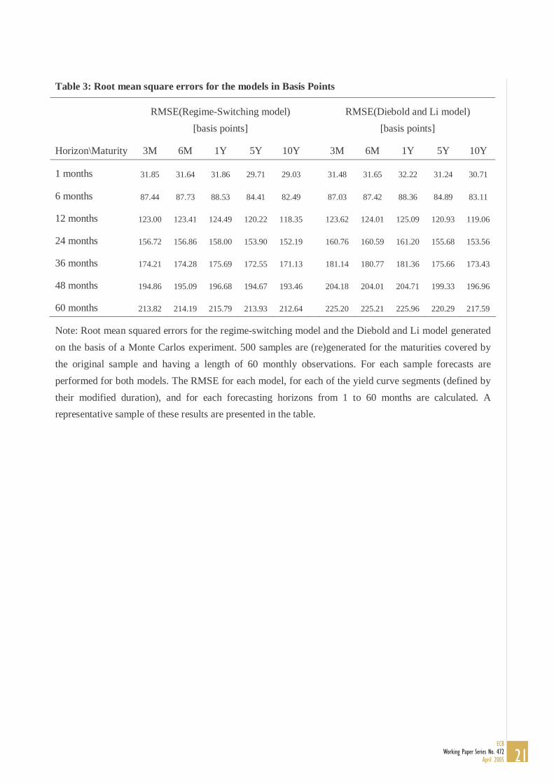
Table 3: Root mean square errors for the models in Basis Points

RMSE(Regime-Switching model)

[basis points]

RMSE(Diebold and Li model)

[basis points]

Horizon\Maturity 3M 6M 1Y 5Y 10Y 3M 6M 1Y 5Y 10Y

1 months 31.85 31.64 31.86 29.71 29.03 31.48 31.65 32.22 31.24 30.71

6 months 87.44 87.73 88.53 84.41 82.49 87.03 87.42 88.36 84.89 83.11

12 months 123.00 123.41 124.49 120.22 118.35 123.62 124.01 125.09 120.93 119.06

24 months 156.72 156.86 158.00 153.90 152.19 160.76 160.59 161.20 155.68 153.56

36 months 174.21 174.28 175.69 172.55 171.13 181.14 180.77 181.36 175.66 173.43

48 months 194.86 195.09 196.68 194.67 193.46 204.18 204.01 204.71 199.33 196.96

60 months 213.82 214.19 215.79 213.93 212.64 225.20 225.21 225.96 220.29 217.59

Note: Root mean squared errors for the regime-switching model and the Diebold and Li model generated

on the basis of a Monte Carlos experiment. 500 samples are (re)generated for the maturities covered by

the original sample and having a length of 60 monthly observations. For each sample forecasts are

performed for both models. The RMSE for each model, for each of the yield curve segments (defined by

their modified duration), and for each forecasting horizons from 1 to 60 months are calculated. A

representative sample of these results are presented in the table.

21ECB


Annex 2: Figures

Figure 1: Yield curve and macroeconomic data

0.00

2.00

4.00

6.00

8.00

10.00

12.00

14.00

16.00

18.00

Da t e

3M

6M

1Y

2Y

3Y

5Y

7Y

10Y

-6.00

-1.00

4.00

9.00

14.00

19.00

D ate

GDP

CPI

Note: The upper panel shows the time-series evolution of the data used in the study for the

observed maturity segments {3months, 6months, 1year, 2year, 3year, 5year, 7year, 10year}. The

lower panel shows the time-series evolution of the macro-economic variables i.e. GDP and CPI

growth.


Figure 2: Estimates yield curve factors, regime classifications and generic yield curves

-6.00

-1.00

4.00

9.00

14.00

19.00A

pr-5

3

Apr

-56

Apr

-59

Apr

-62

Apr

-65

Apr

-68

Apr

-71

Apr

-74

Apr

-77

Apr

-80

Apr

-83

Apr

-86

Apr

-89

Apr

-92

Apr

-95

Apr

-98

Apr

-01

Apr

-04

Date

Val

ue

Lev el

Slope

Curv ature

0.00

0.10

0.20

0.30

0.40

0.50

0.60

0.70

0.80

0.90

1.00

Date

Flat/Inverse

Steep

M ain

Note: The upper panel shows the evolution of the three estimated yield curve factors. Estimations are

performed on scaled data following [7], but results in the upper panel have been rescaled to enhance readability. The lower panel shows the obtained regime classifications and hence plots t tπ from [9].

23ECB


Figure 3: Forecast performance, comparing rmse of the Regime Switching model to the rmse of the

Diebold&Li model.

0 10 20 30 40 50 60-20

0

203 month rate

Month

Bas

is p

oint

s

0 10 20 30 40 50 60-20

0

206 month rate

Month

Bas

is p

oint

s

0 10 20 30 40 50 60-20

0

201 year rate

Month

Bas

is p

oint

s

0 10 20 30 40 50 60-20

0

202 year rate

MonthB

asis

poi

nts

0 10 20 30 40 50 60-20

0

203 year rate

Month

Bas

is p

oint

s

0 10 20 30 40 50 60-20

0

205 year rate

Month

Bas

is p

oint

s

0 10 20 30 40 50 60-20

0

207 year rate

Month

Bas

is p

oint

s

0 10 20 30 40 50 60-20

0

2010 year rate

Month

Bas

is p

oint

s

Note: Each sub-plot shows the difference between the root mean squared error (rmse) of the regime-

switching model and the rmse of the Diebold and Li method as well as 95% confidence limits, for the

different yield curve segments included in the original data sample. The full-lines depict RS DLrmse rmse− ,

so a negative number in the graph signifies better forecasting performance of the regime-switching model.

The dotted lines are 95% upper and lower confidence intervals calculated on the basis of Diebold and

Mariano (1995).


Figure 4: Distribution of GDP and inflation over the forecast horizon

-2

-1

0

1

2

3

4

0 10 20 30 40 50 60

Time [Months]

Main economic scenario Pessimistic economic scenario

0

1

2

3

4

5

0 10 20 30 40 50 60

Time [Months]

CPI

GDP CPI

GDP

Note: Two hypothetical macro economic scenarios are show for the evolution of GDP and CPI growth.

The forecasting horizon is 60 months and the scenarios represent a main economic evolution (in the left

most panel) and a pessimistic macro scenario (in the right most panel).

25ECB


Figure 5: Evolution of average state probabilities and yield curve

10 20 30 40 50 600

0.1

0.2

0.3

0.4

0.5

0.6

0.7

0.8

0.9

1

Time [Months]

Pro

bab

ility

10 20 30 40 50 600

0.1

0.2

0.3

0.4

0.5

0.6

0.7

0.8

0.9

1

Time [Months]

Pro

bab

ility


Steep

Normal

Inverse

Steep

Normal

Inverse

Horizon Horizon

Maturity Maturity

Yield Yield

Note: The left panel shows the evolution of the regime probabilities over the forecasting horizon and the

resulting projected yield curve surface, for a hypothetical main economic scenario. The right panel shows

the evolution of regime probabilities and the yield curve surface when the hypothetical macro scenarios is

based on a pessimistic economic scenario. The hypothetical evolutions correspond to the example

projections for GDP and CPI growth depicted in Figure 4.


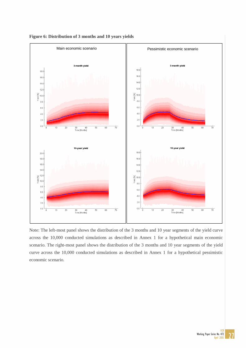
Figure 6: Distribution of 3 months and 10 years yields


Note: The left-most panel shows the distribution of the 3 months and 10 year segments of the yield curve

across the 10,000 conducted simulations as described in Annex 1 for a hypothetical main economic

scenario. The right-most panel shows the distribution of the 3 months and 10 year segments of the yield

curve across the 10,000 conducted simulations as described in Annex 1 for a hypothetical pessimistic

economic scenario.

27ECB



European Central Bank working paper series

For a complete list of Working Papers published by the ECB, please visit the ECB’s website(http://www.ecb.int)

425 “Geographic versus industry diversification: constraints matter” by P. Ehling and S. B. Ramos,January 2005.

426 “Security fungibility and the cost of capital: evidence from global bonds” by D. P. Millerand J. J. Puthenpurackal, January 2005.

427 “Interlinking securities settlement systems: a strategic commitment?” by K. Kauko, January 2005.

428 “Who benefits from IPO underpricing? Evidence form hybrid bookbuilding offerings”by V. Pons-Sanz, January 2005.

429 “Cross-border diversification in bank asset portfolios” by C. M. Buch, J. C. Driscolland C. Ostergaard, January 2005.

430 “Public policy and the creation of active venture capital markets” by M. Da Rin,G. Nicodano and A. Sembenelli, January 2005.

431 “Regulation of multinational banks: a theoretical inquiry” by G. Calzolari and G. Loranth, January 2005.

432 “Trading european sovereign bonds: the microstructure of the MTS trading platforms”by Y. C. Cheung, F. de Jong and B. Rindi, January 2005.

433 “Implementing the stability and growth pact: enforcement and procedural flexibility”by R. M. W. J. Beetsma and X. Debrun, January 2005.

434 “Interest rates and output in the long-run” by Y. Aksoy and M. A. León-Ledesma, January 2005.

435 “Reforming public expenditure in industrialised countries: are there trade-offs?”by L. Schuknecht and V. Tanzi, February 2005.

436 “Measuring market and inflation risk premia in France and in Germany”by L. Cappiello and S. Guéné, February 2005.

437 “What drives international bank flows? Politics, institutions and other determinants”by E. Papaioannou, February 2005.

438 “Quality of public finances and growth” by A. Afonso, W. Ebert, L. Schuknecht and M. Thöne,February 2005.

439 “A look at intraday frictions in the euro area overnight deposit market”by V. Brousseau and A. Manzanares, February 2005.

440 “Estimating and analysing currency options implied risk-neutral density functions for the largestnew EU member states” by O. Castrén, February 2005.

441 “The Phillips curve and long-term unemployment” by R. Llaudes, February 2005.

442 “Why do financial systems differ? History matters” by C. Monnet and E. Quintin, February 2005.

443 “Explaining cross-border large-value payment flows: evidence from TARGET and EURO1 data”by S. Rosati and S. Secola, February 2005.

444 “Keeping up with the Joneses, reference dependence, and equilibrium indeterminacy” by L. Straccaand Ali al-Nowaihi, February 2005.

29ECB


445 “Welfare implications of joining a common currency” by M. Ca’ Zorzi, R. A. De Santis and F. Zampolli,February 2005.

446 “Trade effects of the euro: evidence from sectoral data” by R. Baldwin, F. Skudelny and D. Taglioni,February 2005.

447 “Foreign exchange option and returns based correlation forecasts: evaluation and two applications”by O. Castrén and S. Mazzotta, February 2005.

448 “Price-setting behaviour in Belgium: what can be learned from an ad hoc survey?”by L. Aucremanne and M. Druant, March 2005.

449 “Consumer price behaviour in Italy: evidence from micro CPI data” by G. Veronese, S. Fabiani,A. Gattulli and R. Sabbatini, March 2005.

450 “Using mean reversion as a measure of persistence” by D. Dias and C. R. Marques, March 2005.

451 “Breaks in the mean of inflation: how they happen and what to do with them” by S. Corvoisierand B. Mojon, March 2005.

452 “Stocks, bonds, money markets and exchange rates: measuring international financial transmission” by M. Ehrmann, M. Fratzscher and R. Rigobon, March 2005.

453 “Does product market competition reduce inflation? Evidence from EU countries and sectors” by M. Przybyla and M. Roma, March 2005.

454 “European women: why do(n’t) they work?” by V. Genre, R. G. Salvador and A. Lamo, March 2005.

455 “Central bank transparency and private information in a dynamic macroeconomic model”by J. G. Pearlman, March 2005.

456 “The French block of the ESCB multi-country model” by F. Boissay and J.-P. Villetelle, March 2005.

457 “Transparency, disclosure and the federal reserve” by M. Ehrmann and M. Fratzscher, March 2005.

458 “Money demand and macroeconomic stability revisited” by A. Schabert and C. Stoltenberg, March 2005.

459 “Capital flows and the US ‘New Economy’: consumption smoothing and risk exposure”by M. Miller, O. Castrén and L. Zhang, March 2005.

460 “Part-time work in EU countries: labour market mobility, entry and exit” by H. Buddelmeyer, G. Mourreand M. Ward, March 2005.

461 “Do decreasing hazard functions for price changes make any sense?” by L. J. Álvarez, P. Burrieland I. Hernando, March 2005.

462 “Time-dependent versus state-dependent pricing: a panel data approach to the determinants of Belgianconsumer price changes” by L. Aucremanne and E. Dhyne, March 2005.

463 “Break in the mean and persistence of inflation: a sectoral analysis of French CPI” by L. Bilke, March 2005.

464 “The price-setting behavior of Austrian firms: some survey evidence” by C. Kwapil, J. Baumgartnerand J. Scharler, March 2005.

465 “Determinants and consequences of the unification of dual-class shares” by A. Pajuste, March 2005.

466 “Regulated and services’ prices and inflation persistence” by P. Lünnemann and T. Y. Mathä,April 2005.

467 “Socio-economic development and fiscal policy: lessons from the cohesion countries for the newmember states” by A. N. Mehrotra and T. A. Peltonen, April 2005.


468 “Endogeneities of optimum currency areas: what brings countries sharing a single currencycloser together?” by P. De Grauwe and F. P. Mongelli, April 2005.

469 “Money and prices in models of bounded rationality in high inflation economies”by A. Marcet and J. P. Nicolini, April 2005.

470 “Structural filters for monetary analysis: the inflationary movements of money in the euro area”by A. Bruggeman, G. Camba-Méndez, B. Fischer and J. Sousa, April 2005.

471 “Real wages and local unemployment in the euro area” by A. Sanz de Galdeano and J. Turunen,April 2005.

472 “Yield curve prediction for the strategic investor” by C. Bernadell, J. Coche and K. Nyholm,April 2005.

yield curve prediction for the strategic investor - european central

Documents