yield curve construction models - quantitative research
TRANSCRIPT

1 | P a g e M o d e l i n g t h e Y i e l d C u r v e J o n a t h a n K i n l a y & X u B a i
Yield Curve Construction Models – Tools & Techniques
Summary
Yield curve models are used to price a wide variety of interest rate-contingent claims. The existence of several
different competing methods of curve construction available and there is no single standard method for constructing
yield curves and alternate procedures are adopted in different business areas to suit local requirements and market
conditions. This fragmentation has often led to confusion amongst some users of the models as to their precise
functionality and uncertainty as to which is the most appropriate modeling technique. In addition, recent market
conditions, which inter-alia have seen elevated levels of LIBOR basis volatility, have served to heighten concerns
amongst some risk managers and other model users about the output of the models and the validity of the underlying
modeling methods.
The purpose of this review, which was carried out in conjunction with research analyst Xu Bai, now at Morgan
Stanley, was to gain a thorough understanding of current methodologies, to validate their theoretical frameworks and
implementation, identify any weaknesses in the current modeling methodologies, and to suggest improvements or
alternative approaches that may enhance the accuracy, generality and robustness of modeling procedures.
Model Description
In this section, we describe in detail the three methodologies used in the curve construction. We choose the curve
inputs as of 01/22/2008 as the typical set-up so that we have a concrete example based on which we can write the
documentation and do testing and analyses. As shown in the chart below, this typical set-up includes two cash
points, sixteen futures points and fifteen swap points. The basic requirement for a curve construction methodology is
to correctly price the input instruments. However the interpolation methods will differ as we shall see in the
following sections.
Table
1: Cash, Futures and Swap Data Grid
RAW METHODOLOGY
The RAW is the simplest among the four methodologies. The interpolation in RAW is basically log-linear, or linear
interpolation of logarithm of the discount factors, which results in piecewise linear forward rate curves. The
procedure to build up a curve using RAW can be decomposed into four steps: turn-adjustment, add-cash-points, add-
futures-points and add-swap-points.
Turn-adjustment
The year-end turn of the yield curve is defined as the sudden jump in yields during the change of the year. This
usually happens at the end of the calendar year, reflecting increased market activity related to year-end portfolio
adjustments and hedging activity. However the turn can be at other times of the year, for instance around common

2 | P a g e M o d e l i n g t h e Y i e l d C u r v e J o n a t h a n K i n l a y & X u B a i
financial year end dates such as the March-April period in the Japanese market. Currently methodology permits the
yield curve to have turns only in the futures sector. When there is a year turn(s), two discount curves are
constructed: one for turn discount factors and one for the discount factors calculated from the input instruments after
adjustments and the discount factor at any time is the multiplication of two.
The very first turn is a user input: the user can specify the turn start date, for example the last business day of the
year, the turn end date, usually the first business day of the following year and the turn spread. We use the
following notation:
T otalPeriod=number of days in the futures period that comprises the year turn
T urnPeriod=number of days in the turn period
InputT urnSpread=user defined turn spread in bps
AdjustedT urnSpread=turn spread adjusted after lowering the corresponding futures implied rate
Then the turn discount factor can be calculated as follows:
T urnPeriod T urnEndDate T urnStartDate
T otalPeriod FuturesEndDate FutureStartDate
AdjustedT urnSpread InputT urnSpread * T otalPeriod / (T otalPeriod T urnPeriod )
T urnDiscountFactor exp( AdjustedT urnSpread * T otalPer
3650000iod / )
To lower the futures implied rate accordingly, we have:
360FutDcf=futures daycount fraction=T otalPeriod /
FutDiscFactor=discount factor implied by the futures price before adustment
=1/ (1+FutRate*FutDcf)
FutRate=futures implied rate=1-(FuturesPrice+Convexity)/ 10000
AdjustedFutRate=(T urnDiscountFactor / FutDiscFactor-1)/ FutDcf
The reason for adjusting the turn spread and the futures implied rate is to ensure the equality of the integral of the
forward rates before and after the adjustments.
After the first turn inputted by user, the far turns are implied by the futures prices. For instance, there are a turn in
Dec09-Jan10 and another turn in Dec10-Jan11. The implied spread is calculated using three futures that are close to
the turn:
1 110000 2i i i
i
i-1
i+1
Im pledSpread * FutRate FutRate / FutRate
FutRate : rate implied by the futures that straddles the turn
FutRate : rate implied by the futures before
FutRate : rate implied by the futur
es after
From the formulae we can see that nothing a priori excludes a negative implied spread. Then the turn discount factor
and the adjusted futures implied rate can be calculated similarly as for the first turn:
T urnDiscountFactor=exp(-ImpliedSpread*T otalPeriod*T otalPeriod/ (T otalPeriod T urnPeriod)/ 3650000)
AdjustedFutRate=(T urnDiscountFactor / FutDiscFactor-1)/ FutDcf
For each turn point, the cumulative value of logarithm of turn discount factor is stored along with the corresponding
turn date.
Add-cash-points

3 | P a g e M o d e l i n g t h e Y i e l d C u r v e J o n a t h a n K i n l a y & X u B a i
Once the turn discount curve has been constructed, we can proceed to add discount factors to the regular discount
curve by starting with the cash instruments. The cash rates are simple rates with act/360 daycount convention. The
discount factors can be calculated from the cash rates as follows:
1 1DF / ( dcf * CashRate)
dcf=daycount fraction=(SpotDate-StartDate)/ 360
StartDate: curve start date
SpotDate: settlement date, usually 2 days from the start date
CashPointValue=log(DF)
CashPointDate=CashRateD
ate
So far we have added three points to the curve: DF(StartDate), DF(2D) and DF(3M). The very first point
DF(StartDate) is equal to one of course.
Add-futures-points
There are 16 futures in our example and therefore we have to add 16 discount factors to the curve. As the first
futures point (MAR08) is overlapped with the last cash point (3M), we have to replace the last cash point by the first
futures point. Therefore the date for the last cash point is not 3M anymore and is replaced by 03-19-08. The
corresponding curve point value is given by log-linear interpolation as follows:
360
1
dcf ( FutEndDate FutStartDate) /
LogDF log( dcf * FutRate)
LastCashPo intValue LastY iledCurvePo intValue LogDF * ( LastCashPo int Date FutStartDate)...
/ ( FutEndDate FutStartDate)
For other futures points, the following formulas are used:
360
1
dcf ( FutEndDate FutStartDate) /
LogDF log( dcf * FutRate)
FutPo intValue LastFutPo intValue LogDF
FutPo int Date FutEndDate
Add-swap-points
The discount factors on the swap dates are calculated using the traditional bootstrapping technique: given the
previous found discount factors and log-linear interpolation, one find the discount factor or precisely the increment
of logarithm of discount factor at the swap maturity date that makes equal the fixed leg and the floating leg of the
swap. The fixed leg is usually semi-annual with 30/360 day count convention while the floating leg is quarterly with
act/360 day count convention. Mathematically we have:
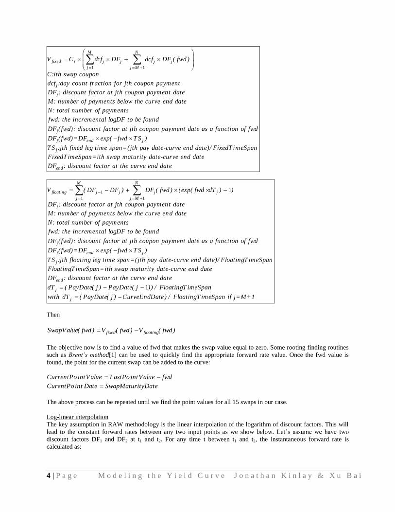
4 | P a g e M o d e l i n g t h e Y i e l d C u r v e J o n a t h a n K i n l a y & X u B a i
1 1
M N
fixed i j j j j
j j M
j
j
V C dcf DF dcf DF ( fwd )
C:ith swap coupon
dcf :day count fraction for jth coupon payment
DF : discount factor at jth coupon payment date
M: number of payments below the curve
j
j end j
j
end date
N: total number of payments
fwd: the incremental logDF to be found
DF (fwd): discount factor at jth coupon payment date as a function of fwd
DF (fwd)=DF exp( fwd T S )
T S :jth fixed leg time sp
end
an=(jth pay date-curve end date)/ FixedT imeSpan
FixedT imeSpan=ith swap maturity date-curve end date
DF : discount factor at the curve end date
1
1 1
1
M N
floating j j j j
j j M
j
V ( DF DF ) DF ( fwd ) (exp( fwd dT ) )
DF : discount factor at jth coupon payment date
M: number of payments below the curve end date
N: total number of payments
fwd: the incremental
j
j end j
j
logDF to be found
DF (fwd): discount factor at jth coupon payment date as a function of fwd
DF (fwd)=DF exp( fwd T S )
T S :jth floating leg time span=(jth pay date-curve end date)/ FloatingT imeSpan
Float
1
end
j
j
ingT imeSpan=ith swap maturity date-curve end date
DF : discount factor at the curve end date
dT ( PayDate( j ) PayDate( j )) / FloatingT imeSpan
with dT ( PayDate( j ) CurveEndDate) / FloatingT imeSpan if j=M+1
Then
fixed floatingSwapValue( fwd) V ( fwd) V ( fwd)
The objective now is to find a value of fwd that makes the swap value equal to zero. Some rooting finding routines
such as Brent’s method[1] can be used to quickly find the appropriate forward rate value. Once the fwd value is
found, the point for the current swap can be added to the curve:
CurrentPo intValue LastPo intValue fwd
CurentPo int Date SwapMaturityDate
The above process can be repeated until we find the point values for all 15 swaps in our case.
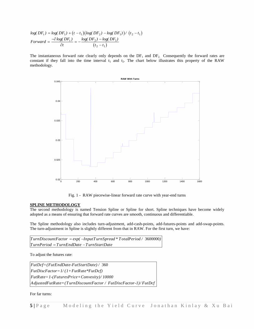
Log-linear interpolation
The key assumption in RAW methodology is the linear interpolation of the logarithm of discount factors. This will
lead to the constant forward rates between any two input points as we show below. Let’s assume we have two
discount factors DF1 and DF2 at t1 and t2. For any time t between t1 and t2, the instantaneous forward rate is
calculated as:
5 | P a g e M o d e l i n g t h e Y i e l d C u r v e J o n a t h a n K i n l a y & X u B a i
1 1 2 1 2 1
2 1
2 1
t
t
log( DF ) log( DF ) t t log( DF ) log( DF ) / t t
log( DF ) log( DF ) log( DF )Forward
t t t
The instantaneous forward rate clearly only depends on the DF1 and DF2. Consequently the forward rates are
constant if they fall into the time interval t1 and t2. The chart below illustrates this property of the RAW
methodology.
Fig. 1 - RAW piecewise-linear forward rate curve with year-end turns
SPLINE METHODOLOGY
The second methodology is named Tension Spline or Spline for short. Spline techniques have become widely
adopted as a means of ensuring that forward rate curves are smooth, continuous and differentiable.
The Spline methodology also includes turn-adjustment, add-cash-points, add-futures-points and add-swap-points.
The turn-adjustment in Spline is slightly different from that in RAW. For the first turn, we have:
3600000T urnDiscountFactor exp( InputT urnSpread * T otalPeriod / )
T urnPeriod T urnEndDate T urnStartDate
To adjust the futures rate:
360FutDcf=(FutEndDate-FutStartDate) /
FutDiscFactor=1/ (1+FutRate*FutDcf)
FutRate=1-(FuturesPrice+Convexity)/ 10000
AdjustedFutRate=(T urnDiscountFactor / FutDiscFactor-1)/ FutDcf
For far turns:
0 200 400 600 800 1000 1200 1400 16000.02
0.025
0.03
0.035
0.04
0.045RAW With Turns

6 | P a g e M o d e l i n g t h e Y i e l d C u r v e J o n a t h a n K i n l a y & X u B a i
1 110000 2i i i
i
i-1
i+1
Im pledSpread * FutRate FutRate / FutRate
FutRate : rate implied by the futures that straddles the turn
FutRate : rate implied by the futures before
FutRate : rate implied by the futur
es after
T urnDiscountFactor=exp(-ImpliedSpread*T otalPeriod/ 3600000)
AdjustedFutRate=(T urnDiscountFactor / FutDiscFactor-1)/ FutDcf
Add-cash-points1 and add-futures-points remain the same as in RAW. The big differences reside in the interpolation
method and the add-swap-points.
Tension-Spline Interpolator
The Spline methodology[2] was developed by FAST about ten years ago. Although the original documentation
describes that the instantaneous forward rate is modeled by a tension spline, an examination of the code revealed
that it is actually the (negative) logarithm of the discount factor (with some transformations) that is modeled.
A tension spline can have the following form on all intervals 1j jt , t :
0 1 2 3
1j j
f ( t ) a a t a exp( t ) a exp( t )
t t , t
is the tension parameter
When the sigma tends to zero, the tension spline degenerates into a regular cubic spline. On the other hand, when the
sigma increases, the tension spline asymptotically reduces to piecewise linear interpolation.
We describe briefly the curve modeling scheme using the tension spline. We have as inputs n discount factors iDF
and the associated dates iD and the following transformations are performed first:
1
1
1n
i i
i
i
i
T imeScaling=(t t ) / ( n )
T imeShift M T imeScaling
t D AsOfDate
n: number of points
t : ith discount factor maturity in days
D : ith discount factor date
DF :ith discount factor
AsOfDate: curve date
i i i
i i
i i i
Z ( log( DF )) / t
t ( t T imeShift ) / T imeScaling
Z Z t
With these transformations, the maturities of the discount factors will range from 1 to n and Z can be considered as
the negative logarithm of the discount factor on the new time axis. It is ultimately the Z and t that are modeled using
tension spline.
1 As we shall see soon we detected an inconsistency in overlapped cash-futures region which caused some excessive
swings for Spine interpolation.

7 | P a g e M o d e l i n g t h e Y i e l d C u r v e J o n a t h a n K i n l a y & X u B a i
For each transformed time interval 1j jt , t , a relative time scale is used again so that the time interval becomes
0 1t , t with 10 1 j jt =0 and t t t . Then the tension spline can be rewritten in the following form:
0 0 0 02 3
0 1
0
0
0
1
0 5
0 5
' '' '''
0 0
' '0 0
'' ''0
COSH SINH tZ( t ) Z Z t Z Z
t t , t
COSH . exp( t ) exp( t )
SINH . exp( t ) exp( t )
Z =Z(t ): value of Z at t
Z =Z (t ): first derivative of Z at t
Z =Z (t ): second derivative of Z a
0
0
''' '''0 0
t t
Z =Z (t ): third derivative of Z at t
We can easily verify that this form is equivalent to the form we defined earlier and the conditions are satisfied.
The key to have a smooth curve is not only make the function Z(t) go through the transformed input points, i.e.,
0 1Z(t ) and Z(t ) equal to the tabulated values at 0 1t and t for each interval, but also make the ' ''Z (t) and Z ( t )
equal at the joint points. Along with some boundary conditions, this is equivalent to solving a matrix equation whose
unique solution determines for each interval the values of ' '' '''0 0 0 0Z , Z , Z and Z which totally define the curve
through each time interval.
Add-swap-points
As the spline curve depends on neighboring points, one cannot use the usual bootstrapping technique to find the
discount factor that matches the input swap rate one after another. Instead a trial-and-error approach is used to
simultaneously find the discount factors that matched all input swap rates. Mathematically we have for the ith
swap:
1
1
1
Mifixed j j
j
j
j
Nifloating j j
j
j
V dcf DF
dcf :day count fraction for jth fixed coupon payment
DF : discount factor at jth coupon payment date
M: total number of fixed payments
V ( DF DF )
DF : discount fact
or at jth floating coupon payment date
N: total number of floating payments
Then the ith
swap rate is calculated as:
i i
i floating fixedSwapRate V / V
If we have K discount factor to be found in order to match K input swap rates (K=15 in our case), we can use a trial
vector 21 Kdf ,df ,...,df along with the discount factors we already found in cash and futures region to build up the
spline curve. Then we have to zero the following vector:
1 1 2 2 K K( SwapRate InputSwapRate ),( SwapRate InputSwapRate ),...,( SwapRate InputSwapRate )
8 | P a g e M o d e l i n g t h e Y i e l d C u r v e J o n a t h a n K i n l a y & X u B a i
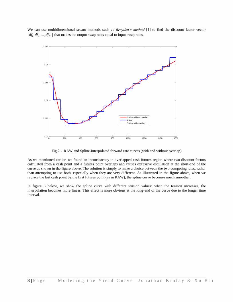
We can use multidimensional secant methods such as Broyden’s method [1] to find the discount factor vector
21 Kdf ,df ,...,df that makes the output swap rates equal to input swap rates.
Fig 2 - RAW and Spline-interpolated forward rate curves (with and without overlap)
As we mentioned earlier, we found an inconsistency in overlapped cash-futures region where two discount factors
calculated from a cash point and a futures point overlaps and causes excessive oscillation at the short-end of the
curve as shown in the figure above. The solution is simply to make a choice between the two competing rates, rather
than attempting to use both, especially when they are very different. As illustrated in the figure above, when we
replace the last cash point by the first futures point (as in RAW), the spline curve becomes much smoother.
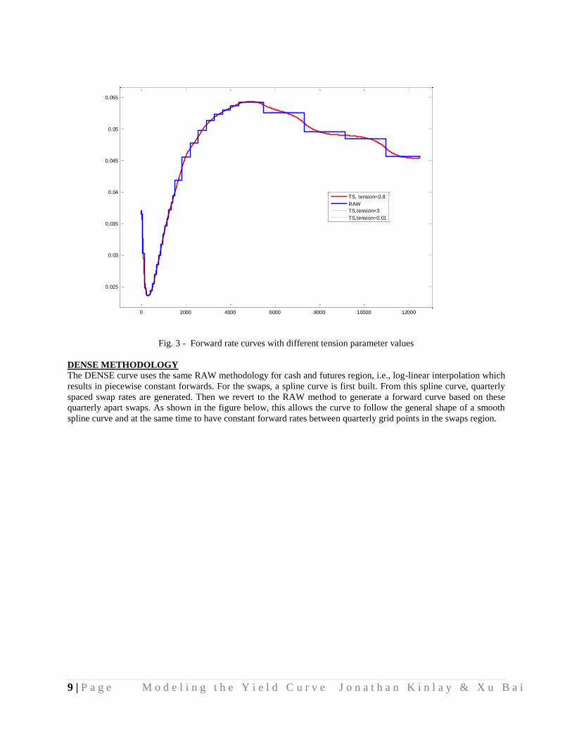
In figure 3 below, we show the spline curve with different tension values: when the tension increases, the
interpolation becomes more linear. This effect is more obvious at the long-end of the curve due to the longer time
interval.
0 200 400 600 800 1000 1200 1400 16000.02
0.025
0.03
0.035
0.04
0.045
Spline without overlap
RAW
Spline with overlap
9 | P a g e M o d e l i n g t h e Y i e l d C u r v e J o n a t h a n K i n l a y & X u B a i
Fig. 3 - Forward rate curves with different tension parameter values
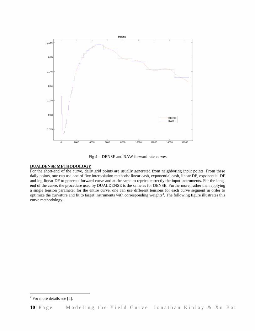
DENSE METHODOLOGY
The DENSE curve uses the same RAW methodology for cash and futures region, i.e., log-linear interpolation which
results in piecewise constant forwards. For the swaps, a spline curve is first built. From this spline curve, quarterly
spaced swap rates are generated. Then we revert to the RAW method to generate a forward curve based on these
quarterly apart swaps. As shown in the figure below, this allows the curve to follow the general shape of a smooth
spline curve and at the same time to have constant forward rates between quarterly grid points in the swaps region.
0 2000 4000 6000 8000 10000 12000
0.025
0.03
0.035
0.04
0.045
0.05
0.055
TS, tension=0.8
RAW
TS,tension=3
TS,tension=0.01
10 | P a g e M o d e l i n g t h e Y i e l d C u r v e J o n a t h a n K i n l a y & X u B a i
Fig 4 - DENSE and RAW forward rate curves
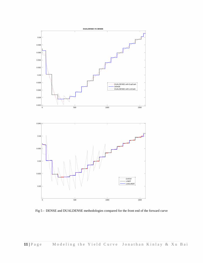
DUALDENSE METHODOLOGY
For the short-end of the curve, daily grid points are usually generated from neighboring input points. From these
daily points, one can use one of five interpolation methods: linear cash, exponential cash, linear DF, exponential DF
and log-linear DF to generate forward curve and at the same to reprice correctly the input instruments. For the long-
end of the curve, the procedure used by DUALDENSE is the same as for DENSE. Furthermore, rather than applying
a single tension parameter for the entire curve, one can use different tensions for each curve segment in order to
optimize the curvature and fit to target instruments with corresponding weights2. The following figure illustrates this
curve methodology.
2 For more details see [4].
0 2000 4000 6000 8000 10000 12000 14000 16000
0.025
0.03
0.035
0.04
0.045
0.05
0.055
DENSE
DENSE
RAW
11 | P a g e M o d e l i n g t h e Y i e l d C u r v e J o n a t h a n K i n l a y & X u B a i
Fig 5 - DENSE and DUALDENSE methodologies compared for the front end of the forward curve
0 500 1000 1500
0.022
0.024
0.026
0.028
0.03
0.032
0.034
0.036
0.038
0.04
DUALDENSE VS DENSE
DUALDENSE with ExpCash
DENSE
DUALDENSE with LinCash
0 500 1000 1500
0.02
0.025
0.03
0.035
0.04
0.045
EXPDF
LINDF
LOGLINDF
12 | P a g e M o d e l i n g t h e Y i e l d C u r v e J o n a t h a n K i n l a y & X u B a i
Extensions and Alternative Approaches
Tension / Smoothed Splines
The tension spline is the interpolation method employed by the SPLINE model and is the base of the DENSE and
DUALDENSE models.
Consider a standard cubic spline g(t) interpolating a set of data points (tj, gj), j = 1,…,M, where the tj are said to be
knot points. The spline function is piecewise linear in its second derivative:
Explicit equations for the interpolating spline can be recovered from the above by integrating the equation and
requiring the curve to pass through the given grid points, as well as having continuous first derivatives across knots.
To uniquely specify the cubic spline, derivative boundary conditions must be specified at t = t1 and t = tM. The so-
called natural spline has boundary conditions setting the second derivative to zero at these end points.
Cubic splines suffer from the defect that large values of the second derivative are hard to achieve, making tight turns
difficult, and exhibit non-local behavior in the sense that perturbations at one point in the curve will have secondary
effects in regions of the curve far from the point of disturbance. Tension splines seek to remedy this by applying a
tensile force at the end-points of the spline, formally:
For = 0, this reduces to the standard cubic spline form.
Let φ be a representation of the yield curve such that
And let
be the curve we have used as a representation of the discount curve.
Now let V = cP
Where
V = (V1, . . . , VN)T is a vector of observable securities prices,
C = {cij} is an N x M matrix of cash flows and
P = (P(t1), . . . , P(tM))T is a vector of discount factors
Then we aim to minimize the norm
g '' tt j 1 t
t j 1 t j
g '' j
t t j
t j 1 t j
g '' j 1, t t j , t j 1
g '' t 2 g tt j 1 t
t j 1 t j
g '' j2 g j
t t j
t j 1 t j
g '' j 12 g j 1 , t t j , t j 1
P t P t, t
t1 , . . . , tMT
J1
NV cP T W2 V cP
t1
tM'' t 2 2 ' t 2 t

13 | P a g e M o d e l i n g t h e Y i e l d C u r v e J o n a t h a n K i n l a y & X u B a i
Where W is a diagonal N x M matrix of weights which can be used to assign different importance to various of the
benchmark securities and and are positive constants relating the smoothness and tension of the spline curve.
The first of the two terms in the norm consists of the standard least-squares penalty term.
The second term, is a weighted smoothness term which penalizes high second order gradients of to
avoid kinks an discontinuities.
The optional final term, penalizes oscillations and excess convexity/concavity.
The norm is typically minimized using Gauss-Newton iteration.
DUALDENSE also allows for non-uniform tension in the spline, with local tension parameters j. In this case the
norm to be minimized is:
One problem not addressed by the current methodology is the choice of smoothing constant . Wahba (1990)
provides a technique, referred to as generalized cross validation (GCV), for estimating by non-linear least squares
minimization of an expression in the form:
Where H is a band-diagonal matrix determined by the knot points of a B-spline basis.
We return to this issue in the section on Basis Splines methodology.
J1
NV cP T W2 V cP
j 1
M 1
t1
t j 1'' t 2
j2 ' t 2 t
min P T P T H
t1
tM'' t 2
2
t1
tM' t 2
14 | P a g e M o d e l i n g t h e Y i e l d C u r v e J o n a t h a n K i n l a y & X u B a i
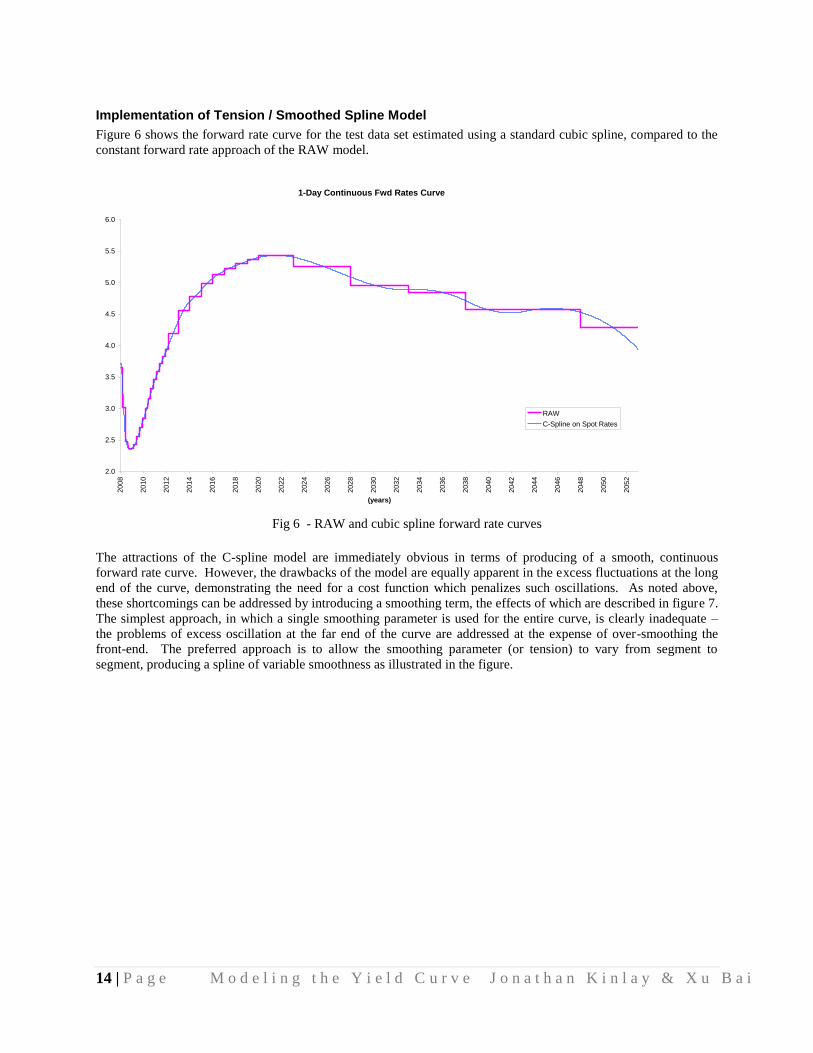
Implementation of Tension / Smoothed Spline Model
Figure 6 shows the forward rate curve for the test data set estimated using a standard cubic spline, compared to the
constant forward rate approach of the RAW model.
Fig 6 - RAW and cubic spline forward rate curves
The attractions of the C-spline model are immediately obvious in terms of producing of a smooth, continuous
forward rate curve. However, the drawbacks of the model are equally apparent in the excess fluctuations at the long
end of the curve, demonstrating the need for a cost function which penalizes such oscillations. As noted above,
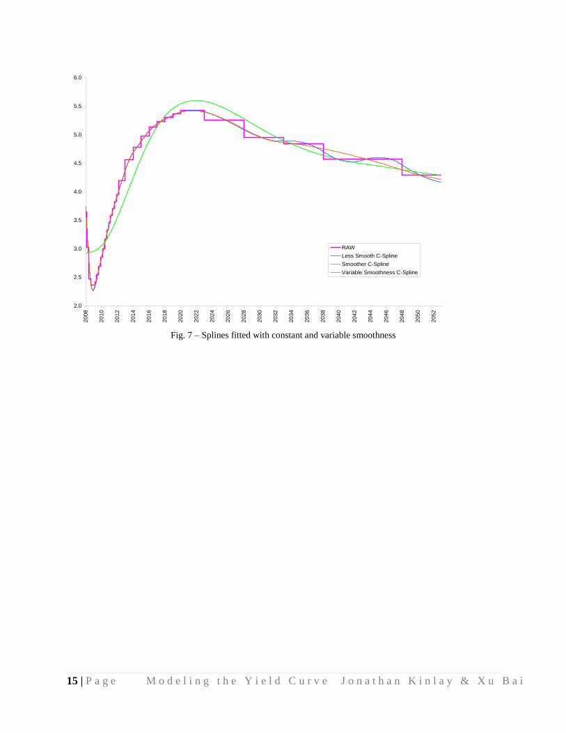
these shortcomings can be addressed by introducing a smoothing term, the effects of which are described in figure 7.
The simplest approach, in which a single smoothing parameter is used for the entire curve, is clearly inadequate –
the problems of excess oscillation at the far end of the curve are addressed at the expense of over-smoothing the
front-end. The preferred approach is to allow the smoothing parameter (or tension) to vary from segment to
segment, producing a spline of variable smoothness as illustrated in the figure.
1-Day Continuous Fwd Rates Curve
2.0
2.5
3.0
3.5
4.0
4.5
5.0
5.5
6.0
20
08
20
10
20
12
20
14
20
16
20
18
20
20
20
22
20
24
20
26
20
28
20
30
20
32
20
34
20
36
20
38
20
40
20
42
20
44
20
46
20
48
20
50
20
52
(years)
RAW
C-Spline on Spot Rates
15 | P a g e M o d e l i n g t h e Y i e l d C u r v e J o n a t h a n K i n l a y & X u B a i
Fig. 7 – Splines fitted with constant and variable smoothness
2.0
2.5
3.0
3.5
4.0
4.5
5.0
5.5
6.0
2008
2010
2012
2014
2016
2018
2020
2022
2024
2026
2028
2030
2032
2034
2036
2038
2040
2042
2044
2046
2048
2050
2052
RAW
Less Smooth C-Spline
Smoother C-Spline
Variable Smoothness C-Spline
16 | P a g e M o d e l i n g t h e Y i e l d C u r v e J o n a t h a n K i n l a y & X u B a i
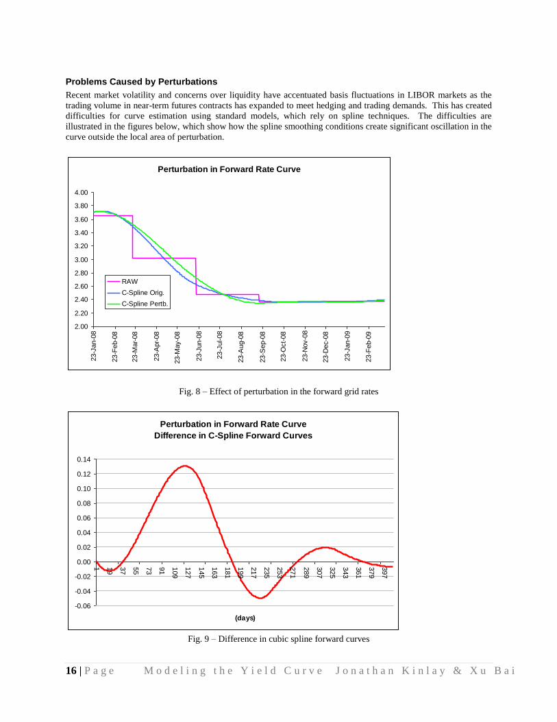
Problems Caused by Perturbations
Recent market volatility and concerns over liquidity have accentuated basis fluctuations in LIBOR markets as the
trading volume in near-term futures contracts has expanded to meet hedging and trading demands. This has created
difficulties for curve estimation using standard models, which rely on spline techniques. The difficulties are
illustrated in the figures below, which show how the spline smoothing conditions create significant oscillation in the
curve outside the local area of perturbation.
Fig. 8 – Effect of perturbation in the forward grid rates
Fig. 9 – Difference in cubic spline forward curves
Perturbation in Forward Rate Curve
2.00
2.20
2.40
2.60
2.80
3.00
3.20
3.40
3.60
3.80
4.00
23-J
an-0
8
23-F
eb-0
8
23-M
ar-
08
23-A
pr-
08
23-M
ay-0
8
23-J
un-0
8
23-J
ul-08
23-A
ug-0
8
23-S
ep-0
8
23-O
ct-
08
23-N
ov-0
8
23-D
ec-0
8
23-J
an-0
9
23-F
eb-0
9
RAW
C-Spline Orig.
C-Spline Pertb.
Perturbation in Forward Rate Curve
Difference in C-Spline Forward Curves
-0.06
-0.04
-0.02
0.00
0.02
0.04
0.06
0.08
0.10
0.12
0.141 19
37
55
73
91
109
127
145
163
181
199
217
235
253
271
289
307
325
343
361
379
397
(days)
17 | P a g e M o d e l i n g t h e Y i e l d C u r v e J o n a t h a n K i n l a y & X u B a i
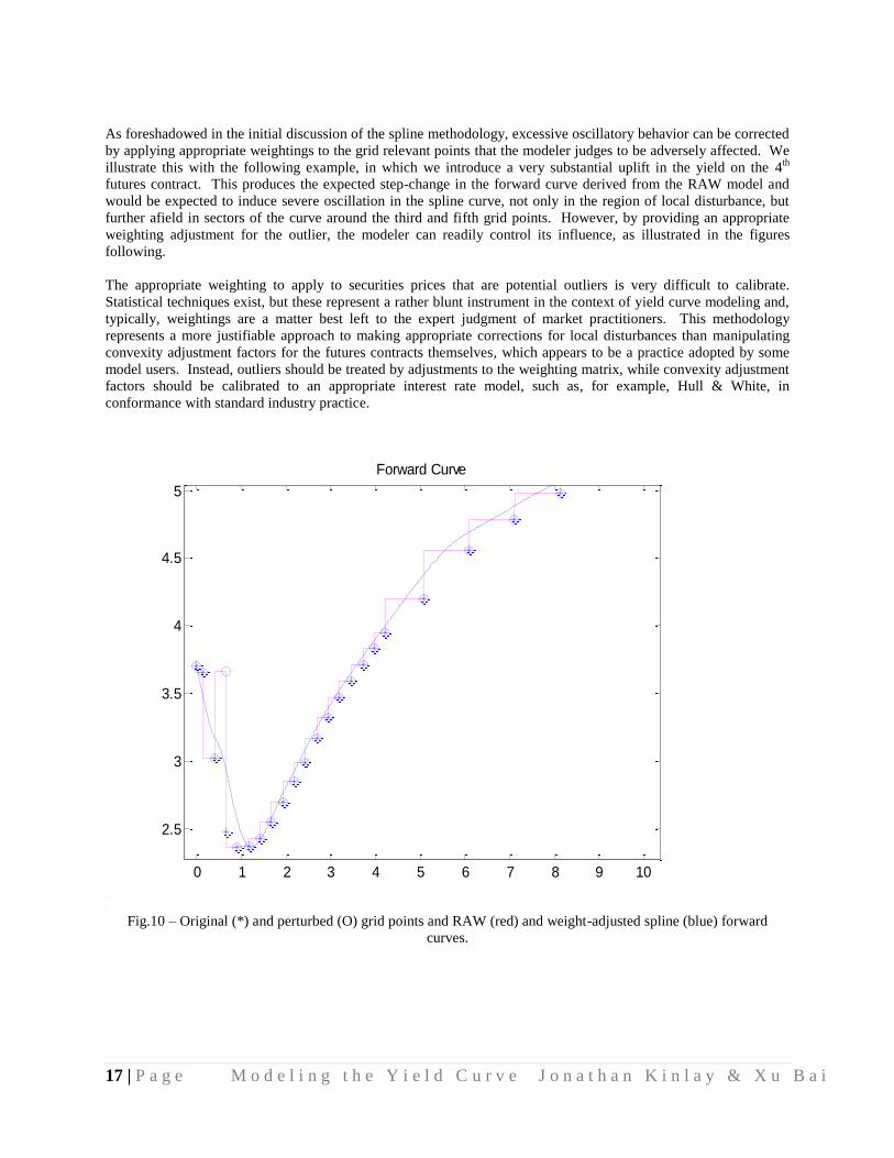
As foreshadowed in the initial discussion of the spline methodology, excessive oscillatory behavior can be corrected
by applying appropriate weightings to the grid relevant points that the modeler judges to be adversely affected. We
illustrate this with the following example, in which we introduce a very substantial uplift in the yield on the 4th
futures contract. This produces the expected step-change in the forward curve derived from the RAW model and
would be expected to induce severe oscillation in the spline curve, not only in the region of local disturbance, but
further afield in sectors of the curve around the third and fifth grid points. However, by providing an appropriate
weighting adjustment for the outlier, the modeler can readily control its influence, as illustrated in the figures
following.
The appropriate weighting to apply to securities prices that are potential outliers is very difficult to calibrate.
Statistical techniques exist, but these represent a rather blunt instrument in the context of yield curve modeling and,
typically, weightings are a matter best left to the expert judgment of market practitioners. This methodology
represents a more justifiable approach to making appropriate corrections for local disturbances than manipulating
convexity adjustment factors for the futures contracts themselves, which appears to be a practice adopted by some
model users. Instead, outliers should be treated by adjustments to the weighting matrix, while convexity adjustment
factors should be calibrated to an appropriate interest rate model, such as, for example, Hull & White, in
conformance with standard industry practice.
Fi Fig.10 – Original (*) and perturbed (O) grid points and RAW (red) and weight-adjusted spline (blue) forward
curves.
0 1 2 3 4 5 6 7 8 9 10
2.5
3
3.5
4
4.5
5
Forward Curve

18 | P a g e M o d e l i n g t h e Y i e l d C u r v e J o n a t h a n K i n l a y & X u B a i
Fig 11 – Original (*) and perturbed (O) spot curve grid points and RAW (red) and spline (blue) spot rate curves
Basis Spline Modelling
Under the B-spline scheme, a spline function f is defined as a linear combination of underlying spline functions
known as basis splines, each of which is positive on some interval defined by knot points. More formally,
Where Bik is the ith
order spline of order k, with knot points t(i), …, t(k), over which interval it is positive in value.
It is a piecewise polynomial of order k with breaks at the knot points t(i), …, t(k). These knots may coincide, and
the precise multiplicity governs the smoothness with which the two polynomial pieces join there.
For example, Fig 12 below shows a picture of a B-spline with knot sequence [0, 1.5, 2.3, 4, 5] which is of order 4,
together with the underlying polynomials that make up the spline.
-1 0 1 2 3 4 5 6 7 8
2.6
2.8
3
3.2
3.4
3.6
3.8
Spot Curve

19 | P a g e M o d e l i n g t h e Y i e l d C u r v e J o n a t h a n K i n l a y & X u B a i
Fig. 12 – a B-spline of order 4 and the cubic polynomials of which it is composed
We can use B-splines to represent the discount function, the spot rate curve, the forward rate curve, or some function
of these and later in this report we discuss some of the pros and cons of the alternative approaches. For now, we
focus on modeling the spot rate grid.
As before, we employ norm minimization to identify the B-spine form of the smoothest function that lies within a
specified tolerance of the specified spot rate grid (t(j), s(j), j = 1, . . ., M.
The penalty function contains both a distance metric
and a roughness measure
where denotes the mth
derivative of f and W is a N x M matrix of weights which can be used to assign
different importance to various of the grid inputs.
The spline f is determined as the unique minimizer of the expression
where is a smoothing parameter.
This methodology provides an automated procedure for estimating parameters that result in a curve which closely
fits the grid data with a smooth, continuous forward rate curve with a B-Spline function for which the number and
0 1 2 3 4 5-1
-0.5
0
0.5
1
1.5
2
20 | P a g e M o d e l i n g t h e Y i e l d C u r v e J o n a t h a n K i n l a y & X u B a i
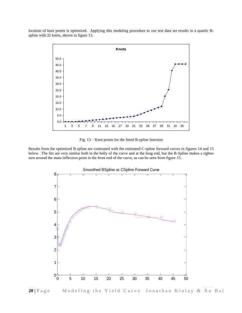
location of knot points is optimized. Applying this modeling procedure to our test data set results in a quartic B-
spline with 32 knots, shown in figure 13.
Fig. 13 – Knot points for the fitted B-spline function
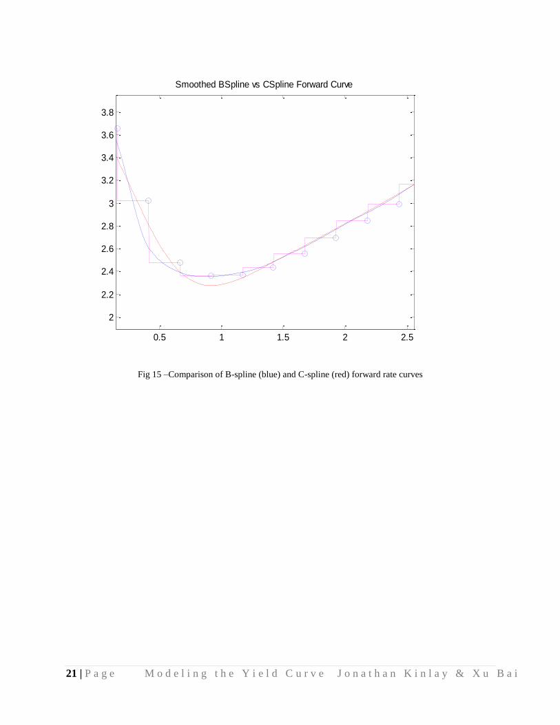
Results from the optimized B-spline are contrasted with the estimated C-spline forward curves in figures 14 and 15
below. The fits are very similar both in the belly of the curve and at the long end, but the B-Spline makes a tighter
turn around the main inflection point in the front end of the curve, as can be seen from figure 15.
Fig 14 – Comparison of B-spline (blue) and C-spline (red) forward rate curves
Knots
0.0
5.0
10.0
15.0
20.0
25.0
30.0
35.0
40.0
45.0
50.0
1 3 5 7 9 11 13 15 17 19 21 23 25 27 29 31 33 35
0 5 10 15 20 25 30 35 40 45 500
1
2
3
4
5
6
7
8Smoothed BSpline vs CSpline Forward Curve
21 | P a g e M o d e l i n g t h e Y i e l d C u r v e J o n a t h a n K i n l a y & X u B a i
Fig 15 –Comparison of B-spline (blue) and C-spline (red) forward rate curves
0.5 1 1.5 2 2.5
2
2.2
2.4
2.6
2.8
3
3.2
3.4
3.6
3.8
Smoothed BSpline vs CSpline Forward Curve

22 | P a g e M o d e l i n g t h e Y i e l d C u r v e J o n a t h a n K i n l a y & X u B a i
Perturbation and Smoothing of the B-Spline curve
As with the C-spline model, weights can be applied to the spot rates at the each grid point to reduce the impact of
outliers. Applying the same shock to the 4th
futures contract as before, and reducing the weighting of the 4th
grid
point relative to its near neighbors, results in a curve that smoothes out the effects of the outlier, as illustrated in the
figure 16.
Fig 16 –Comparison of original B-spline (blue) and smoothed B-spline (red) forward rate curves after perturbation
to the futures grid data
Procedures for Handling Outliers
Procedures for handling outliers have taken on additional importance given recent market turbulence, which has
produced unusually high levels of volatility in the LIBOR basis as investors seek to adjust position hedges and/or
favor safe-haven investments. The greatest effects are seen in the near-term Eurodollar futures contracts, and these
price “aberrations” are transmitted onwards through the strip as investors roll futures positions. To the extent that
analyst believes that, under conditions of market stress, certain individual futures prices are outliers with respect to
the true underlying forward rate curve, it makes sense to consider methods by which adjustments can be made to the
estimation methodology that will produce more reliable curve estimates.
Weighting
Making adjustments to the weight matrix, as described earlier in this report, is an appropriate and effective method
of handling outliers, but the procedure is somewhat arbitrary since it relies exclusively on the judgment of the
analyst. A more systematic approach that reflects current concerns about liquidity effects at the front of the futures
strip would be to derive weights based on (changes in) daily trading volumes and open interest. For example, to
take account of the forward-roll effect described above, weights for near-term futures contracts could be adjusted by
a factor representing a combination of the remaining term to maturity and changes in daily trading volume (relative
0.5 1 1.5 2 2.5
2.2
2.4
2.6
2.8
3
3.2
3.4
3.6
3.8
Perturbed Forward Curve

23 | P a g e M o d e l i n g t h e Y i e l d C u r v e J o n a t h a n K i n l a y & X u B a i
to open interest). Although we have not formulated a specific procedure in this analysis, it is likely that a feasible
result could be attained by a procedure of this kind.
FRAs
An alternative approach that deserves consideration would be to use FRA rates in the construction of the front of the
curve, supplementing and/or replacing some of the near-term futures contracts as the instruments of choice for
certain grid dates. This would serve as a consistency check for short term forward rates and help to identify outliers
in the futures strip. FRA’s have the added advantage of avoiding the need for convexity adjustments, which can
cause problems for an estimation procedure that is reliant on using futures prices exclusively. Liquidity in FRA
contracts is rapidly improving and this approach is probably viable as an adjunct to existing modelling procedures
for US$ and CAN$ curves. We understand that F.A.S.T. is currently developing new functionality to enable FRA
rates to be used in curve construction.
Which Grid Data to Fit?
One unanswered question is whether there are any relative advantages of fitting the curve to securities prices,
discount factors, spot rates, or to the forward rate grid.
To address this question we follow a procedure employed by Fisher, Nychka and Zervos (1994), using Monte Carlo
simulation to gauge the ability of the various estimation techniques to price securities accurately and to uncover the
true spot and forward rate curves. We begin by assuming a particular functional form for the forward term structure,
from which we generate “true” spot rates and zero coupon discount factors. Adding noise to these discount factors
we produce “observed” ZCB prices which include a Normal random term distributed with zero mean and
deterministic standard error . We then fit the term structure to each of these sets of generated data using various
functional forms and parameterizations, estimating an optimized B-spline curve using the generalized cross
validation (GCV) procedure described in the foregoing section of this report. This procedure is repeated in R
simulation runs.
We look at two sorts of criteria for goodness of fit, one relating to how well we uncover true zero coupon bond
prices and the other relating to how well we uncover spot and forward rate curves.
For bond prices we examine the mean absolute pricing error (MAPE):
Where the are the observed bond prices, and are the true bond prices at time ti.
For spot and forward rates we consider both the bias, which for a given maturity ti is defined as:
and the standard error, which for a given maturity ti is defined as:
Where ζ can refer to either the spot or forward rate.
MAPE1
Rnr 1
R
i 1
n
pr ti pr ti
B ti1
Rr 1
R
r ti r ti
S ti1
Rr 1
R
r ti1
Rr 1
R
r ti
2 1 2
pr ti pr ti

24 | P a g e M o d e l i n g t h e Y i e l d C u r v e J o n a t h a n K i n l a y & X u B a i
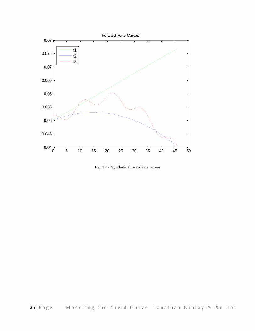
The function forms chosen for the forward rate curve for test purposes are as follows:
f1(t) = 0.05 + 0.000584t
f2(t) = 0.05 + 0.0004t - 0.0000133t2
f3(t) = 0.05 + 0.000266t + 0.000044t2 - 2.3×10⁻⁶t3 + 2.4×10⁻⁸ t4 + 0.002
Cos[0.566t]
In this test we assume that price volatility at time ti is function of the square root of time, i.e. where = 10
-5
Bias and standard errors are reported in basis points, while MAPE is reported in 1/10 basis point.
titi
25 | P a g e M o d e l i n g t h e Y i e l d C u r v e J o n a t h a n K i n l a y & X u B a i
0 5 10 15 20 25 30 35 40 45 500.04
0.045
0.05
0.055
0.06
0.065
0.07
0.075
0.08Forward Rate Curves
f1
f2
f3
Fig. 17 - Synthetic forward rate curves

26 | P a g e M o d e l i n g t h e Y i e l d C u r v e J o n a t h a n K i n l a y & X u B a i
Test Results Summary
Results from the testing process, using 100 runs of the Monte-Carlo simulation model, are shown in the charts and
tables following. In summary, in line with the results obtained by other researchers, we find that using forward rates
for curve estimation generally improves the ability to discover bond prices, as well as spot and forward rates, by a
significant margin. The pricing error in bond prices, as well as bias in estimated spot and forward rates, is typically
at least one order of magnitude smaller for curves fitted to forward rates, compared to other grid data, as can be seen
from Tables 2.1 – 2.3. Conversely, curves fitted to a grid of discount factors, the traditional approach originally
adopted by McCulloch, performs the worst of all three methods on most criteria, across all of the functional forms
considered here.
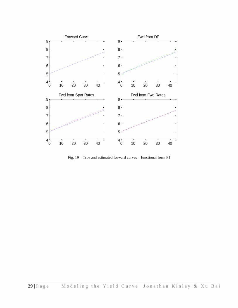
Turning to the detail of the results, for the linear functional form F1, all three techniques perform reasonably well in
fitting the spot and forward curves out to the 10-year horizon. Thereafter, however, both DF-fitted and spot rate-
fitted curves have an upward bias in the range of between 6 and 11 basis points in both spot and forward curves,
compared with a bias of less than 1/10 of a basis point for the forward rate-fitted curves (see charts in figure 18).
While the standard error of the spot rates is comparable amongst all three methods, the forward-rate fitted curve has
an average standard error in fitted forward rates that is significantly lower than for curves estimated by other
techniques.
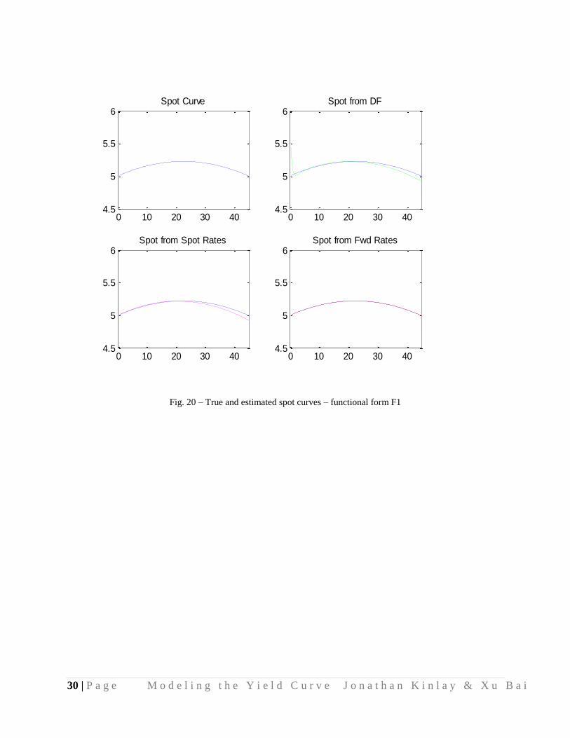
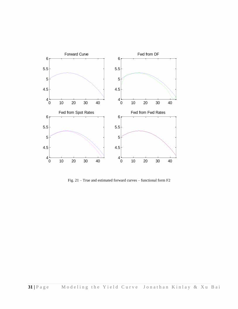
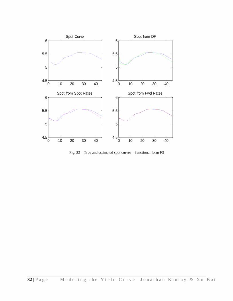
The same pattern of results holds for the second and third functional forms, as can be seen from figures 19 and 20
and the results in Tables 2.2. and 2.3. The error in the forward rate-fitted curve is an order of magnitude lower than
for other curves, on most goodness-of-fit criteria.
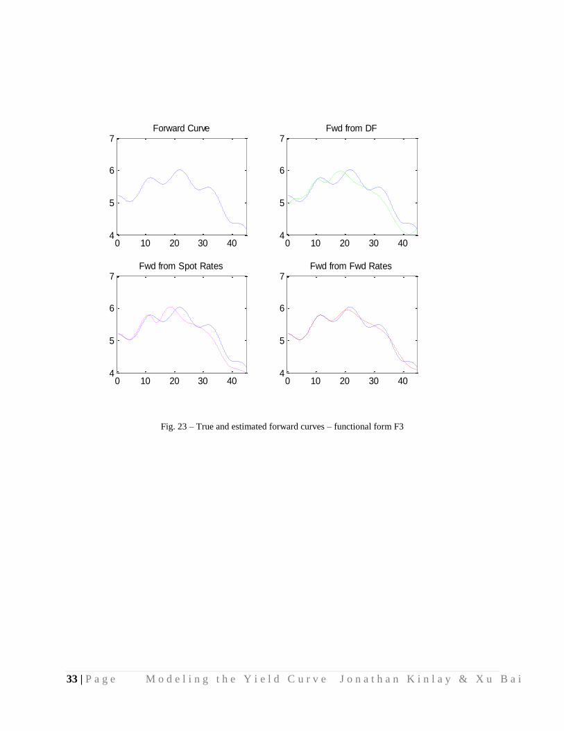
It is noteworthy that the B-spline GVC approach performs particularly well when applied to a forward rate grid
representing the most complex functional form F3. The curve fits the true forward curve closely at the front of the
curve where grid data is plentiful and then smoothes the curve in an appropriate manner (i.e. with increasing
linearity) from the 20-year maturity, when grid data becomes relatively scarce. Here, too, the average biases in
estimated spot and forward rates are an order of magnitude lower than for curves fitted to discount factors and spot
rates.

27 | P a g e M o d e l i n g t h e Y i e l d C u r v e J o n a t h a n K i n l a y & X u B a i
Goodness of Fit Test Results
Table 2.1 - Goodness of fit test results – functional form F1
Table 2.2 - Goodness of fit test results – functional form F2
Table 2.3 - Goodness of fit test results – functional form F3
Functional Form F1
ESTIMATION MAPE SPOT BIAS SPOT SE FWD BIAS FWD SE
DF 30.03 10.41 0.0013 11.39 0.0126
SPOT 29.71 6.27 0.0011 11.06 0.0136
FORWARD 0.42 0.04 0.0012 0.02 0.0095
Functional Form F2
ESTIMATION MAPE SPOT BIAS SPOT SE FWD BIAS FWD SE
DF 12.88 2.58 0.0012 -7.28 0.0078
SPOT 12.07 -1.65 0.0008 -7.08 0.0089
FORWARD 0.43 0.00 0.0011 -0.04 0.0078
Functional Form F3
ESTIMATION MAPE SPOT BIAS SPOT SE FWD BIAS FWD SE
DF 18.18 3.05 0.0021 -9.29 0.0088
SPOT 16.73 -0.68 0.0009 -8.94 0.0096
FORWARD 2.05 0.17 0.0012 -0.61 0.0079

28 | P a g e M o d e l i n g t h e Y i e l d C u r v e J o n a t h a n K i n l a y & X u B a i
Fig. 18 – True and estimated forward curves – functional form F1
0 10 20 30 404.5
5
5.5
6
6.5
7Spot Curve
0 10 20 30 404.5
5
5.5
6
6.5
7Spot from DF
0 10 20 30 404.5
5
5.5
6
6.5
7Spot from Spot Rates
0 10 20 30 404.5
5
5.5
6
6.5
7Spot from Fwd Rates
29 | P a g e M o d e l i n g t h e Y i e l d C u r v e J o n a t h a n K i n l a y & X u B a i
Fig. 19 – True and estimated forward curves – functional form F1
0 10 20 30 404
5
6
7
8
9Forward Curve
0 10 20 30 404
5
6
7
8
9Fwd from DF
0 10 20 30 404
5
6
7
8
9Fwd from Spot Rates
0 10 20 30 404
5
6
7
8
9Fwd from Fwd Rates
30 | P a g e M o d e l i n g t h e Y i e l d C u r v e J o n a t h a n K i n l a y & X u B a i
Fig. 20 – True and estimated spot curves – functional form F1
0 10 20 30 404.5
5
5.5
6Spot Curve
0 10 20 30 404.5
5
5.5
6Spot from DF
0 10 20 30 404.5
5
5.5
6Spot from Spot Rates
0 10 20 30 404.5
5
5.5
6Spot from Fwd Rates
31 | P a g e M o d e l i n g t h e Y i e l d C u r v e J o n a t h a n K i n l a y & X u B a i
Fig. 21 – True and estimated forward curves – functional form F2
0 10 20 30 404
4.5
5
5.5
6Forward Curve
0 10 20 30 404
4.5
5
5.5
6Fwd from DF
0 10 20 30 404
4.5
5
5.5
6Fwd from Spot Rates
0 10 20 30 404
4.5
5
5.5
6Fwd from Fwd Rates
32 | P a g e M o d e l i n g t h e Y i e l d C u r v e J o n a t h a n K i n l a y & X u B a i
Fig. 22 – True and estimated spot curves – functional form F3
0 10 20 30 404.5
5
5.5
6Spot Curve
0 10 20 30 404.5
5
5.5
6Spot from DF
0 10 20 30 404.5
5
5.5
6Spot from Spot Rates
0 10 20 30 404.5
5
5.5
6Spot from Fwd Rates
33 | P a g e M o d e l i n g t h e Y i e l d C u r v e J o n a t h a n K i n l a y & X u B a i
Fig. 23 – True and estimated forward curves – functional form F3
0 10 20 30 404
5
6
7Forward Curve
0 10 20 30 404
5
6
7Fwd from DF
0 10 20 30 404
5
6
7Fwd from Spot Rates
0 10 20 30 404
5
6
7Fwd from Fwd Rates

34 | P a g e M o d e l i n g t h e Y i e l d C u r v e J o n a t h a n K i n l a y & X u B a i
Recommendations
1. The SPLINE function should be changed to enable it to handle situations where there is inconsistency in
overlapped cash-futures grid rates.
2. Consideration should be given to developing a methodology to automatically adjust grid-point weights,
taking account of liquidity in the futures strip.
3. Analysts should be discouraged from using convexity adjustment factors to manipulate outlier futures
prices. Convexity adjustment factors should be derived from a suitable interest rate model, such as Hull-
White. Outliers should be handled by the weight-adjustment procedure.
4. Consideration should be given to incorporating FRA data in the construction of US$ and CAN$ curves.
5. Curves should be fitted to forward rate grid data rather than to spot rate or discount factor grid data.
6. The GCV B-Spline approach should be considered for implementation in a future release.

35 | P a g e M o d e l i n g t h e Y i e l d C u r v e J o n a t h a n K i n l a y & X u B a i
Acknowledgements
References
[1] Press, W. H., Flannery, B. P., Teukolsky, S. A., and Vettening, W. T., “Numerical Recipes in C++”, Cambridge
University Press, 2002.
[2] Sankar, L., “OFUTS – An Alternative Yield Curve Interpolator”, F.A.S.T. research documentation, Bear Stearns,
June 1997.
[3] Ezra Nahum, “Changes to Yield Curve Construction, Linear Stripping of Short End of the curve”, F.A.S.T.
research documentation, Bear Stearns, July 2004.
[4] “Dual Dense Yield Curve Methodology”, F.A.S.T. research documentation, Bear Stearns.
[5] Adams, K.J., and Van Deventer, D.R., “Fitting Yield Curves and Forward Rate Curves with Maximum
Smoothness”, Journal of Fixed Income, June (1994): 52-62
[6] Andersen, L., “Discount Curve Construction with Tension Splines”, Banc of America Securities (2005)
[7] De Boor, C., “A Practical Guide to Splines”, Springer-Verlag, (1978)
[8] Fisher, M., Nychka, D., and Zervos, D., “Fitting the Term Structure of Interest rates with Smoothing Splines”,
(1994)
[9] McCulloch, J.H., “Measuring the Term Structure of Interest Rates”, Journal of Business, 44 (1971): 19-31
[10] Wahba, G., “Spline Models for Observational Data”, SIAM; Philadelphia (1990)