yesterday's bad times are today's good old times: … · yesterday’s bad times are...
TRANSCRIPT

Finance and Economics Discussion Series Divisions of Research & Statistics and Monetary Affairs
Federal Reserve Board, Washington, D.C.
Yesterday’s Bad Times are Today’s Good Old Times: Retail Price Changes in the 1890s were Smaller, Less Frequent,
and More Permanent
Alan Kackmeister 2005-18
NOTE: Staff working papers in the Finance and Economics Discussion Series (FEDS) are preliminary materials circulated to stimulate discussion and critical comment. The analysis and conclusions set forth are those of the authors and do not indicate concurrence by other members of the research staff or the Board of Governors. References in publications to the Finance and Economics Discussion Series (other than acknowledgement) should be cleared with the author(s) to protect the tentative character of these papers.

Yesterday’s Bad Times are Today’s Good Old Times: Retail Price Changes in the 1890s were Smaller, Less Frequent, and More Permanent
This paper compares nominal price rigidity in retail stores during two 28-month periods: 1889-1891 and 1997-1999. The 1889-1891 microdata price quotes show: 1. a lower frequency of price changes; 2. a smaller average magnitude of price changes; 3. fewer “small” price changes; and, 4. fewer temporary price reductions. These differences are consistent with the 1889-1891 period having a higher cost of changing prices resulting in less adjustment to transitory price shocks. Changes in the retailing environment that may have led to a higher cost of changing prices in 1889-1891 are discussed.
Alan Kackmeister
Federal Reserve Board of Governors 20th St. and C St. NW Washington DC 20551
January 31, 2005
I would like to thank George Akerlof for encouragement, guidance, and countless suggestions. I would also like to thank Christina Romer, Barry Eichengreen, Catherine Wolfram, Peter Klenow, Chris Hanes, Bill Wascher, Paul Ruud, Jeff Frank, Steve Schutt, and many graduate students during my time at UC Berkeley for comments and suggestions. The views presented are solely those of the author and do not necessarily represent those of the Federal Reserve Board or its staff.

2
In the good old times in which the economists of the preceding generation lived, and from which they drew their economic illustrations and ideas, [price] changes seldom occurred, and when they did take place were very limited in extent, and came so slowly into effect as to attract no attention. All common articles of consumption had fixed prices which often did not change for a lifetime, and if any dealer had attempted to charge more than custom demanded, it would have attracted the attention and aroused the indignation of the whole community. These conditions have been so altered that to-day a merchant must consult his paper each day before he can know where to purchase a stock at the best advantage. The consumer also must be on his guard or he will pay too much for his sugar or flour. Dress goods and clothing, even at retail, fluctuate so rapidly in value that a study of advertisements is essential to a careful purchaser.
Simon N. Patten Professor of Political Economy Wharton School of Finance and Economy “The Stability of Prices” Publications of the American Economic Association January 1889
With a growing collection of microdata studies finding infrequent price changes, a next
step is to ask whether price changes today are more frequent or less frequent in the present than
in the past.1 The answer to this question may help explain differences in economic performance
across time. For example, if price movements reflect market forces then declining nominal price
rigidity–the time between price changes–may lead to improved resource allocation and higher
productivity, and may have important implications for business cycles and the transmission of
monetary policy.
As is related in the opening quote, over one-hundred years ago Simon Patten suggested
price changes were much more frequent by 1889 than they were “in the good old times”.
Unfortunately, Patten did not include quantitative support for his assertion, and little time—
series data exists before 1889 to verify his claim. However, even at the end of Patten’s period
the long life of retail prices is anecdotally supported by Levy and Young’s (2004) finding that
the retail price of a 6.5 ounce Coke remained unchanged for the 73 years from 1886 to 1959.
More recent studies using data from the 1950s through the 1980s, such as Cecchetti
(1986) (magazine prices), Carlton (1986) (wholesale industrial goods prices), and Kashyap
(1995) (apparel and outdoor goods prices from catalogs), find a shorter time between price
changes–on the order of one year. Even more recently, studies using retail price data from the
1 Among the studies looking at the frequency of price changes for the United States are: Carlton (1986), Cecchetti (1986), Kashyap (1995), Levy, et al. (1997), Bils and Klenow (2004).

3
1990s suggest the time between price changes may have decreased to around a few months.2
However, these studies differ so substantially in coverage and sources that the apparent decline
in price rigidity may be simply the result of different studies using different goods.
This leads to the central question of this paper: Has price rigidity declined over time?
Specifically, from the today’s perspective does 1889, Professor Patten’s age of rapidly fluctuating
prices, look like the “good old times” of highly rigid prices? To answer this question, goods
from 1889-1891 are compared with similar goods from 1997-1999. For each of these two periods,
broadly similar data sets are constructed covering retail price microdata over 28-months in 4
cities and up to 48 different product groups, including foods, household goods and clothing.
Over forty thousand first-differenced observations are available in each of the two periods. As
compared to 1997-1999, the data for 1889-1891 show:
(1) A lower frequency of retail price changes
(2) A smaller average magnitude of price changes
(3) Fewer “small” price changes, and
(4) Fewer temporary price reductions
Some changes in the retail environment that might explain these findings are discussed
in the last section. Most of the differences between the 1889-1891 and 1997-1999 data are
consistent with a higher cost of changing prices in 1889-1891 coupled with a high occurrence of
temporary price shocks.
Prior Microdata Studies and Wholesale vs. Retail prices
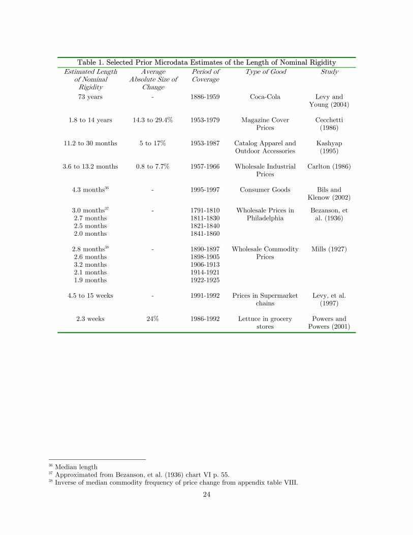
Numerous prior studies, dating back at least to Mills (1927), have examined the
frequency and size of price changes. A summary of results from some of these earlier studies is
presented in Table 1. The estimated time between price changes varies widely, ranging from
just over two weeks to nearly three-quarters of a century, while the absolute size of price
changes extends from less than one percent to nearly thirty percent.3
The huge differences in products across the studies in table 1 make drawing conclusions
about changes in the frequency or size of prices changes across time problematic. However, as
noted previously, there appears to be less nominal price rigidity in the more recent studies of
Bils and Klenow, and Levy, et al. than in the earlier studies of Cecchetti, Kashyap and Carlton.
2 Bils and Klenow (2004), Levy, et al (1997). 3 In all studies, observations where the price is unchanged are dropped from the calculation of the size of price changes.

4
Unlike the other studies listed in table 1, Bezanson, et al. (1936) and Mills (1927)
examine prices in more than a single time period, and these studies both also generally show a
downward drift in the frequency of price changes within the periods they cover. However, both
studies used wholesale rather than retail prices.
Wholesale prices suffer from three problems when attempting to ascertain the length of
nominal price rigidity. First, collected list prices might not reflect actual transaction prices
because wholesale products are often negotiated on a customer-by-customer basis.4 Second, the
effective good received by the purchaser might change over time as varying delivery lags and
other non-price means of allocation are common with wholesale goods.5 These two problems can
result in a constant price being observed when a price change should be recorded, which will
lead to an upward bias in the measurement of the length of nominal rigidity.
A third problem with wholesale prices is that wholesale prices are not unique. A single
unit may be sold many times before retail. For example, during the earlier period in this paper
at least three prices before retail were common: the price received by producers (or farmers); the
price received by large wholesalers; and the price received by jobbers, the small scale wholesalers
who bought from the large wholesalers and sold directly to the retail stores. Each of these
prices may have different characteristics.6 The inclusion of large wholesale auction market
prices, which are likely to exhibit little nominal rigidity, along with jobber prices may be the
reason that price changes appear to occur much more frequently in the studies of Mills and
Bezanson, et al.
Retail prices avoid most difficulties of wholesale prices. In retail markets price
negotiation seldom occurs, customers usually receive their goods immediately, and a single unit
of a product is sold at retail only once. These differences make retail prices preferable to
wholesale prices in determining price rigidity.
Retail prices, however, do have some problems. Temporary stock-outs can lead to
missing observations. Also, minor product specification changes may lead to the changed good
being classified as a new item, and can thereby hide a price change.7 Further, retail prices tend
to be heterogeneous with respect to brand and packaging sizes. The different brands and
4 Stigler and Kindahl (1973). 5 Carlton (1983, 1986), Morgenstern (1931), Dimand (2000), and Backman (1940 p. 485). Koelln and Rush (1993) in their critique of Cecchetti (1986) note a similar concept can apply to retail goods, for example when the number of pages in a magazine is reduced. 6 Backman (1940 p. 487) discusses market structure and price rigidity. 7 An example of this type of a minor product change occurred in 2001 when Kleenex reduced the number of tissues in a box from a 250 to a 230 but kept the same price. (Consumer Reports (2001)) Tissues are not included in any of the product groupings, and it is not known if minor specification changes hid price changes in any of the actual goods sampled.

5
package sizes may have different characteristics with respect to nominal price rigidity, and the
heterogeneity may itself lead to greater price rigidity as firms may have more market power.
The extent of these problems among the product sampled here is unknown, but minor product
specification changes and product heterogeneity–which lead to longer estimates of nominal
price rigidity–are probably more common in the 1997-1999 data sample, suggesting that
adjusting for them would strengthen the results found later in the paper.
An Overview of the Time Periods and Data
This study focuses on pricing across time, and therefore it is necessary to control for
factors that are not necessarily related to long-run changes across time but might cause different
pricing patterns between the two samples. Chief among these are different macroeconomic
conditions and data sampling methods in the two periods. The choice of data has minimized
these two potential problems. The macroeconomic conditions in 1889-1891 and 1997-1999, while
not identical, are similar enough that they are unlikely to cause major differences in the
microdata. For example, neither period includes a wartime economy, a sustained recession, or a
severe crash in the financial markets. (See table 2.) Nor were price controls or price supports
important during these periods. Also, both periods have similar inflation rates that are among
the lowest inflation episodes in the past one hundred and fifty years.8 The similarity in inflation
rates is extremely important when comparing the frequency of price changes across time because
aggregate inflation is one of the main causes of price changes. In a literature review Taylor
(1999) states:
The frequency of wage and price changes depends on the average rate of inflation... [P]rices at small businesses, industrial prices, and even the prices of products like magazines are adjusted more quickly when the rate of inflation is higher. This dependency of price and wage setting on events in the economy is one of the more robust empirical findings in the studies reviewed here. (p. 1021)
Further, the retail price microdata are surprisingly consistent on methodological
grounds. Both data sets are actual price quotes of retail establishments sampled by the Bureau
of Labor Statistics at a given point in each month. In both sets the prices quoted should closely
reflect transaction prices.9
8 Reliable estimates of aggregate consumer price inflation are not available for the 1889-1891 period, therefore table 2 shows wholesale price inflation. 9 There are a few relatively minor differences in methodology which are not expected to cause a problem, such as collecting the prices every month, which is the current practice, versus collecting the prices for the entire 28-month period from the merchant’s transaction records at the end of the period, which was the

6
However, methodologically-consistent time series of retail price microdata are not readily
available, and this has hampered the inclusion of additional time periods. Over the past 110
years, a handful of different institutions have created retail price indexes for the United States.
Most of the microdata used in creating these indexes has been lost or destroyed. To my
knowledge, there exist only four multi-good datasets of monthly time-series retail price
microdata for the United States, each covering only a very limited number of goods and years.
This study relies on the two broadest and most comparable sources of U.S. retail price
microdata: the 1892 Aldrich Report [Aldrich (1892)], an exhaustive study conducted by the
then-recently-formed Bureau of Labor Statistics covering, among other things, retail prices in
1889-1891, and the available microdata underlying the Bureau of Labor Statistics’ Consumer
Price Index, for which I have obtained a selection covering 1997-1999.10
The 1997-1999 dataset was specifically constructed to conform as closely as possible to
the available data from the 1889-1891 period. Starting and ending dates were chosen to match
the length and seasonality of the earlier data. Both datasets start in June and end in
September 27 months later. Products were chosen to maximize the number of comparable
product groups common to both samples. Localities were chosen to maximize the number of
localities with monthly price quotes in both samples.
Twenty-seven food products, seven clothing products, and fourteen household and
hardware products, for a total of forty-eight products, are common to both the Aldrich report
and current BLS CPI sample. Table 3 lists these 48 products. There also are four geographic
locations surveyed monthly in both samples: New York, Chicago, Los Angeles, and Newark.
Even within relatively disaggregated locations and products, substantial differences
among the sampled items is present within a group. For example, stores in high and low rent
areas might exist within a single location group, while only broadly related products might exist
within a single product group.11 Also, various sizes and brands of the same product might exist
within a single product group.12 For the purposes of this paper, it is assumed that all goods
within a given product or location group have similar price adjustment characteristics.
Basic statistics for the two datasets, shown in table 4, point out two important features
of the data. First, food prices, which tend to be volatile, comprise a larger share of the 1997-
practice for the 1889-1891 data. Methodology is described more fully in the data appendix and Appendix Table A3. 10 Microdata underlying the U.S. CPI currently exists only back to the late 1980s. All four potential sources of U.S. retail price microdata are described in the data appendix. 11 For example, onions, cabbages, and turnips all are part of the fresh vegetables product group. 12 This variation in sizes and brands makes price level dispersion for a single product impossible to calculate.
7
1999 data. This compositional difference will bias a simple average towards finding more
frequent price changes in 1997-1999. Second, both periods display a low unweighted average of
first-differenced log prices, and only slightly more upward price changes than downward price
changes. This reinforces the belief that inflation does not importantly influence the results.
How the 1890s differed from the 1990s
A lower frequency of price changes Nominal price rigidity in this paper is measured by the frequency of price changes (which
is the share of first-differenced observations where the price in time t does not equal the price in
time t-1).13 A higher frequency of price changes represents less nominal price rigidity. Using
the frequency of price changes, rather than average (or median) length of time between prices
changes, allows the inclusion of observations for which the beginning and/or ending of the spell
are missing from the dataset.
The lower overall frequency of price changes in the 1889-1891 sample is apparent from
the first two lines of table 4. The number of price changes in the 1889-1891 data is one-fifth of
that in the 1997-1999 data despite a similar number of first-differenced observations.
To check that the lower frequency of price changes in the 1889-1891 sample is not simply
a result of the difference in the share of food goods, or other differences in products, locations, or
seasonality between the two datasets, each observed price first-difference is classified into a cell
based on the location, product, and month. Then, the share of prices changing in a given cell in
the 19th century sample is compared with the corresponding cell in the 20th century sample.14
Dropping cells with less than 5 observations in each period leaves 1290 cells containing more
than 15,000 observations in each period for comparison.
This cells-based approach also suggests that prices changes were less frequent in the
earlier period. 909 of the 1290 cells, or 70%, have a lower frequency of price changes in 1889-
1891 than in 1997-1999. By comparison, only 254 cells, or 20%, show a higher frequency of
13 As observations are monthly, the inverse of the frequency of price changes is a slightly-upward-biased measure of the expected time between price changes. 14 To avoid multiple counting the months are numbered sequentially. For example, cells from the first month of the 1889-1891 sample, June 1889, are only compared with cells from the first month of the 1997-1999 sample, June 1997. Cells from July 1889 are compared to cells from July 1997, etc. The use of cells based on location, products, and months is conceptually similar to the approach currently used to create the lowest level indices in the CPI.

8
price changes in the earlier period. The remaining 127 cells, or 10%, show the same frequency
in each period.15
Differentiating observations only by location, by product, or by month, rather than all
three attributes, gives a more readily accessible view of the data. This view of the data is
shown in the three panels of figure 1.
In 43 of the 48 product groups the frequency of price changes was lower in 1889-1891
than in 1997-1999. These product groups are shown in the top panel of figure 1.
The lower frequency of price changes in 1889-1891 is much more pronounced for non-
food goods than for the food goods–a result of the extreme rigidity displayed by non-food goods
in the 1889-1891 sample. The twenty-one non-food product groups in the 1889-1891 sample
collectively contain 20,347 observations, but only 135 price changes. This amounts to an
average of one price change every 12-1/2 years!
A handful of food goods also displayed substantial nominal price rigidity in the 1889-
1891 sample. In the seven food product groups of coffee, tea, milk, beer, cornmeal, bread, and
salt and seasonings, collectively consisting of over 7,000 observations, only 38 price changes are
observed–an average of one price change every 15 years.
The few goods that had a fairly high frequency of price changes in the 1889-1891
period– eggs, sugar, butter, potatoes, and tomatoes–are staple goods, which might have been
used as loss leaders to bring in customers. Another possible cause of the high frequency of price
changes for eggs and butter in 1889-1891 is the presence of a strong seasonal cycle in prices of
these two products. This seasonality has since declined as the result of cheaper refrigeration.16
Pooling observations for a given location or month also shows a lower frequency of price
changes in the earlier period. The frequency of price changes rose in each location between the
two periods, though there is substantial variation in the frequency of price changes across the
different locations. (Figure 1B.) Also, every month in the 1997-1999 sample has a higher
frequency of price changes than the corresponding month in the 1889-1891 sample, and there is
no strong seasonality in the frequency of price changes in either period. (Figure 1C.)
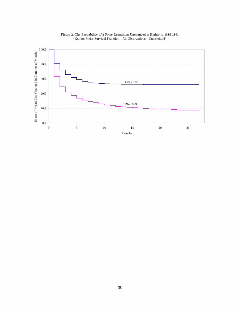
Pooling all observations and examining the Kaplan-Meier survival function shows just
how rigid prices were in the 1889-1891 data. (Figure 2.) The Kaplan-Meier survival function
gives the probability of a price remaining unchanged for a given length of time.17 In 1889-1891
15 This usually means that no price change was observed in either cell. 16 Goodwin, Grennes, and Craig (2002) show refrigeration had a strong effect on dampening the swings in butter prices. 17 The Kaplan-Meier methodology does not depend on a functional form. At each point in time the marginal probability of a price remaining unchanged between months t and t+1 is the share of prices with

9
the probability that a spell of nominal rigidity would extend at least 28 months was greater
than 50 percent. By comparison, the likelihood that spell of nominal rigidity would last at least
28 months in 1997-1999 was less than 20 percent. Moreover, for every length of time, the share
of price quotes remaining unchanged is higher in 1889-1891 than in 1997-1999 and the 95
percent confidence intervals (not shown) do not overlap.
The various methods of cutting the data all suggest that price changes were much more
frequent in 1997-1999 than in 1889-1891. From today’s perspective, Professor Patten’s age of
rapidly fluctuating prices looks like the “good old times” of nominal price rigidity.
Before tackling a few possible explanations for the change in nominal rigidity, it will be
useful to point out some other differences between the 1889-1891 and 1997-1999 data.
A smaller average magnitude of price changes
Half of the nominal rigidity studies in listed table 1 also look at the average absolute
size, or magnitude, of price changes. If firms use state dependent, or S-s, pricing strategies and
shocks to the optimal price are continuous and long-lasting, then the magnitude of price changes
may be a better measure of microdata price inflexibility than the frequency of price changes.
The magnitude of price changes is measured here as the absolute value of the logarithmic
percent change in the price, 1
(ln( ))t
t
ppabs
−. Cases for which the price is unchanged between time
t and t-1 are removed. Taking the price change as a share of the good’s price, as is done here,
adjusts for the increase in the general price level between the two periods. The tendency for
more expensive items to exhibit larger price changes in nominal dollar terms suggests that the
approximately 6000 percent rise in the overall price level between the two time periods would
lead to finding substantially larger price changes in the 1997-1999 period in nominal dollar
terms.
Pooling all 2,367 price changes in the 1889-1891 data and all 12,709 price changes in the
1997-1999 data, the average magnitude of a price changes is smaller in 1889-1891 than in 1997-
1999, 16.1% compared to 24.9%. The difference between the periods is substantial, but not as
dramatic as was the difference in the frequency of price changes.
Similar to the procedure done with the frequency, observations can be segregated into
cells based on product, location, and month, and only cells containing three or more price
observations in both months t and t+1 which remain unchanged. The survival function is a cumulation of the marginal probabilities.
10
changes in each data set are compared.18 The 196 remaining cells contain 896 price changes in
1889-1891 and 1,694 prices changes in 1997-1999. Of these 196 cells, 133, or 68 percent, show a
smaller average magnitude of price changes in 1889-1891 period, while in the other 63 cells the
average magnitude was larger in 1889-1891.
The three panels of figure 3 differentiate observations by product, by location, and by
month. The top panel shows that three-quarters of the products had a smaller magnitude of
price changes in the earlier period, though the size of price changes varies widely by product.
The bottom two panels of figure 3 show that for each location and every month the magnitude
of price changes was smaller in 1889-1891 than in 1997-1999.
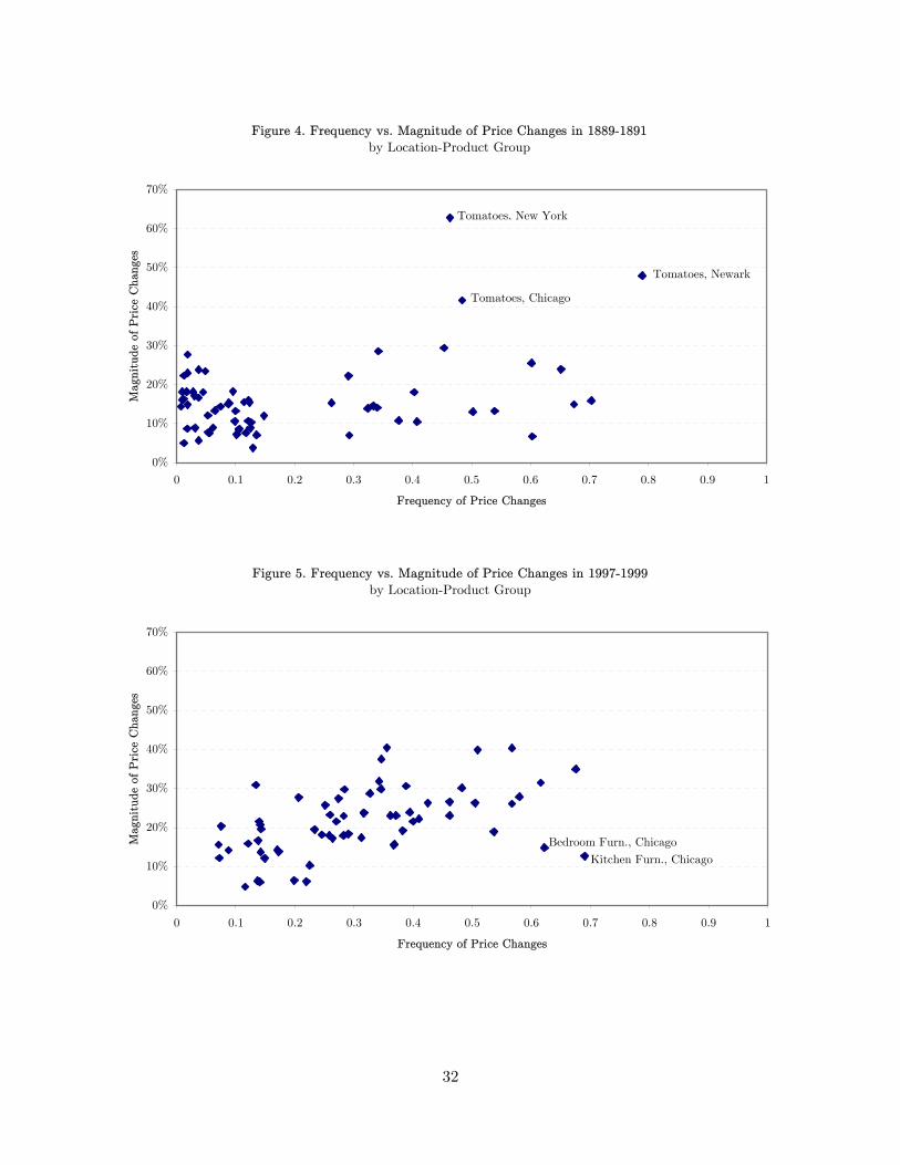
In both periods products that changed price more often were more likely to have slightly
larger price changes. The relationship between the frequency and size of price changes is plotted
in figures 4 and 5 using observations grouped by location and product. The positive relationship
between the frequency and size of price changes is more robust in 1997-1999 than it is in 1889-
1891. In the earlier data, the positive correlation is almost entirely driven by the price of
tomatoes.
As with the frequency of price changes, the change in the magnitude of price changes is
consistent across different ways of looking at the data. In each method of slicing the data, the
magnitude of price changes was somewhat lower in 1889-1891 than in 1997-1999.
Fewer very small price changes
Even though the average magnitude of prices changes may have been lower in 1889-1891
than in 1997-1999 there appears to have been fewer very small price changes in 1889-1891.
Pooling all price changes together, the cumulative distribution of the size of price changes is
shown in figure 6. A noticeable trait of the 1889-1891 data is the fairly sharp change in the
slope of the cumulative distribution as the size of the change approaches zero. The flatness
suggests price changes that are a small amount of the good’s price are avoided.19 This behavior
is predicted by a cost to changing prices, such as a menu cost. In 1997-1999 there is little
observable flatness around zero, suggesting price changes less than a couple percent in size were
no less likely to occur than price changes a few percentage points larger.
18 Changing the threshold from three or more observations substantially changes the number of possible cell comparisons, but has little effect on the share of cells for which the magnitude of price changes increased. 19 It should be emphasized that “small” is defined in terms of the percentage change in the good’s price. As noted earlier, the size of price changes in dollar terms has increased as a result of the around 6,000 percent increase in overall prices that occurred over the 118 years between the two time periods.

11
The paucity of small price changes in 1889-1891 is even more apparent in figure 7. This
figure displays the share of price changes (vertical axis) less than a given absolute size (the
horizontal axis). In 1889-1891 the share of price changes that were less than 2.5 percent in
magnitude was less than a fifth the share in 1997-1999. Also, almost no price changes in the
earlier period were less than 1.5 percent in magnitude. Such small price changes were not
uncommon in the 1997-1999 period.
Monetary indivisibility is an alternative to a price changing cost for explaining the lack
of small price changes in 1889-1891. Despite the large change in the price level since 1889, the
smallest coin minted in the US in 1889 had the same nominal value as the smallest coin
currently minted–1-cent. This likely discouraged some merchants from making price changes
less than 1-cent in magnitude. However, in the 1889-1891 data, 2-cent and 5-cent price changes
were each slightly more common than 1-cent price changes, which would not be expected if
monetary indivisibility were significant problem.20 Further, with some of the goods in the earlier
period being sold in bulk, price changes less than 1-cent in size were not uncommon, about
7 percent of price changes in 1889-1891 were less than 1-cent in magnitude.
Less use of Temporary Price Reductions (Sales) and More Price Churning
Lal and Matutes (1994) cite a survey of supermarket managers suggesting temporary
price reductions became more important during the 1980s. How important are temporary price
reductions in explaining the higher frequency of price changes observed in 1997-1999?
Only one- and two-month temporary price reductions are considered in this paper. A
one-month temporary price reduction is defined as a drop in price perfectly counteracted the
following month.21 A two-month temporary price reduction is a drop in price taken back in
either one of the next two months.
It is possible that this definition of a temporary price reduction does not catch all short-
term sales of goods. For example, the definition would miss a good put on sale at a lower price
before moving to a new, higher-than-before “regular” price. But, using higher frequency data,
Warner and Barsky (1995) find 51 out 62 temporary price reductions in their sample were
20 In the 1889-1891 data, price changes that had a nominal value of 2-cents accounted for 20 percent of the price changes, followed by 5-cents (19 percent of price changes), 1-cent (17 percent), 3-cents (10 percent), 1/2-cent (5 percent), and 10-cents (5 percent). 21 The price in month two is less than in month one, but in month three it returns to the price in month one. Observations where a reduction in price occurred in the last sampled month are dropped since it is impossible to determine if the price change was a temporary price reduction or a more permanent price reduction. Hosken, Matsa, and Reiffen (2000) use a similar definition.

12
exactly reversed, suggesting that this definition of temporary price reductions probably catches
most sales.
Similar to temporary price reductions are price markdowns. Price markdowns start with
a high initial price that is gradually reduced over time. Markdowns differ from temporary price
reductions in that the price never increases until the product is sold out. They are common in
goods for which fads or fashions change quickly and production runs are short.22 Few of the
product groups in the sample fit this description and therefore significant effects from price
markdowns are unlikely.
Table 5 shows the frequency and size of price changes for a pooling of all observations
before and after filtering out various combinations of price markdowns and temporary price
reductions. Filtering out temporary price reductions decreases the frequency of price changes
much more in 1997-1999 than in 1889-1891, suggesting an increase in the use of temporary price
reductions. About 15 percent of price changes in 1889-1891 were either a temporary price
reduction or the reversal of the price reduction, compared with 40 percent in 1997-1999.
Nonetheless, even excluding temporary price reductions and price markdowns, price changes
were at least four times more common in 1997-1999 than in 1889-1891.
Excluding price markdowns and temporary price reductions has less effect on the
magnitude of price changes. Removing temporary price reductions decreases the magnitude of
price changes about 2 to 3 percent in 1997-1999, suggesting that temporary price reductions
during that period were somewhat larger in magnitude than normal price changes. In contrast,
removing temporary price reductions has a negligible effect on the average magnitude of price
changes in 1889-1891.
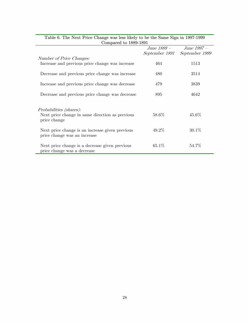
An alternative view of temporary price changes can be seen by looking at the probability
of two consecutive price changes of the same sign. In a standard S-s pricing model with
permanent shocks to the optimal price, and no trend drift rate in the optimal price, the
probability of the next price change being in the same direction as the previous price change is
50 percent. If there is a trend drift rate in the optimal price, this probability will be higher than
50 percent, whereas if changes in the optimal price are temporary the probability may be below
50 percent. In the 1889-1891 period, the next price change was somewhat more likely to be in
the same direction as the previous price change, while consecutive price changes were less likely
to be in the same direction in 1997-1999. (Table 6.) This finding suggests that price changes
were more permanent in 1889-1891 than they were in 1997-1999.

13
Discussion To understand the potential causes of the differences in price adjustment in 1889-1891
and 1997-1999, it is useful to summarize some of the major changes that have taken place in the
retailing environment during the last century.23
First, stores today are much larger than they were in the late 1880s, both in the number
of employees and in the number of goods offered for sale. In 1889-1891 most stores were quite
small and concentrated on a few products. For example, in 1889 the grocery chain A&P sold
mostly tea, coffee, butter, sugar and baking powder.24 By 1928, the number of items carried by
the average grocery store increased to 867. This jumped to around 3,000 items in each store in
1946 and to 6,800 in 1963.25 Today, conventional supermarkets carry around 25,000 items and
include a bakery, a meat counter, and a large selection of non-food items.26 Measuring store size
by the number of employees shows a similar increase. Quantitative information for 1890 is
scare, but Nystrom (1919, 1930) suggests that stores were usually a one or two man operation.
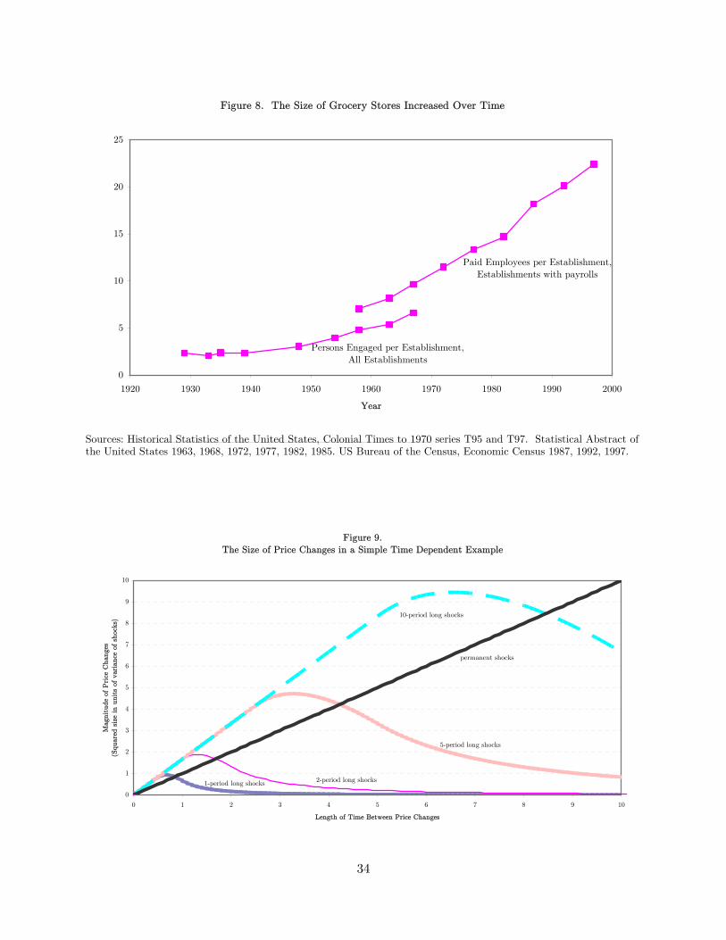
The increase in the size of supermarkets since 1929, when quantitative figures first became
available, can be seen in Figure 8, which displays employees per food retailer. By this measure
the size of grocery stores increased almost tenfold between 1929 and 1997.
Another difference between retailing in 1889-1891 and 1997-1999 is that the industry is
much more concentrated today. Although there were exceptions with a few large department
stores in New York (Macy’s, Lord & Taylor, and Bloomingdale’s) and Chicago (Marshall
Fields), the retail business was fragmented in 1890. Only six grocery chains, one drug chain,
and ten other retail chains were operating in the United States in 1890.27 A&P, the largest of
these chains, owned over a hundred grocery stores scattered throughout the eastern half of the
U.S. However, even in its largest market, New York, A&P operated only about 25 stores.28
Kroger, a grocery chain based in Cincinnati, operated only seven stores in 1890.29 Barger (1955)
estimates that chain stores held a miniscule fraction of grocery business in the U.S. before
22 Pashigian (1988) 23 This section concentrates on the food retailing industry, since most of the products used in this study are sold in supermarkets, but the broad outline should be applicable to changes throughout the retail goods industry. 24 Bullock (1933) p. 61-62. While the stores sold only a few types of products, they would typically carry several varieties of each product. 25 National Commission on Food Marketing (1966) p.2. The head of Kroger cites similar figures in Hall (1957) p.26. 26 Food Marketing Institute. Supermarket Facts: Industry Overview 2001 (http://www.fmi.org/facts_figs/superfact.htm) 27 A chain is defined as two or more stores under the same management. Historical Statistics of the United States p.836 and 847. 28 Bullock (1933) p.61-62

14
1900.30 Since this earlier time chain stores have accounted for an ever-rising share of the grocery
industry. Chain stores’ share of grocery sales rose from around 20 percent of the grocery
business in 1909 to 40 percent in the mid-1930s to over 70 percent during the 1980s.31
A third difference in the retailing environment is the weakening of the personal
relationship between the retailer and customer. In 1889-1891, with most retailing occurring in
small shops, a relationship existed between the retailer and the customer. Part of this
relationship was probably personal. Without refrigerators, grocery shopping was done nearly
every day. And, being a one or two-man store, the shopkeeper probably got to know his
customers personally. Another part of the relationship may have been brought on by business
concerns. For instance, the retailer often supplied credit to the customer, and the inability to
collect on this credit was the downfall of many grocery stores. Because transportation was
difficult and carrying purchases was burdensome, retailers usually delivered the purchases to the
customer’s home at no extra charge. This gave customers a reason to stay loyal to the retailer.
Regular customers might be placed near the beginning of a delivery route, getting the butter
when it was still hard, while customers with less of a relationship might not get their goods until
the end of the delivery route, when the butter was getting soft. The importance of the retail
relationship in the late-1800s was noted by the editor of the American Grocer in 1896:
The grocery business is, perhaps more than any other, dependent for success or failure upon the individuality of the man engaged in it, even more than his business methods. If he wins the confidence of customers by keeping only good things, selling them at reasonable prices, being obliging and prompt in his deliveries and is reasonably careful about given credits, he will command and hold patronage.32 The few surveys available document declining customer loyalty to a particular store over
the last century. The percentage of supermarket shoppers patronizing one store exclusively fell
substantially in the post-war years, from 41 percent in 1954 to 29 percent in 1961 to 17 percent
in 1965.33 More recently, shoppers have become more willing to change the supermarket where
they do most of their shopping. The percentage of shoppers changing their supermarket in the
past year jumped from 18.2 percent in 1979-1980 to between 24 and 27 percent from 1990 to
29 Lebhar (1963) p.396 30 Barger (1955, p. 148); 31 Barger (1955, p. 148), Chain Store Age (1950) p.J3. Nielsen (1985, 1989 p.4). 32 New York Daily Tribune, October 11, 1896, (sect III, p15, col7) 33 Schapker (1966). Table 1, p. 47. While the surveys continued for a number of additional years, the question seems to have been dropped.

15
1994. In almost all years, the main reason for switching stores was lower prices at the new
store.34
A final difference in the retail environment is that the share of income spent on the
goods covered in this study has declined substantially. Although food goods make up most of
the observations in this study, the share of food in consumer expenditures has dropped from 40
percent in 1889-1891 to approximately 10 percent in 1997-1999.
These four changes in retailing structure (larger stores, greater industry concentration,
declining customer-retailer relationship, and declining importance of food) have probably
reduced the cost to changing prices. Larger stores, by carrying more products and employees,
can exploit economies of scale in changing prices. Empirically, Buckle and Carlson (2000) find
larger firms change prices more often. Similarly, the increase in industry concentration may also
have lowered the cost of changing prices because many chain store pricing decisions are made
above the store level. This allows the managerial costs of deciding when and by how much to
change prices to be spread across many stores. Ball and Mankiw (1994) suggest that managerial
costs are much larger than menu costs, a point echoed in the empirical work of Zbaracki, et al.
(2004). The decline in the relationship between the retailer and the customer and the decline in
the importance of food in consumers’ expenditures also effectively lowered the cost of changing
prices by lessening the chance of, in Patton’s (1889) words, “arousing the indignation” of
customers and thereby losing their business when price increases occurred.
If the cost of changing prices was higher in 1889-1891 than in 1997-1999 most standard
models of price adjustment would find the less frequent price changes and fewer “small” price
changes that were observed in the data. But, standard pricing models with permanent shocks
would not predict the smaller average magnitude of price changes observed in 1889-1891, or the
use of temporary price reductions that have become more prevalent in the recent period.
We can reconcile these last two findings if we assume that a significant share of the
shocks to the profit maximizing price are temporary. Take a simple time-dependent pricing
example: Assume the optimal price follows a moving average of independent standard normal
shocks, 1*t t tp µ µ −= + . By definition, the firm would charge the optimal price in a perfectly
frictionless world. However, say that the firm must pay a cost, C , to see the realized value of
the shocks and the resulting optimal price. In practice, this cost could come about because the
firm must expend labor to interpret the effect of changes in supply costs or customer buying
34 Burgoyne (1980), Food Marketing Institute (1994). These are the only surveys I have found asking this question. In one year, 1990, the top reason for switching grocery stores was that the new store was closer or had a more convenient location, possibly the result of a move by the respondent.
16
habits on the price the firm should charge. In other words, the cost, C, is an administrative
cost of determining the best price to charge, and not a true menu cost. After paying the price
determination cost, there is no additional cost to changing prices. Once the firm pays the cost
C, they observe the shock to the optimal price and then set the price for the current period, pt.
They continue to charge the price pt until the next time the firm pays the cost to observe the
optimal price. Finally, the per period loss from maintaining a price that deviates from the
optimal price is the square of the deviation, 2( * )tp p− , and there is no inflation or other
discounting of losses.
Assume that the firm initially chooses to observe the optimal price every third period,
and changes their price every time the optimal price is observed. The frequency of price
changes is then 1/3. To minimize the per period loss, the firm will set the actual price to the
average expected optimal price. With the firm changing price every third period, this is:
0 0 0 1 0 2( * ) ( * ) ( * ) 1 2 10 0 0 1 0 1 0 0 2 1 0 13 3 3 3( ( ) ( ) ( ))E p E p E pp E E Eµ µ µ µ µ µ µ µ+ +
− −= = + + + + + = + ,
where the last equality occurs because shocks are mean-zero in expectation. Given this actual
price, the expected magnitude of price changes (measured here by the expected squared size of
price changes) is:
2 2 22 1 2 1 13 0 3 2 0 13 3 3 3 9( ) (( ) ( )) 1E p p E µµ µ µ µ σ−− = + − + = .
Finally, the expected average per period loss from having a constant price plus the cost
of changing prices is 2 2 2
0 0 0 1 0 2(( * ) ( * ) ( * ) ) 2123 3 27 31E p p p p p p C C
µσ− + − + − + = + .
Next, assume the firm changes price every other period. The frequency of price changes
then increases to 1/2. The firm will set its actual price to the average expected optimal price in
the next two periods: * *
0 0 0 1( ) ( ) 1 10 0 0 1 0 1 0 0 12 2 2( ( ) ( ))E p E pp E Eµ µ µ µ µ µ+
− −= = + + + = + . The
expected per period loss from following this policy of changing price every other period is * 2 * 2
0 0 0 1(( ) ( ) ) 212 2 4 21E p p p p C C
µσ− + − + = + , which is lower than the cost of changing prices every third
period if 267
C
µσ< . This suggests that, for a given size of temporary shocks, a lower cost of price
changes will increase the frequency of price changes, a result that occurs in nearly all price
setting models. However, the expected size of price changes when the changing price every
other period is 2 2 21 1 12 0 2 1 0 12 2 2( ) (( ) ( )) 2E p p E µµ µ µ µ σ−− = + − + = , which is larger than the
size of price changes when setting price every third period. When price changes become more
frequent, price changes become larger because firms now follow the up and down patterns that
occur with temporary shocks rather than smoothing through the short-run volatility. The

17
transitory shocks will also lead to the more temporary nature of price changes seen in the 1997-
1999 data.
Figure 9 shows how the size of price changes relates to the persistence of shocks in a
version of this time-dependent example where shocks occur continuously and time between price
changes is also allowed to vary continuously. When shocks to the optimal price are permanent,
reducing the time between price changes always leads to a decrease in the magnitude of price
changes. On the other hand, when shocks to the optimal price are temporary, reducing the time
between price changes leads to an increase in the magnitude of price changes if the initial time
between price changes is relatively long. The intuition behind this result is that when shocks
are temporary, and the length of time between price changes is long, little attention is paid to
the current shocks in setting the price because the shocks will be long gone by the time of the
next price change.
One additional feature of this simple model is that magnitude of price changes can be
larger when shocks are temporary than when shocks are permanent. Consider the discrete-time
example, but now with permanent shocks. In this case, when changing their price the firm will
set it equal to the current optimal price. When changing price every other period this implies
that the expected size of price changes is:
2 2 2 22 0 2 0 0 2 1 0( ) ( * * ) (( * ) * ) 2E p p E p p E p p µµ µ σ− = − = + + − =
which is smaller than the 2122 µσ size of price changes that occurred when shocks were
temporary and firms changed price every other period.
That temporary shocks can sometimes lead to larger price changes than permanent
shocks is also visible in figure 9. If shock persistence is long relative to the time between price
changes, then temporary shocks will lead to larger price changes than will permanent shocks.
Larger price changes in response to temporary shocks is also consistent to what was found in the
data on table 5. There the size of price changes decreased when temporary price reductions
were filtered out of the 1997-1999 data.
Intuitively, temporary shocks can lead to larger price changes than permanent shocks
because temporary shocks create a more variable change in the optimal price over short-horizon.
When shocks are temporary, at any given instance a new shock occurs and an old shock
disappears, each of which adds variance to the change in the optimal price. When shocks are

18
permanent old shocks never disappear, and only new shocks perturb the optimal price making
short-term changes in the optimal price less variable.35
Before concluding, it should be emphasized that the results presented in this paper refer
to microdata prices not to aggregate prices. Changes in the cross-correlation of prices or
changes in the composition of output may make aggregate rigidity results different from those
found in this paper. For example, Hanes (1998, 1999) suggests that the economy has become
more processed over the last one hundred years. He also suggests (as do Bils and Klenow (2004)
and Thompson and Wilson (1999)) that processed goods are more rigid than unprocessed goods.
Conclusion That nominal price rigidity may have declined over time is suggested when comparing
the handful of previous studies and anecdotal evidence. On the other hand, this apparent
decline of nominal price rigidity could have been an artifact of inconsistencies in coverage and
sources across the different studies. The results presented here suggest this probably is not the
case, and nominal price rigidity likely has declined. Using consistent data in two periods widely
separated in time, this paper found nominal price rigidity in 1997-1999 was substantially less
than in 1889-1891. The decline in nominal price rigidity is robust across the goods, months, and
locations matched across the two periods. Further, the decline does not appear to be the result
of differences in aggregate inflation rates.
Additional findings include an increase in the average magnitude of price changes
between 1889-1891 and 1997-1999, though the difference between the two periods is less
dramatic than is the difference in nominal price rigidity. Finally, small price changes and
temporary price reductions have become more common in the recent period.
These findings are consistent with a model in which shocks to the optimal price are
transitory and in which the cost of changing prices decreased between 1889-1891 and 1997-1999.
The cost of changing prices likely fell between the two periods as a result of changes in the
retailing environment, which included larger stores, greater industry concentration, the declining
customer-retailer relationship, and the declining importance of food.
35 If the optimal price followed a mean-reverting autoregressive process, rather than a moving average process, then the expected size of price changes would converge to the permanent shock case as shocks became more persistent. This does not occur with the moving average shock example shown. Further, an analytically-intractable S-s model with temporary shocks is also likely to find that price changes in response to temporary shocks are larger than price changes in response to permanent shocks. This is because the additional profit (prior to deducting the cost of the price change) from a temporary price

19
In sum, from today’s perspective, Professor Patten’s age of highly variable prices looks
like the good old times of nominal price rigidity.
change would have to pay the menu cost twice (once for the price increase and once the price decrease) whereas the additional profit from a permanent price change would only have to pay the menu cost once.

20
References Aldrich, Nelson. (1892) Retail Prices and Wages. Committee on Finance. Senate. 52nd
Congress. 1st Session. Report 986. Washington, DC: U.S. Government Printing Office. Parts 1-3.
Backman, Jules. (1940) “The Causes of Price Inflexibility.” The Quarterly Journal of
Economics, Volume 54, Number 3. May, 474-489. Ball, Laurence and N. Gregory Mankiw. (1994) “A Sticky-Price Manifesto.” Carnegie Rochester
Conference Series on Public Policy. Volume 41. Number 0. December, 127-151. Barger, Harold. (1955) Distribution’s Place in the American Economy since 1869. National
Bureau of Economic Research. General series, no.58. Princeton University Press, Princeton.
Bezanson, Anne, Robert D. Gray, and Miriam Hussey. (1936) Wholesale Prices in Philadelphia
1784-1861. University of Pennsylvania Press. Philadelphia. Bils, Mark, and Peter Klenow. (2004) “Some Evidence on the Importance of Sticky Prices.”
Journal of Political Economy. 112 October, 947-985. Buckle, Robert A., and John A. Carlson. (2000) “Menu Costs, Firm Size and Price Rigidity.”
Economics Letters. Volume 66, Issue 1. January, 59-63. Bullock, Roy J. (1933) “History of the Great Atlantic & Pacific Tea Co. Since 1878.” Harvard
Business Review. Volume12, Number 1. October. Pp. 59-69 Burgoyne, Inc. (1980) National Study of Supermarket Shoppers (Census Profile) Cincinnati,
Ohio. Carlton, Dennis W. (1983) “Equilibrium Fluctuations when Price and Delivery Lag Clear the
Market.” The Bell Journal of Economics. Volume 14, Number 2. Autumn. pp. 562-572 Carlton, Dennis W. (1986) “The Rigidity of Prices.” American Economic Review. Volume 76,
Issue 4. September. Pp. 637-658. Reprinted in Sheshinski and Weiss (1993). Cecchetti, Stephen G. (1986) “The Frequency of Price Adjustment: A Study of the Newsstand
Prices of Magazines.” Journal of Econometrics. Volume 31 p.255-274. Reprinted in Sheshinski and Weiss (1993).
Chain Store Age. (1950) Grocery Manager’s edition. Lebhar-Friedman Publications. New York.
June. Consumer Reports. (2001) “Tissues disappear.” December. p.63. Dimand, Robert W. (2000). “Oskar Morgenstern on apparent price rigidity in the 1930s: a
comment on Kovenock and Widdows.” European Journal of Political Economy. Volume 16. pp.571-573.
21
Food Marketing Institute. (1980) Supermarket Trends. Washington DC. Research Division,
Food Marketing Institute. Food Marketing Institute. (1981, 1982, 1985, 1986, 1994) Trends - Consumer Attitudes and the
Supermarket. Washington DC. Research Division, Food Marketing Institute. Goodwin, Barry K., Thomas J. Grennes, and Lee A. Craig. (2002) “Mechanical Refrigeration
and the Integration of Perishable Commodity Markets.” Explorations in Economic History. Volume 39. Number 2. April. Pp. 154-82.
Hall, Joseph B. (1957) “Evolution not Revolution: The Present Job of Management in Food Distribution.” In The Tobe Lectures in Retail Distribution at the Harvard Business School. Second Series (1957-1958).
Hanes, Christopher. (1998) “Consistent Wholesale Price Series for the United States, 1860-
1990.” In Business Cycles Since 1820 ,Trevor J.O. Dick ed. Edward Elgar, Northampton, MA.
Hanes, Christopher. (1999) “Degrees of Processing and Changes in the Cyclical Behavior of
Prices in the United States, 1869-1990.” Journal of Money, Credit, and Banking. Volume 31, Number1. February. Pp. 35-53.
Hosken, Daniel, David Matsa, and David Reiffen. (2000). “How Do Retailers Adjust Prices?:
Evidence from Store-Level Data.” Federal Trade Commission Bureau of Economics Working Paper. January.
Kashyap, Anil K. (1995) “Sticky Prices: New Evidence from Retail Catalogs.” Quarterly
Journal of Economics. Pp. 245-274. Koelln, Kenneth, and Mark Rush. (1993) “Rigid Prices and Flexible Products.” Journal of
Economics. Missouri Valley Economic Association. Volume 19. Number 1. Spring. Pp. 57-64.
Lal, Rajiv, and Carmen Matutes. (1994) “Retail Pricing and Advertising Strategies.” Journal of
Business. Volume 67, Issue 3. July. Pp. 345-370. Lebhar, Godfrey M. (1963) Chain Stores in America: 1859-1962. Third Edition. Chain Store
Publishing Corporation. New York. Levy, Daniel, Mark Bergen, Shanantu Dutta, and Robert Venable. (1997) “The Magnitude of
Menu Costs: Direct Evidence From Large U.S. Supermarket Chains.” Quarterly Journal of Economics. August: Volume 112, Issue 3. Pp.791-825.
Levy, Daniel, and Andrew Young. (2004) “ ‘The Real Thing:’ Nominal Price Rigidity of the
Nickel Coke, 1886-1959.” Journal of Money, Credit, and Banking. August. Volume 36, Number 4. pp. 765-799
Mills, Frederick C., (1927) The Behavior of Prices. National Bureau of Economic Research. New
York.
22
Morgenstren, Oskar. (1931) “Free and fixed prices during the depression.” Harvard Business Review. Volume 10. pp. 62-63
National Commission on Food Marketing, United States. (1966). Food from Farmer to
Consumer. U.S. Government Printing Office. Washington. Neilsen, A.C., Company (1985, 1989) Nielsen Annual Review of Retail Grocery Store Trends.
Hackensack, NJ. Nystrom, Paul H. (1919) Economics of Retailing. The Ronald press company. New York. Nystrom, Paul H. (1930) Economics of Retailing. 3d ed. The Ronald press company. New York. Pashigian, B. Peter. (1988) “Demand Uncertainty and Sales: A Study of Fashion and Markdown
Pricing.” American Economic Review. Volume 78, Issue 5. December pp.936-953. Patten, Simon N. (1889) “The Stability of Prices.” Publications of the American Economic
Association. Volume III. Number 6. January. Powers, Elizabeth T., and Nicholas J. Powers. (2001) “The Size and Frequency of Price
Changes: Evidence from Grocery Stores.” Review of Industrial Organization. Volume 18, Number 4. June 2001. Pp 397-416.
Schapker, Ben L. (1966) “Behavior Patterns of Supermarket Shoppers.” Journal of Marketing.
October. Pp.46-49. Stigler, George J., and James K. Kindahl. (1973) “ Industrial Prices, as Administered by Dr.
Means.” American Economic Review. Volume 63, Issue 4. Pp. 717-721. Taylor, John B. (1999) “Staggered Price and Wage Setting in Macroeconomics.” In Handbook of
Macroeconomics Volume 1B. John B. Taylor and Michael Woodford Eds. Elsevier. Amsterdam.
Thompson, Gary D., and Paul N. Wilson (1999) “Market Demands for Bagged, Refrigerated
Salads.” Journal of Agricultural and Resource Economics. Volume 24. Number 2. December. Pp. 463-81.
United States Bureau of Labor Statistics. (various dates between 1911 and 1916) Retail Prices.
Retail Prices and Cost of Living Series. BLS Bulletins 105, 106, 108, 110, 113, 115,125, 132, 136, 138.
United States Department of Agriculture, Economic Research Service. (1966) Retail Prices of
Selected Foods in Two North Carolina Areas, July 1962-June 1963. Warner, Elizabeth J., and Robert B. Barsky. (1995) “The Timing and Magnitude of Retail
Store Markdowns: Evidence from Weekends and Holidays.” Quarterly Journal of Economics. Volume 110, Issue 2. May. Pp. 321-52.
Warren, G.F. and Pearson, F.A. Wholesale Prices for 213 Years, 1720 to 1932: Part I. Whole
sale Prices in the United States for 135 Years, 1797 to 1932. Cornell University, Agricultural Experiment Station. Memoir 142. Ithaca, New York. 1932.

23
Zbaracki, Mark J., Mark Ritson, Daniel Levy, Shantanu Dutta, and Mark Bergen. (2004)
“Managerial and Customer Costs of Price Adjustment: Direct Evidence from Industrial Markets.” Review of Economics and Statistics. Volume 86. Issue 2. May. pp. 514-33.
24
Table 1. Selected Prior Microdata Estimates of the Length of Nominal Rigidity
Estimated Length of Nominal Rigidity
Average Absolute Size of
Change
Period of Coverage
Type of Good Study
73 years - 1886-1959 Coca-Cola Levy and Young (2004)
1.8 to 14 years 14.3 to 29.4% 1953-1979 Magazine Cover
Prices
Cecchetti (1986)
11.2 to 30 months 5 to 17% 1953-1987 Catalog Apparel and Outdoor Accessories
Kashyap (1995)
3.6 to 13.2 months 0.8 to 7.7% 1957-1966 Wholesale Industrial Prices
Carlton (1986)
4.3 months36 - 1995-1997 Consumer Goods Bils and Klenow (2002)
3.0 months37 2.7 months 2.5 months 2.0 months
- 1791-1810 1811-1830 1821-1840 1841-1860
Wholesale Prices in Philadelphia
Bezanson, et al. (1936)
2.8 months38 2.6 months 3.2 months 2.1 months 1.9 months
- 1890-1897 1898-1905 1906-1913 1914-1921 1922-1925
Wholesale Commodity Prices
Mills (1927)
4.5 to 15 weeks - 1991-1992 Prices in Supermarket chains
Levy, et al. (1997)
2.3 weeks 24% 1986-1992 Lettuce in grocery stores
Powers and Powers (2001)
36 Median length 37 Approximated from Bezanson, et al. (1936) chart VI p. 55. 38 Inverse of median commodity frequency of price change from appendix table VIII.

25
Table 2. A Comparison of Selected Fundamentals in the Three Periods
June 1889— September 1891
June 1997— September 1999
Average Annual Wholesale Price Inflation Rate39
0.00% 0.28%
Nearby or Included Business Cycle Dates40 April 1888 Trough July 1890 Peak
May 1891 Trough January 1893 Peak
March 1991 Trough March 2001 Peak
Interest rate41 4.57% 6.79%
Table 3. 48 Products Are Available in 1889-1891 and 1997-1999 Food Goods Household goods, furniture,
and hardware Clothing
1. Beef Roasts 1. Laundry Starch 1. Men’s underwear 2. Ham 2. Cleaning Products 2. Men’s Socks 3. Eggs 3. Stoves and ovens 3. Men’s shirts 4. Bacon 4. Kitchen table, chair and sets 4. Women’s pantyhose and stockings 5. Sugar 5. Dining room furniture 5. Waterproof Footwear 6. Butter and Margarine 6. Bedroom furniture 6. Men’s work shoes and boots 7. Potatoes 7. Drinking Glasses 7. Women’s dress and casual shoes 8. Milk 8. Knives and Forks 9. Flour 9. Kitchen Knives 10. Lard 10. Dishes 11. Cornmeal 11. Nonelectric cookingware 12. Mutton 12. Shovels 13. Bread 13. Rope 14. Turkey (excluding canned) 14. Saws, axes, and hammers 15. Tomatoes 16. Canned Fruit 17. Salt and other seasonings 18. Beer 19. Rice 20. Canned Fish 21. Cheese 22. Coffee 23. Tea 24. Dried Beans 25. Dried Fruits 26. Fresh Vegetables 27. Canned vegetables
39 1889-1891 from Warren and Pearson (1932), Table 1. 1997-1999 from Bureau of Labor Statistics, Producer Price Index, All Commodities. 40 NBER (http://www.nber.org/cycles.html) 41 Moody’s AAA Corporate Bond Yield. Calculated as geometric mean of closing yield on last day of month. Data from Global Financial Data (www.globalfindata.com).

26
Unweighted Average Absolute Size of Non-zero First Differences of Log Price
16.1% 24.9%
Unweighted Average of the Annualized First Difference of Log Price
0.07% -0.93%
Table 4. Comparative Data Set Statistics June 1889 —
September 1891 June 1997 —
September 1999
Total Number of First Differences
45,683 40,474
Number of Price Changes 2,367 12,709
Average Number of First Differences per Month
1,692 1,499
Average Observed Consecutive First Differences (maximum 27)
24.5 9.9
Average Number of First Differences per Product Group in a Location
246.9 238.1
Share of First-Differences that are Food Goods 54% 83%
Share of Price Changes that are Price Increases 52.8 52.2

27
Table 5. Filtering Out Temporary Price Reductions and Price Markdowns (All Observations - Unweighted Data)
June 1889 —
September 1891 June 1997 —
September 1999
Frequency of Price Changes (Share of Goods Changing Price Each Month) Unfiltered data
5.2% 31.4%
1-Month Temporary Price Reductions Filtered Out
4.8% 22.4%
2-Month Temporary Price Reductions Filtered Out
4.4% 18.9%
Price Markdowns and 1-Month Temporary Price Reductions Filtered Out
4.6% 22.1%
Price Markdowns and 2-Month Temporary Price Reductions Filtered Out
4.3% 18.7%
Magnitude of Price Changes
Unfiltered data 16.1% 24.9%
1-Month Temporary Price Reductions Filtered Out 16.3% 22.9%
2-Month Temporary Price Reductions Filtered Out 16.1% 22.0%
Price Markdowns and 1-Month Temporary Price Reductions Filtered Out
16.4% 22.9%
Price Markdowns and 2-Month Temporary Price Reductions Filtered Out
16.3% 22.1%
28
Table 6. The Next Price Change was less likely to be the Same Sign in 1997-1999
Compared to 1889-1891 June 1889 —
September 1891 June 1997 —
September 1999 Number of Price Changes: Increase and previous price change was increase
464 1513
Decrease and previous price change was increase
480 3514
Increase and previous price change was decrease
479 3839
Decrease and previous price change was decrease
895 4642
Probabilities (shares): Next price change in same direction as previous price change
58.6% 45.6%
Next price change is an increase given previous price change was an increase
49.2% 30.1%
Next price change is a decrease given previous price change was a decrease
65.1% 54.7%

29
Figure 1A. Frequency of Price Changes by Product
0%
10%
20%
30%
40%
50%
60%
Suga
rEg
gs
Potatoe
s
Butter
Shortening
Tomatoes
Dried fru
it
Canne
d fru
it
Cornm
eal
Dried be
ansFl
our
Salt
and season
ings
Rice
Mut
ton
Canne
d ve
getables
Tea
Bread
Coffee
Canne
d fis
hBee
rHam
Turke
y
Cheese
Bacon
Milk
Beef r
oasts
Misc
. fresh
veg
etab
lesRop
e
Shov
els
Tablew
are
Saws
Cookin
gware
Laun
dry sta
rch
Dishes
Flatwar
e
Cleaning
produ
cts
Stov
es and
Ove
ns
Glassw
are
Bedroom
furn
iture
Dining room
furn
.
Kitche
n furn
iture
Wom
en's
stock
ings
Wom
en's
shoe
s
Men
's shirt
s
Men
's sock
s
Men
's un
derw
ear
Waterpr
oof foo
twea
r
Men
's sh
oes
Num
ber
of P
rice
Cha
nges
/ N
umbe
r of
Obs
erva
tion
s
1889-1891 1997-1999
--------------Household---------------------------------------------------Foods------------------------------------- -----Clothing-----
Figure 1B. Frequency of Price Changes by Location
0%
10%
20%
30%
40%
New York Newark Chicago Los Angeles
City
Num
ber
of P
rice
Cha
nges
/ N
umbe
r of
Obs
erva
tion
s
1889-1891 1997-1999
Figure 1C. Frequency of Price Changes by Month
0%
10%
20%
30%
40%
July October January April July October January April July
Month
Num
ber
of P
rice
Cha
nges
/ N
umbe
r of
Obs
erva
tion
s
1889-1891 1997-1999
----------1889 & 1997---------- ------------------------------1890 & 1998------------------------------ --------------------1891 & 1999--------------------
30
Figure 2. The Probability of a Price Remaining Unchanged is Higher in 1889-1891(Kaplan-Meier Survival Function - All Observations - Unweighted)
0%
20%
40%
60%
80%
100%
0 5 10 15 20 25
Months
Shar
e of
Pri
ces
Not
Cha
nged
in
Num
ber
of M
onth
s
1997-1999
1889-1891

31
Figure 3A. Magnitude of Price Changes by Product
0%
10%
20%
30%
40%
50%
60%
Suga
rEg
gs
Potatoes
Butter
Shortening
Tomatoe
s
Dried fru
it
Canne
d fru
it
Cornm
eal
Dried be
ans
Flou
r
Salt
and season
ings
Rice
Mutton
Canne
d ve
getables
Tea
Coffee
Canne
d Fi
shHam
Cheese
Bacon
Milk
Beef R
oasts
Misc
. fresh
veg
etab
les
Cookin
gware
Dishes
Cleaning
produ
cts
Stov
es and
Ove
ns
Glassw
are
Bedroom
furn
iture
Dining room
furn.
Kitche
n furn
iture
Wom
en's
stock
ings
Men
's So
cks
Men
's Und
erwea
r
Men
's sh
oes
Ave
rage
abs
(ln(
p t/p
t-1)
)w
here
pt no
t eq
ual to
pt-
1
1889-1891 1997-1999
-------------------------------------------------------Foods------------------------------------------------------- -----------Household----------- ---Clothing---
Figure 3B. Magnitude of Price Changes by Location
0%
10%
20%
30%
New York Newark Chicago Los Angeles
City
Ave
rage
abs
(ln(
p t/p
t-1)
)w
here
pt no
t eq
ual to
pt-
1
1889-1891 1997-1999
Figure 3C. Magnitude of Price Changes by Month
0%
10%
20%
30%
July October January April July October January April July
Month
Ave
rage
abs
(ln(
p t/p
t-1)
)w
here
pt no
t eq
ual to
pt-
1
1889-1891 1997-1999
-------------------------------1890 & 1998------------------------------------------1889 & 1997---------- --------------------1891 & 1999--------------------
32
Figure 4. Frequency vs. Magnitude of Price Changes in 1889-1891by Location-Product Group
0%
10%
20%
30%
40%
50%
60%
70%
0 0.1 0.2 0.3 0.4 0.5 0.6 0.7 0.8 0.9 1
Frequency of Price Changes
Mag
nitu
de o
f P
rice
Cha
nges
Tomatoes, Chicago
Tomatoes, New York
Tomatoes, Newark
Figure 5. Frequency vs. Magnitude of Price Changes in 1997-1999by Location-Product Group
0%
10%
20%
30%
40%
50%
60%
70%
0 0.1 0.2 0.3 0.4 0.5 0.6 0.7 0.8 0.9 1
Frequency of Price Changes
Mag
nitu
de o
f P
rice
Cha
nges
Bedroom Furn., Chicago
Kitchen Furn., Chicago

33
Figure 6. Cumulative Distribution of Size of Price Changes
0%
10%
20%
30%
40%
50%
60%
70%
80%
90%
100%
-100% -80% -60% -40% -20% 0% 20% 40% 60% 80% 100%
Log Size of Price Change
Cum
ulat
ive
Sha
re
1997-1999
1889-1891
Figure 7. Small Price Changes Were Less Common in 1889-1891
0%
1%
2%
3%
4%
5%
6%
7%
0.0% 0.5% 1.0% 1.5% 2.0% 2.5% 3.0% 3.5%
Absolute Log Size of Price Change
Cum
ulat
ive
Shar
e of
Pri
ce C
hang
es
1997-1999
1889-1891
34
Figure 8. The Size of Grocery Stores Increased Over Time
0
5
10
15
20
25
1920 1930 1940 1950 1960 1970 1980 1990 2000
Year
Persons Engaged per Establishment,All Establishments
Paid Employees per Establishment,Establishments with payrolls
Sources: Historical Statistics of the United States, Colonial Times to 1970 series T95 and T97. Statistical Abstract of the United States 1963, 1968, 1972, 1977, 1982, 1985. US Bureau of the Census, Economic Census 1987, 1992, 1997.
Figure 9. The Size of Price Changes in a Simple Time Dependent Example
0
1
2
3
4
5
6
7
8
9
10
0 1 2 3 4 5 6 7 8 9 10
Length of Time Between Price Changes
Mag
nit
ude
of P
rice
Chan
ges
(Squ
ared
siz
e in
unit
s of
var
iance
of
shoc
ks)
permanent shocks
10-period long shocks
5-period long shocks
2-period long shocks1-period long shocks

35
Data Appendix To my knowledge there are only four sources for historical monthly time-series of retail
price microdata for the United States.42 The four sources are: 1. The Aldrich report (Aldrich,
1892) covering data from June 1889 to September 1891; 2. Various Bureau of Labor Statistics
bulletins (United States Bureau of Labor Statistics, various dates) covering retail prices of 12 to
18 foods in a number of cities from 1911 to 1916; 3. Retail Prices of Selected Foods in Two
North Carolina Cities, July 1962 to June 1963 (USDA, 1966); and, 4. The underlying data from
the Consumer Price Index (CPI) since the mid-1980s, which is available only by special
arrangement at the BLS office in Washington DC. The North Carolina food prices for 1962-
1963 were not used in this study, because the cities covered are not sampled monthly in either
the Aldrich report or the CPI. The 1911-1916 BLS data is also not used because the number of
goods covered is much smaller than either Aldrich report or the CPI sample, and the
macroeconomic conditions (i.e. higher inflation and war starting in 1914) differed from the other
two periods.
The microdata for 1889-1891 is extracted from exhibits appended to the Aldrich report
[Aldrich (1892)], an exhaustive study of retail and wholesale prices conducted by the then
recently formed Bureau of Labor Statistics under the direction of the Senate Finance committee.
The Aldrich Report was one of the first official attempts by an office of the government to
determine the course of prices and wages in the United States. Quoting approximately 115
products in each of 70 cities for 28 months, the breadth of coverage in Aldrich report would not
be matched by regular BLS sampling for at least 30 years.
After the Aldrich report regular BLS sampling of retail prices did not begin until 1903,
and even then comprised only food goods until 1917.43 Through a large number of pre-WWII
revisions and major post-war revisions in 1953, 1964, 1978, 1987, and 1998 the current consumer
price index evolved. Even with large changes in the product mix of the consumer’s basket over
the last one hundred and ten years, and enormous shifts in population distribution, some of the
goods and cities sampled in the Aldrich Report overlap with the sampling for today’s Consumer
Price Index.
42 It should be noted that there has been some innovative work in reconstructing time series of prices (for examplem magazine cover prices (Cecchetti, 1986) and catalog prices (Kashyap, 1995)). While a potentially longer time span of prices may be obtained this way, these sources are much more constrained in the frequency of quotes, the number of goods covered. Further, the data can not be used to compare differences across cities. 43 BLS Bulletin No. 699.
36
A series of interactions between the author and BLS personnel led to the formation a list
of goods and cities roughly comparable with the two different groups of data. This concordance
is given as Appendix Tables A1 and A2. After compilation of the data specifications, and a
required petition to the Commissioner of the BLS, the BLS provided screened 1997-1999
microdata for comparison with the Aldrich Report data.
In tailoring the 1997-1999 data to conform as closely as possible to the available data
from 1889-1891, beginning and ending dates were chosen to exactly match the length and
seasonality of the earlier data. Both sets of data begin in June and end 27 months later in
September. Products were chosen to maximize the number of comparable product groups
common to both samples. Localities were chosen to maximize the number of localities with
monthly sampling in both periods.
As I use microdata rather than a price index, the various CPI formula changes over the
years are not relevant and will not affect the results. The data in both periods were sampled by
trained BLS personnel bringing, hopefully, some degree of professionalism and uniformity to the
physical sampling, though the statistical techniques of determining what should be sampled
have changed tremendously over the time period. One change between the periods is the
disappearance of routine merchandise delivery by 1997-1999. Appendix Table A3 displays
additional methodological comparisons of the two periods.
One note of caution should be added. Both the geographic and product group
definitions are somewhat more inclusive in 1997-1999 than in the earlier period. For example,
the Aldrich Report sampled white beans. The narrowest available comparable product category
in the current data (a cluster within an entry level item) contains all dried beans, peas, and
lentils. Similarly, the 1889-1891 data sample Newark, New Jersey. The closest comparable
locality for the 1997-1999 dataset includes not only Essex county (where Newark is located) but
also the counties of Bergen, Hudson, Hunterdon, Mercer, Middlesex, Monmouth, Morris, Ocean,
Passaic, Somerset, Sussex, Union, Warren, as well as the county of Pike, Pennsylvania. More
comparisons between the 1889-1891 and the 1997-1999 groupings can be seen in Appendix
Tables A1 and A2. Given the increasing mobility of the population it is assumed the broader
groupings do not substantially alter the results.

37
Table A1. Geographical Correspondence Between 1889-1891 and 1997-1999 1889-1891 City Classification Current BLS Region Classification 1. Los Angeles, CA Los Angeles-Long-Beach, CA PMSA (A419) 2. Chicago, IL Chicago-Gary-Kenosha, IL-IN-WI CMSA
(Cook, DeKalb (starting 1998), DuPage, Grundy, Kane, Kankakee (starting 1998), Kendall, Lake, McHenry, and Will counties in Illinois; Lake and Porter counties in Indiana; and Kenosha county in Wisconsin) (A207)
3. New York, NY New York City (Bronx, Kings, New York, Queens, Richmond counties) (A109)
4. Newark, NJ New Jersey-Pennsylvania suburbs (Bergen, Essex, Hudson, Hunterdon, Mercer (starting 1998), Middlesex, Monmouth, Morris, Ocean, Passiac, Somerset, Sussex, Union and Warren (starting 1998) counties in New Jersey; and Pike county in Pennsylvania (starting 1998))(A111)
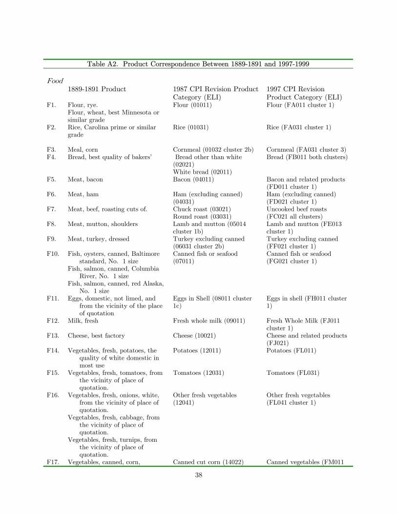
38
Table A2. Product Correspondence Between 1889-1891 and 1997-1999 Food 1889-1891 Product 1987 CPI Revision Product
Category (ELI) 1997 CPI Revision Product Category (ELI)
F1. Flour, rye. Flour, wheat, best Minnesota or similar grade
Flour (01011) Flour (FA011 cluster 1)
F2. Rice, Carolina prime or similar grade
Rice (01031)
Rice (FA031 cluster 1)
F3. Meal, corn Cornmeal (01032 cluster 2b) Cornmeal (FA031 cluster 3) F4. Bread, best quality of bakers’ Bread other than white
(02021) White bread (02011)
Bread (FB011 both clusters)
F5. Meat, bacon Bacon (04011) Bacon and related products (FD011 cluster 1)
F6. Meat, ham Ham (excluding canned) (04031)
Ham (excluding canned) (FD021 cluster 1)
F7. Meat, beef, roasting cuts of. Chuck roast (03021) Round roast (03031)
Uncooked beef roasts (FC021 all clusters)
F8. Meat, mutton, shoulders Lamb and mutton (05014 cluster 1b)
Lamb and mutton (FE013 cluster 1)
F9. Meat, turkey, dressed Turkey excluding canned (06031 cluster 2b)
Turkey excluding canned (FF021 cluster 1)
F10. Fish, oysters, canned, Baltimore standard, No. 1 size
Fish, salmon, canned, Columbia River, No. 1 size
Fish, salmon, canned, red Alaska, No. 1 size
Canned fish or seafood (07011)
Canned fish or seafood (FG021 cluster 1)
F11. Eggs, domestic, not limed, and from the vicinity of the place of quotation
Eggs in Shell (08011 cluster 1c)
Eggs in shell (FH011 cluster 1)
F12. Milk, fresh Fresh whole milk (09011) Fresh Whole Milk (FJ011 cluster 1)
F13. Cheese, best factory Cheese (10021) Cheese and related products (FJ021)
F14. Vegetables, fresh, potatoes, the quality of white domestic in most use
Potatoes (12011) Potatoes (FL011)
F15.
Vegetables, fresh, tomatoes, from the vicinity of place of quotation.
Tomatoes (12031) Tomatoes (FL031)
F16. Vegetables, fresh, onions, white, from the vicinity of place of quotation.
Vegetables, fresh, cabbage, from the vicinity of place of quotation.
Vegetables, fresh, turnips, from the vicinity of place of quotation.
Other fresh vegetables (12041)
Other fresh vegetables (FL041 cluster 1)
F17. Vegetables, canned, corn, Canned cut corn (14022) Canned vegetables (FM011

39
standard, No. 2 size. Vegetables, canned, pease,
standard, No. 2 size. Vegetables, canned, tomatoes, standard, No. 3 size.
Canned tomatoes and tomato juice (14023 cluster 2b) Other canned vegetables and vegetable juices (14023 cluster 4b)
cluster 2)
F18. Beans, white medium, best Dried beans (14023 cluster 3b)
Dried beans, peas, and lentils (FM031 cluster 2)
F19. Fruit, peaches, canned, No. 3 size, standard.
Canned Fruit (13031 cluster 1b)
Canned Fruit (FM011 cluster 1)
F20. Fruit, prunes, California. Fruit, prunes, Turkish. Fruit, raisins, California, medium quality. Fruit, raisins, Valencia. Fruit, currants, Zante. Fruit, apples, dried, good quality, evaporated.
Dried fruit (13031 cluster 2b) Dried and processed fruit (FM031 cluster 1)
F21. Coffee, Rio, fair, nonroasted Roasted Coffee (17031) Instant and Freeze Dried Coffee (17032)
Coffee (FP011) (both clusters)
F22.
Tea, Japan, medium grade. Tea, Oolong, medium grade.
Tea (17052) Tea (FP021)
F23. Sugar, standard granulated. Sugar and artificial sweeteners (15021)
Sugar and artificial sweeteners (FR011)
F24. Oleomargarine Butter, best creamery, excluding fancy grade Butter, best dairy, excluding fancy grade
Margarine (16011) Butter (10011)
Margarine (FS011 cluster 2) Butter (FS011 cluster 1)
F25. Lard, compound Lard, pure leaf
Lard and shortening (16012 cluster 1a)
Lard and shortening (FS032 cluster 1)
F26.
Salt, domestic, common fine. Salt, imported, best dairy. Spices, mustard, best domestic. Spices, nutmegs. No. 1. Spices, pepper, whole Singapore.
Salt and other seasonings and spices (18041)
Salt and other seasonings and spices (FT041)
F27. Beer Beer, ale, and other malt beverages at home (20011)
Beer, ale, and other malt beverages at home (FW011)
Household goods, furniture, and hardware 1889-1891 Product 1987 CPI Revision Product
Category (ELI) 1997 CPI Revision Product Category
H1. Starch, ordinary laundry. Laundry products (33012 cluster 1)
Laundry Products other than soaps and detergents (HN011 cluster 2)
H2. Ammonia, household. Cleaning products (33012 cluster 2)
Other cleaning products (HN011 cluster 3)
H3. Kitchen stoves and furnishings Stoves and ovens (excluding microwave ovens) (30031)
Stoves and ovens excluding microwave ovens (HK013)
H4. Furniture, chairs, kitchen, plain Kitchen table, chair and sets Kitchen table, chair and sets
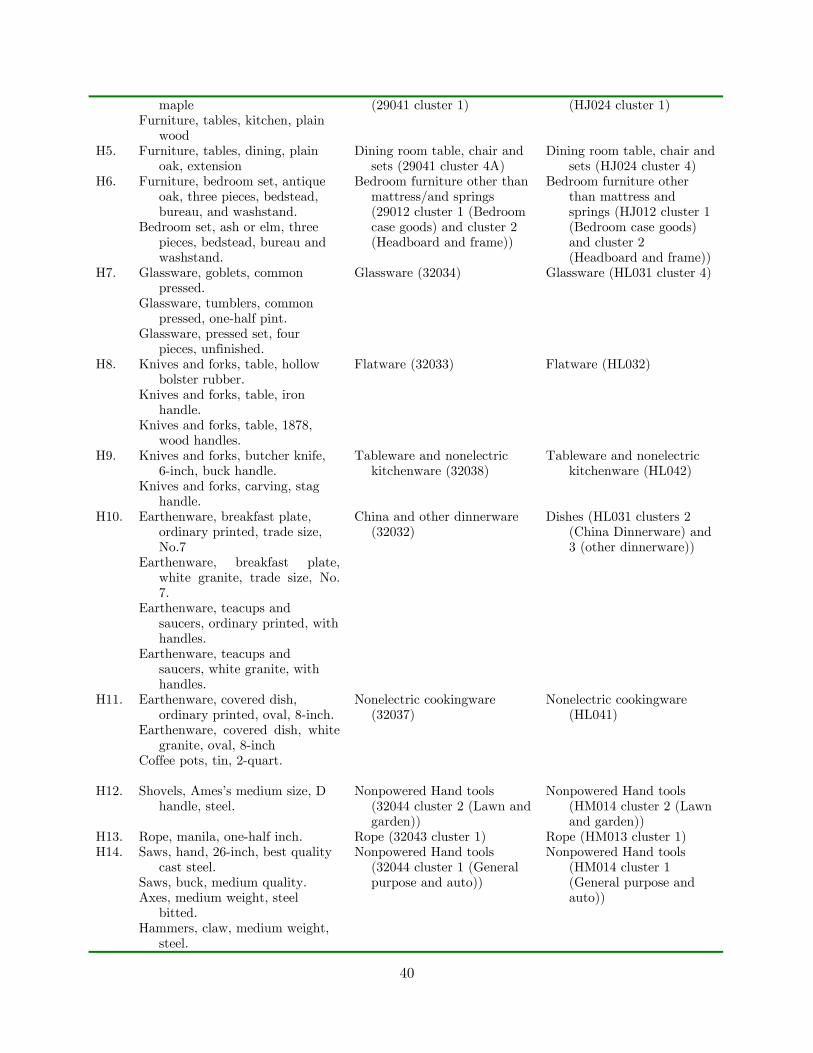
40
maple Furniture, tables, kitchen, plain
wood
(29041 cluster 1) (HJ024 cluster 1)
H5. Furniture, tables, dining, plain oak, extension
Dining room table, chair and sets (29041 cluster 4A)
Dining room table, chair and sets (HJ024 cluster 4)
H6. Furniture, bedroom set, antique oak, three pieces, bedstead, bureau, and washstand.
Bedroom set, ash or elm, three pieces, bedstead, bureau and washstand.
Bedroom furniture other than mattress/and springs (29012 cluster 1 (Bedroom case goods) and cluster 2 (Headboard and frame))
Bedroom furniture other than mattress and springs (HJ012 cluster 1 (Bedroom case goods) and cluster 2 (Headboard and frame))
H7. Glassware, goblets, common pressed.
Glassware, tumblers, common pressed, one-half pint.
Glassware, pressed set, four pieces, unfinished.
Glassware (32034) Glassware (HL031 cluster 4)
H8. Knives and forks, table, hollow bolster rubber.
Knives and forks, table, iron handle.
Knives and forks, table, 1878, wood handles.
Flatware (32033) Flatware (HL032)
H9. Knives and forks, butcher knife, 6-inch, buck handle.
Knives and forks, carving, stag handle.
Tableware and nonelectric kitchenware (32038)
Tableware and nonelectric kitchenware (HL042)
H10. Earthenware, breakfast plate, ordinary printed, trade size, No.7
Earthenware, breakfast plate, white granite, trade size, No. 7.
Earthenware, teacups and saucers, ordinary printed, with handles.
Earthenware, teacups and saucers, white granite, with handles.
China and other dinnerware (32032)
Dishes (HL031 clusters 2 (China Dinnerware) and 3 (other dinnerware))
H11. Earthenware, covered dish, ordinary printed, oval, 8-inch.
Earthenware, covered dish, white granite, oval, 8-inch
Coffee pots, tin, 2-quart.
Nonelectric cookingware (32037)
Nonelectric cookingware (HL041)
H12. Shovels, Ames’s medium size, D handle, steel.
Nonpowered Hand tools (32044 cluster 2 (Lawn and garden))
Nonpowered Hand tools (HM014 cluster 2 (Lawn and garden))
H13. Rope, manila, one-half inch. Rope (32043 cluster 1) Rope (HM013 cluster 1) H14. Saws, hand, 26-inch, best quality
cast steel. Saws, buck, medium quality. Axes, medium weight, steel
bitted. Hammers, claw, medium weight,
steel.
Nonpowered Hand tools (32044 cluster 1 (General purpose and auto))
Nonpowered Hand tools (HM014 cluster 1 (General purpose and auto))

41
Clothing 1889-1891 Product 1987 CPI Revision
Product Category (ELI)
1997 CPI Revision Product Category
C1. Underwear, cotton shirts, Balbriggan, 34 gauge.
Underwear, cotton drawers, Balbriggan, 34 gauge.
Underwear, cotton shirts, mixtures, 34 gauge.
Underwear, cotton drawers, mixtures, 34 gauge.
Underwear, men’s undershirts, 14-16 gauge, all wool, 10.5 pounds per dozen, plain finish.
Underwear, men’s drawer’s 14-16 gauge, scarlet, all wool, 10.5 pounds per dozen.
Underwear, men’s merino shirts, half wool, 16-18 gauge, 10.5 pounds per dozen.
Underwear, men’s merino drawers, half wool, 16-18 gauge, 10.5 pounds per dozen.
Men’s underwear (36031 cluster 1e)
Men’s underwear (AA021 cluster 1)
C2. Hosiery, men’s cotton socks, seamless, mixed, 108 needles, weighing 28 ounces to dozen.
Hosiery, men’s wool socks, seamless, scarlet, 108 needles, weighing 24 to 26 ounces per dozen.
Men’s Hosiery (36031 cluster 2e)
Men’s Hosiery (AA021 cluster 2)
C3. Hats, men’s soft, all wool. Hats, men’s Derby, medium grade.
Men’s Hats and Caps (36033 cluster 2d)
Men’s Hats and Caps (AA022 cluster 2)
C4. Linen goods, men’s cotton shirts, linen bosoms, 8 by 15 inch, 1800 linen.
Men’s shirts (36041) Men’s shirts (AA031)
C5. Hosiery, women’s cotton stockings, black, cut feet, 26 gauge, weighing 24 ounces to dozen.
Hosiery, women’s woolen stockings, seamless, black, medium quality, 108 needles, weighing 30 ounces to dozen.
Women’s pantyhose and stockings (38043 cluster 1d)
Women’s pantyhose and stockings (AC042 cluster 1)
C6. Boots and shoes, heavy rubber boots.
Men’s waterproof footwear (40011 cluster 4f)
Women’s waterproof footwear (40031 cluster 4g)
Men’s waterproof footwear (AE011 cluster 4)
Women’s waterproof footwear (AE031 cluster 4)
C7.
Boots and shoes, men’s wax brogans, leather.
Boots and shoes, men’s split boots,
Men’s work shoes and boots (40011 cluster 6f)
Men’s work shoes and boots (AE011 cluster 6)

42
leather. C8. Boots and shoes, women’s grain
shoes, leather. Women’s dress and
casual shoes and boots (40031 cluster 1h)
Women’s dress and casual shoes and boots (AE031 cluster 1)
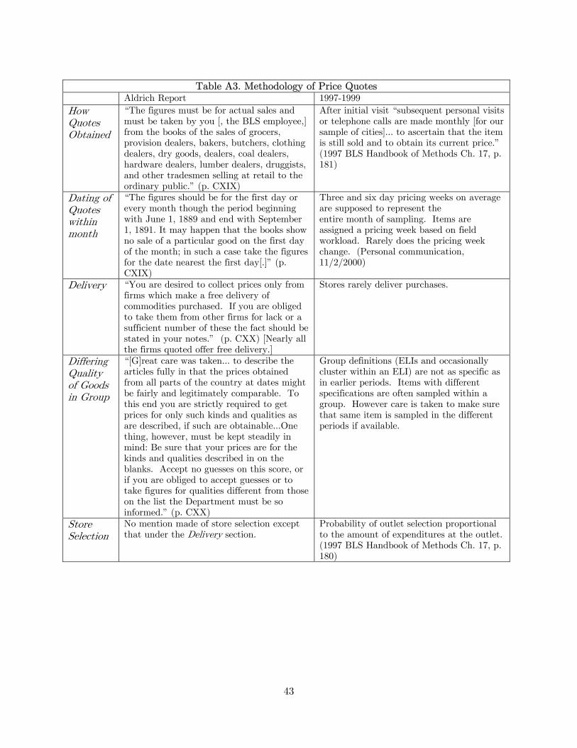
43
Table A3. Methodology of Price Quotes
Aldrich Report 1997-1999 How Quotes Obtained
“The figures must be for actual sales and must be taken by you [, the BLS employee,] from the books of the sales of grocers, provision dealers, bakers, butchers, clothing dealers, dry goods, dealers, coal dealers, hardware dealers, lumber dealers, druggists, and other tradesmen selling at retail to the ordinary public.” (p. CXIX)
After initial visit “subsequent personal visits or telephone calls are made monthly [for our sample of cities]... to ascertain that the item is still sold and to obtain its current price.” (1997 BLS Handbook of Methods Ch. 17, p. 181)
Dating of Quotes within month
“The figures should be for the first day or every month though the period beginning with June 1, 1889 and end with September 1, 1891. It may happen that the books show no sale of a particular good on the first day of the month; in such a case take the figures for the date nearest the first day[.]” (p. CXIX)
Three and six day pricing weeks on average are supposed to represent the entire month of sampling. Items are assigned a pricing week based on field workload. Rarely does the pricing week change. (Personal communication, 11/2/2000)
Delivery “You are desired to collect prices only from firms which make a free delivery of commodities purchased. If you are obliged to take them from other firms for lack or a sufficient number of these the fact should be stated in your notes.” (p. CXX) [Nearly all the firms quoted offer free delivery.]
Stores rarely deliver purchases.
Differing Quality of Goods in Group
“[G]reat care was taken... to describe the articles fully in that the prices obtained from all parts of the country at dates might be fairly and legitimately comparable. To this end you are strictly required to get prices for only such kinds and qualities as are described, if such are obtainable...One thing, however, must be kept steadily in mind: Be sure that your prices are for the kinds and qualities described in on the blanks. Accept no guesses on this score, or if you are obliged to accept guesses or to take figures for qualities different from those on the list the Department must be so informed.” (p. CXX)
Group definitions (ELIs and occasionally cluster within an ELI) are not as specific as in earlier periods. Items with different specifications are often sampled within a group. However care is taken to make sure that same item is sampled in the different periods if available.
Store Selection
No mention made of store selection except that under the Delivery section.
Probability of outlet selection proportional to the amount of expenditures at the outlet. (1997 BLS Handbook of Methods Ch. 17, p. 180)