Multi-Graph Tensor Networks

Yao Lei Xu, Kriton Konstantinidis, Danilo P. Mandic

Department of Electrical and Electronic EngineeringImperial College London

Multi-Graph Tensor Networks

Yao Lei Xu, Kriton Konstantinidis, Danilo P. Mandic

Department of Electrical and Electronic EngineeringImperial College London

Introduction

The multi-modal and irregular nature of modern big data is posing stern challenges totraditional learning systems, owing to the sheer volume, variety, veracity and velocityof modern data sources [1]. To this end, it is necessary to generalize deep learningapproaches to handle such irregular and multi-modal data.

Some of the most successful approaches for data analytics on irregular domains resortto graph signal processing techniques, because of their ability to provide insights intothe underlying data geometry [2]. When it comes to exceedingly large multi-modaldata, tensor-based methods have demonstrated their potential in effectively bypassingthe bottlenecks imposed by the curse of dimensionality in various learning tasks [1].

To provide a general framework that fully exploits the advantages of both graphs andtensors in a deep learning setting, we here generalize the RGTN concept in [3] to in-troduce the novel Multi-Graph Tensor Network (MGTN). In this way, the proposedMGTN is capable of handling irregular data residing on multiple graph domains, whilesimultaneously leveraging the compression properties of tensor networks to enhancemodelling power and reduce parameter complexity.

Fast Multi-Graph Tensor Network Model

Consider a multi-graph learning problem where the input is an order-(M + 1) ten-sor X ∈ RJ0×I1×I2×···×IM with J0 features indexed along M physical modes{I1, I2, . . . , IM}, such that a graph G(m) is associated with each of the Im modes,m = 1, . . . ,M . For this problem, we define:

1. A = {A(1),A(2), . . . ,A(M)}, a set of adjacency matrices A(m) ∈ RIm×Im con-

structed from the corresponding graphs G(m).

2. W = {W(1),W(2), . . . ,W(M)}, a set of weight matrices W(m) ∈ RJm×Jm−1

used for feature transforms, where Jm, for m = 1, . . . ,M controls the numberof feature maps at every m.

3. P = {P(1),P(2), . . . ,P(M)}, a set of propagation matrices P(m) ∈ RJm×Jm,

modelling the propagation of information over the neighbours of the graph G(m).

Using the above objects and an optional activation function, σ(·), we can now de-fine the general Multi-Graph Tensor Network (gMGTN) layer characterized by thefollowing forward pass:

Y = σ(F (M) ×1,M+1

3,4 W(M) ×12 · · · ×

12 F

(2) ×1,33,4 W

(2) ×12 F

(1) ×1,23,4 W

(1) ×12 X

)(1)

where F (m) = ten(I + (A(m) ⊗ P(m))). The so defined forward pass generates afeature map, Y ∈ RJM×I1×···×IM , from the input tensor, X , through a series ofmulti-linear graph filter and weight matrix contractions, which essentially iterates thegraph filtering operation across all M graph domains.

We can reduce the parameter complexity of gMGTN by: (i) approximating P(m) ≈ I

for m = 1, . . . ,M ; and (ii) using one single weight matrix, W(x) ∈ RJ1×J0, for allof the graph domains, where J1 controls the number of hidden units (feature maps).

This allows us to simplify the graph filter to F(m) = (I + A(m)), which leads to thefast Multi-Graph Tensor Network (fMGTN) forward pass:

Y = σ(F(M) ×M+1

2 · · · ×42 F

(2) ×32 F

(1) ×22 W

(1) ×12 X

)(2)

Model Architecture

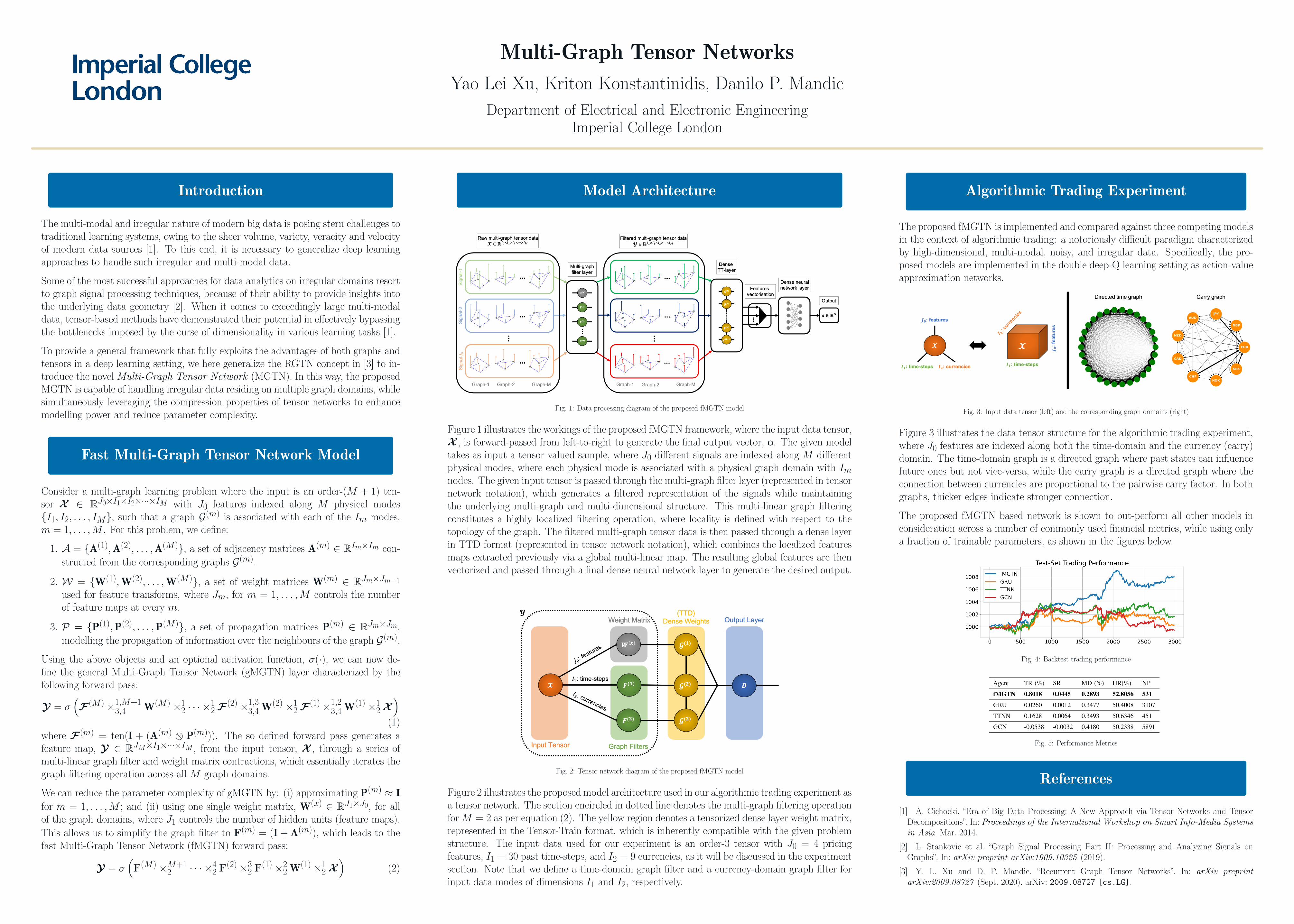
Fig. 1: Data processing diagram of the proposed fMGTN model

Figure 1 illustrates the workings of the proposed fMGTN framework, where the input data tensor,X , is forward-passed from left-to-right to generate the final output vector, o. The given modeltakes as input a tensor valued sample, where J0 different signals are indexed along M differentphysical modes, where each physical mode is associated with a physical graph domain with Imnodes. The given input tensor is passed through the multi-graph filter layer (represented in tensornetwork notation), which generates a filtered representation of the signals while maintainingthe underlying multi-graph and multi-dimensional structure. This multi-linear graph filteringconstitutes a highly localized filtering operation, where locality is defined with respect to thetopology of the graph. The filtered multi-graph tensor data is then passed through a dense layerin TTD format (represented in tensor network notation), which combines the localized featuresmaps extracted previously via a global multi-linear map. The resulting global features are thenvectorized and passed through a final dense neural network layer to generate the desired output.

Fig. 2: Tensor network diagram of the proposed fMGTN model

Figure 2 illustrates the proposed model architecture used in our algorithmic trading experiment asa tensor network. The section encircled in dotted line denotes the multi-graph filtering operationfor M = 2 as per equation (2). The yellow region denotes a tensorized dense layer weight matrix,represented in the Tensor-Train format, which is inherently compatible with the given problemstructure. The input data used for our experiment is an order-3 tensor with J0 = 4 pricingfeatures, I1 = 30 past time-steps, and I2 = 9 currencies, as it will be discussed in the experimentsection. Note that we define a time-domain graph filter and a currency-domain graph filter forinput data modes of dimensions I1 and I2, respectively.

Algorithmic Trading Experiment

The proposed fMGTN is implemented and compared against three competing modelsin the context of algorithmic trading: a notoriously difficult paradigm characterizedby high-dimensional, multi-modal, noisy, and irregular data. Specifically, the pro-posed models are implemented in the double deep-Q learning setting as action-valueapproximation networks.

Fig. 3: Input data tensor (left) and the corresponding graph domains (right)

Figure 3 illustrates the data tensor structure for the algorithmic trading experiment,where J0 features are indexed along both the time-domain and the currency (carry)domain. The time-domain graph is a directed graph where past states can influencefuture ones but not vice-versa, while the carry graph is a directed graph where theconnection between currencies are proportional to the pairwise carry factor. In bothgraphs, thicker edges indicate stronger connection.

The proposed fMGTN based network is shown to out-perform all other models inconsideration across a number of commonly used financial metrics, while using onlya fraction of trainable parameters, as shown in the figures below.

Fig. 4: Backtest trading performance

Fig. 5: Performance Metrics

References

[1] A. Cichocki. “Era of Big Data Processing: A New Approach via Tensor Networks and TensorDecompositions”. In: Proceedings of the International Workshop on Smart Info-Media Systemsin Asia. Mar. 2014.

[2] L. Stankovic et al. “Graph Signal Processing–Part II: Processing and Analyzing Signals onGraphs”. In: arXiv preprint arXiv:1909.10325 (2019).

[3] Y. L. Xu and D. P. Mandic. “Recurrent Graph Tensor Networks”. In: arXiv preprintarXiv:2009.08727 (Sept. 2020). arXiv: 2009.08727 [cs.LG].