yale university department of computer science · yale university department of computer science...

Yale UniversityDepartment of Computer Science

Calculi forFunctional Programming Languages

with Assignment

Daniel Eli Rabin

Research Report YALEU/DCS/RR-1107May 1996

ABSTRACTCalculi for

Functional Programming Languageswith Assignment

Daniel Eli Rabin1996

Pure functional programming and imperative programming appear to be contradictory approaches to the de-sign of programming languages. Pure functional programming insists that variables have unchanging bindingsand that these bindings may be substituted freely for occurrences of the variables. Imperative programming,however, relies for its computational power on the alteration of variable bindings by the action of the program.

One particular approach to merging the two design principles into the same programming language in-troduces a notion of assignable variable distinct from that of functionally bound variable. In this approach,functional programming languages are extended with new syntactic constructs denoting sequences of actions,including assignment to and reading from assignable variables. Swarup, Reddy and Ireland have proposed atyped lambda-calculus in this style as a foundation for programming-language design. Launchbury has pro-posed to extend strongly-typed purely functional programming in this style in such a way that assignments arecarried out lazily.

In this dissertationwe extend and correct the work of Odersky, Rabin, and Hudak givingan untyped lambda-calculus as a formalism for designing functional programming languages having assignable variables. Theextension encompasses two untyped calculi sharing a common core of syntactic constructs and rules corre-sponding to the similarities in all the typed proposals, and differing in ways that isolate the semantic differ-ences between those proposals. We prove the consistency and suitability for implementation of the two calculi.We adapt a technique of Launchbury and Peyton Jones to provide a safe type system for the calculi we study,thus providing a correct replacement for systems, now known to be flawed, originally proposed by Swarup,Reddy, Ireland, Chen, and Odersky.

Calculi forFunctional Programming Languages

with Assignment

A DissertationPresented to the Faculty of the Graduate School

ofYale University

in Candidacy for the Degree ofDoctor of Philosophy

byDaniel Eli Rabin

Dissertation Director: Professor Paul R.Hudak

May 1996

c Copyright by Daniel Eli Rabin 1996All Rights Reserved

To the memory of Richard Howard Trommer

CONTENTS

LIST OF FIGURES vii

LIST OF TABLES ix

ACKNOWLEDGMENTS xi

1 Introduction 11.1 The apparent incompatibility of assignment and substitution semantics : : : : : : : : : : : 21.2 Approaches from functional programming : : : : : : : : : : : : : : : : : : : : : : : : : : 3

1.2.1 State-transformer monads : : : : : : : : : : : : : : : : : : : : : : : : : : : : : : 31.2.2 The Imperative Lambda Calculus : : : : : : : : : : : : : : : : : : : : : : : : : : 51.2.3 The calculus λvar : : : : : : : : : : : : : : : : : : : : : : : : : : : : : : : : : : : 51.2.4 Lazy store transformers : : : : : : : : : : : : : : : : : : : : : : : : : : : : : : : 61.2.5 Common features : : : : : : : : : : : : : : : : : : : : : : : : : : : : : : : : : : 6

1.3 The Algol 60 heritage : : : : : : : : : : : : : : : : : : : : : : : : : : : : : : : : : : : : 71.4 Methodology : : : : : : : : : : : : : : : : : : : : : : : : : : : : : : : : : : : : : : : : : 81.5 Other related work : : : : : : : : : : : : : : : : : : : : : : : : : : : : : : : : : : : : : : 81.6 Overview of the dissertation : : : : : : : : : : : : : : : : : : : : : : : : : : : : : : : : : 9

2 Lambda-calculi with assignment 112.1 Mathematical preliminaries : : : : : : : : : : : : : : : : : : : : : : : : : : : : : : : : : 112.2 The basic applied lambda-calculus : : : : : : : : : : : : : : : : : : : : : : : : : : : : : : 142.3 Axiomatizing commands and assignment : : : : : : : : : : : : : : : : : : : : : : : : : : 162.4 Axioms for assignment : : : : : : : : : : : : : : : : : : : : : : : : : : : : : : : : : : : : 172.5 Locally defined store-variables : : : : : : : : : : : : : : : : : : : : : : : : : : : : : : : : 182.6 Purification: extracting the result of a store computation : : : : : : : : : : : : : : : : : : : 19

2.6.1 The general structure of purification rules : : : : : : : : : : : : : : : : : : : : : : 202.6.2 Eager versus lazy store-computations : : : : : : : : : : : : : : : : : : : : : : : : 212.6.3 Locally defined stores : : : : : : : : : : : : : : : : : : : : : : : : : : : : : : : : 22

2.7 Chapter summary : : : : : : : : : : : : : : : : : : : : : : : : : : : : : : : : : : : : : : 23

3 Proofs of the fundamental properties 273.1 A roadmap to the proofs in this chapter : : : : : : : : : : : : : : : : : : : : : : : : : : : 273.2 Basic concepts and techniques of reduction semantics : : : : : : : : : : : : : : : : : : : : 283.3 Factoring the notion of reduction : : : : : : : : : : : : : : : : : : : : : : : : : : : : : : : 29

3.3.1 The reduction relation!. : : : : : : : : : : : : : : : : : : : : : : : : : : : : : : 303.3.2 The modified computational reduction relation!! : : : : : : : : : : : : : : : : : 33

3.4 Keeping track of redexes : : : : : : : : : : : : : : : : : : : : : : : : : : : : : : : : : : : 343.4.1 Marked reductions : : : : : : : : : : : : : : : : : : : : : : : : : : : : : : : : : : 343.4.2 Interaction of!. with marked computational reduction : : : : : : : : : : : : : : : 35

3.5 Strong finiteness of developments modulo association : : : : : : : : : : : : : : : : : : : : 403.5.1 The weak Church-Rosser property : : : : : : : : : : : : : : : : : : : : : : : : : : 413.5.2 Finiteness of developments : : : : : : : : : : : : : : : : : : : : : : : : : : : : : 453.5.3 Strong finiteness of developments : : : : : : : : : : : : : : : : : : : : : : : : : : 47

3.6 The Church-Rosser property : : : : : : : : : : : : : : : : : : : : : : : : : : : : : : : : : 483.7 Standard evaluation order : : : : : : : : : : : : : : : : : : : : : : : : : : : : : : : : : : 483.8 Relating properties of!! to properties of! : : : : : : : : : : : : : : : : : : : : : : : : : 573.9 Chapter summary : : : : : : : : : : : : : : : : : : : : : : : : : : : : : : : : : : : : : : 59

v

vi

4 Operational equivalence 614.1 Definitions and basic results : : : : : : : : : : : : : : : : : : : : : : : : : : : : : : : : : 614.2 Some operational equivalences in λ[βδ!eag] and λ[βδ!laz] : : : : : : : : : : : : : : : : : : 624.3 Chapter summary : : : : : : : : : : : : : : : : : : : : : : : : : : : : : : : : : : : : : : 70

5 Simulation and conservation 715.1 Simulation of calculi with assignment by calculi with explicit stores : : : : : : : : : : : : : 71

5.1.1 The calculi with explicit stores : : : : : : : : : : : : : : : : : : : : : : : : : : : : 725.1.2 Equivalence of bubble/fuse rules and store-transition rules : : : : : : : : : : : : : 73

5.2 Calculi with assignments as conservative extensions of lambda-calculi : : : : : : : : : : : 825.2.1 Syntactic embedding : : : : : : : : : : : : : : : : : : : : : : : : : : : : : : : : : 835.2.2 The calculus λν : : : : : : : : : : : : : : : : : : : : : : : : : : : : : : : : : : : 845.2.3 Translating λ[βδσeag] into λν : : : : : : : : : : : : : : : : : : : : : : : : : : : : 855.2.4 Reversing the translation : : : : : : : : : : : : : : : : : : : : : : : : : : : : : : : 925.2.5 Establishing conservative extension : : : : : : : : : : : : : : : : : : : : : : : : : 955.2.6 Conservative extension for λ[βδ!laz] : : : : : : : : : : : : : : : : : : : : : : : : : 96

5.3 Chapter summary : : : : : : : : : : : : : : : : : : : : : : : : : : : : : : : : : : : : : : 96

6 Typed lambda-calculi with assignment 976.1 The Hindley/Milner polymorphic type system for functional languages : : : : : : : : : : : 976.2 What should a type system for a lambda-calculus with assignments do? : : : : : : : : : : : 1006.3 The Chen/Odersky type system for λ[βδ!eag] and λ[βδ!laz] : : : : : : : : : : : : : : : : : 1006.4 The type system LPJ for λ[βδ!eag] and λ[βδ!laz] : : : : : : : : : : : : : : : : : : : : : : 1046.5 The prospect for an untyped version of LPJ : : : : : : : : : : : : : : : : : : : : : : : : : 1166.6 Chapter summary : : : : : : : : : : : : : : : : : : : : : : : : : : : : : : : : : : : : : : 116

7 In conclusion 1177.1 Unfinished business : : : : : : : : : : : : : : : : : : : : : : : : : : : : : : : : : : : : : 1177.2 Future Work : : : : : : : : : : : : : : : : : : : : : : : : : : : : : : : : : : : : : : : : : 117

7.2.1 Mutable arrays and data structures : : : : : : : : : : : : : : : : : : : : : : : : : : 1177.2.2 Advanced control constructs : : : : : : : : : : : : : : : : : : : : : : : : : : : : : 118

7.3 Summary of technical results : : : : : : : : : : : : : : : : : : : : : : : : : : : : : : : : : 119

A Proofs of the fundamental properties for λ[βδσeag] and λ[βδσlaz] 121A.1 The reductions!. and!! : : : : : : : : : : : : : : : : : : : : : : : : : : : : : : : : : : 121A.2 Finite developments : : : : : : : : : : : : : : : : : : : : : : : : : : : : : : : : : : : : : 122A.3 The Church-Rosser property : : : : : : : : : : : : : : : : : : : : : : : : : : : : : : : : : 122A.4 Standardization : : : : : : : : : : : : : : : : : : : : : : : : : : : : : : : : : : : : : : : : 122A.5 Conclusion : : : : : : : : : : : : : : : : : : : : : : : : : : : : : : : : : : : : : : : : : : 125

B Changes in notation and terminology from previously published versions 127

BIBLIOGRAPHY 129

LIST OF FIGURES

1.1 The counter-object in monadic style : : : : : : : : : : : : : : : : : : : : : : : : : : : : : 5

2.1 Syntax of the pure untyped lambda-calculus λ[βδ]. : : : : : : : : : : : : : : : : : : : : : : 122.2 Syntax of the basic untyped lambda-calculus λ[βδ]. : : : : : : : : : : : : : : : : : : : : : 142.3 Reduction rules for the basic untyped lambda-calculus λ[βδ]. : : : : : : : : : : : : : : : : 142.4 Syntax of generic command constructs. : : : : : : : : : : : : : : : : : : : : : : : : : : : 162.5 Generic command reductions. : : : : : : : : : : : : : : : : : : : : : : : : : : : : : : : : 162.6 Syntax of basic assignment primitive commands. : : : : : : : : : : : : : : : : : : : : : : 172.7 Reduction rules for basic primitive store commands. : : : : : : : : : : : : : : : : : : : : : 172.8 Syntax for allocatable store-variables. : : : : : : : : : : : : : : : : : : : : : : : : : : : : 182.9 Reduction rules for allocatable store-variables. : : : : : : : : : : : : : : : : : : : : : : : : 192.10 Syntax of purification construct : : : : : : : : : : : : : : : : : : : : : : : : : : : : : : : 222.11 Syntax of purification contexts : : : : : : : : : : : : : : : : : : : : : : : : : : : : : : : : 222.12 Purification rules for λ[βδ!eag]. : : : : : : : : : : : : : : : : : : : : : : : : : : : : : : : 222.13 Purification rules for λ[βδ!laz]. : : : : : : : : : : : : : : : : : : : : : : : : : : : : : : : : 222.14 Syntax of λ[βδ!eag] and λ[βδ!laz] : : : : : : : : : : : : : : : : : : : : : : : : : : : : : : 242.15 Reduction rules common to both λ[βδ!eag] and λ[βδ!laz] : : : : : : : : : : : : : : : : : : 242.16 Syntax of purification contexts : : : : : : : : : : : : : : : : : : : : : : : : : : : : : : : : 242.17 Additional reduction rules for λ[βδ!eag] : : : : : : : : : : : : : : : : : : : : : : : : : : : 252.18 Additional reduction rules for λ[βδ!laz] : : : : : : : : : : : : : : : : : : : : : : : : : : : 25

3.1 Definition of the weight function. : : : : : : : : : : : : : : : : : : : : : : : : : : : : : : 463.2 Evaluation contexts for λ[βδ]. : : : : : : : : : : : : : : : : : : : : : : : : : : : : : : : : 483.3 Evaluation contexts for both λ[βδ!eag] and λ[βδ!laz] : : : : : : : : : : : : : : : : : : : : 483.4 Evaluation contexts for λ[βδ!eag] : : : : : : : : : : : : : : : : : : : : : : : : : : : : : : 483.5 Evaluation contexts for λ[βδ!laz] : : : : : : : : : : : : : : : : : : : : : : : : : : : : : : : 493.6 Subterm ordering for defining the leftmost redex : : : : : : : : : : : : : : : : : : : : : : : 49

5.1 Additional syntax for explicit-store calculi : : : : : : : : : : : : : : : : : : : : : : : : : : 715.2 Notation for explicit stores : : : : : : : : : : : : : : : : : : : : : : : : : : : : : : : : : : 725.3 Common reduction rules for explicit-store calculi : : : : : : : : : : : : : : : : : : : : : : 725.4 Reduction rules for eager explicit-store calculus λ[βδσeag] : : : : : : : : : : : : : : : : : 725.5 Reduction rules for lazy explicit-store calculus λ[βδσlaz] : : : : : : : : : : : : : : : : : : 725.6 The correspondence relation for terms : : : : : : : : : : : : : : : : : : : : : : : : : : : : 745.7 The correspondence relation for store-contexts and stores : : : : : : : : : : : : : : : : : : 745.8 Syntax of the local-name calculus λν : : : : : : : : : : : : : : : : : : : : : : : : : : : : 845.9 Reduction rules for the local-name calculus λν : : : : : : : : : : : : : : : : : : : : : : : 845.10 The implementation translation F for λ[βδσeag] : : : : : : : : : : : : : : : : : : : : : : : 865.11 Auxiliary function definitions for the translation F : : : : : : : : : : : : : : : : : : : : : 865.12 The inverse translation F1 from λν to λ[βδσeag] : : : : : : : : : : : : : : : : : : : : : : 93

6.1 Syntax of the let expression : : : : : : : : : : : : : : : : : : : : : : : : : : : : : : : : : 986.2 Reduction rule for let : : : : : : : : : : : : : : : : : : : : : : : : : : : : : : : : : : : : 986.3 Syntax of types for the Hindley/Milner polymorphic type system : : : : : : : : : : : : : : 986.4 Typing rules for the Hindley/Milner polymorphic type system : : : : : : : : : : : : : : : : 986.5 Structural rules for type derivations : : : : : : : : : : : : : : : : : : : : : : : : : : : : : 996.6 Syntax of types for Chen/Odersky type system for λ[βδ!eag] : : : : : : : : : : : : : : : : 1016.7 Chen/Odersky type system for λ[βδ!eag] : : : : : : : : : : : : : : : : : : : : : : : : : : : 1016.8 Syntax of types for LPJ : : : : : : : : : : : : : : : : : : : : : : : : : : : : : : : : : : : 1046.9 Type inference rules for LPJ : : : : : : : : : : : : : : : : : : : : : : : : : : : : : : : : : 1056.10 Syntax of types for LPJ : : : : : : : : : : : : : : : : : : : : : : : : : : : : : : : : : : : 106

vii

viii

6.11 Modified inference rule for LPJ : : : : : : : : : : : : : : : : : : : : : : : : : : : : : : 1066.12 Additional rules for LPJ : : : : : : : : : : : : : : : : : : : : : : : : : : : : : : : : : : 1066.13 Bound variables of a store-context : : : : : : : : : : : : : : : : : : : : : : : : : : : : : : 1086.14 The language Λok of non-stuck normal forms : : : : : : : : : : : : : : : : : : : : : : : : 113

7.1 Rule for control operator : : : : : : : : : : : : : : : : : : : : : : : : : : : : : : : : : : : 119

A.1 Evaluation contexts for λ[βδσeag] : : : : : : : : : : : : : : : : : : : : : : : : : : : : : : 123A.2 Evaluation contexts for λ[βδσlaz] : : : : : : : : : : : : : : : : : : : : : : : : : : : : : : 123A.3 Additional subterm ordering for λ[βδσeag] and λ[βδσlaz] : : : : : : : : : : : : : : : : : : 123

LIST OF TABLES

1.1 Contributions of the present dissertation to the design of functional programming languageswith assignment. : : : : : : : : : : : : : : : : : : : : : : : : : : : : : : : : : : : : : : : 2

ix

Acknowledgments

I began the research described in this dissertation in early 1992 in collaborationwith Martin Odersky and underthe supervision of Paul Hudak. Previous states of the work have been reported in the conference paper [Oder-sky et al., 1993] (also available as [Odersky et al., 1992]) and in more detail in the technical report [Oderskyand Rabin, 1993]. I have included material from these previous works as appropriate, correcting technicalerrors large and small, and revising the notation and exposition to fit the expanded scope of the dissertation.

It is safe to say that, without Martin’s enthusiasm for our interactive work and his tutelage in the often-frustrating craft of research, this dissertation could not possibly have come into existence. My supervisor, PaulHudak, acted as an unfailing cheerleader and collaborator during the intial years, and provided sound advice(which I sometimes ignored, to my sorrow).

Paul, Martin, and my other committee members, Young-il Choo, Mark P. Jones, and Uday S. Reddy, havebeen patient throughout the long process of finishing this dissertation. I thank them for the improvements thattheir comments and suggestions have brought about.

Paul Smolensky helped my decide to start graduate school, and John D. Corbett helped me enormously infinishing.

I gratefully acknowledge the financial assistance afforded by an IBM Graduate Fellowship during the aca-demic years 1992–94. My parents, William and Alice Rabin, provided the financial support necessary to finishthis work in 1994–96.

Palo Alto, CaliforniaApril 1996

xi

1Introduction

The design of certain functional programming languages (Haskell [Hudak et al., 1992] and Miranda [Turner,1985] among them) is renowned for its rejection of assignment to variables as a basis for specifying com-putations. This rejection stems both from the desire to free the programmer from low-level implementationconcerns and from the urge to provide a simple, powerful theory of program transformation. To its proponents,the avoidance of variable assignment earns for these languages the taxonomic designation of pure functionalprogramming languages.

The absence of variable assignment, however, mitigates the usefulness of pure functional programminglanguages in at least two ways. First, although the freedom from the need to express low-level implementa-tion concerns has great force in speeding the prototypingof programs, this force has a dark side in the inabilityto control these details for engineering purposes. This concern recapitulates the lingeringmistrust of compilerson the part of assembly-language programmers, the difference being that functional-programming compilertechnology has not (yet) attained the triumphal level of object-code efficiency that characterizes many of to-day’s conventional-language compilers.

A second factor mitigating the virtue of purity is that many programming problems are about changingstate. The rise in popularity of object-oriented programming (stemming ultimately from the design of Sim-ula [Birtwistle et al., 1973]) attests to the usefulness of a programming paradigm in which program objectsencapsulating local states simulate the behavior of the real-world objects that are the subject of the computerprogram. It is possible for programs written in pure functional programming languages to simulate statefulcomputations by means of transition functions operating on an explicitly-represented state. However, it isdifficult for such a functional program to represent its use of state as simply as programs in a conventionallanguage in which the state is implicit and ever-present.

In the last few years there have been several proposals for introducingassignment into pure functional pro-gramming languages without compromising their essential susceptibility to formal reasoning. Although theseproposals differ in detail, an identifiable subset of them revolves around a common set of design principles:we add to the syntax of the pure functional programming language a distinct set of terms for representing com-mands, the command terms are constrained to be meaningful only when chained together in a linear sequence,and observations of the store are expressed as commands, not values. These principles, properly implemented,are sufficient to preserve referential transparency in the extended language.

The published proposals are variously presented as untyped or typed lambda-calculi, or informally pre-sented as extensions to functional programming languages. In this dissertation we bring a unity of approachto several of these proposals. We use the techniques of untyped lambda-calculi to develop an untyped oper-ational semantics for pure functional programming with assignment. We give extended lambda-calculi thatmodel two variants of our target class of programming-language proposals; we prove fundamental propertiesof these calculi, and we introduce a type system that excludes programs having run-time failures owing tomisuse of the store constructs.

The most immediate antecedent of the current work is the work of Swarup, Reddy, and Ireland on the Im-perative Lambda Calculus (ILC) [Swarup et al., 1991; Swarup, 1992]. This work is presented formally usingboth operational and denotational techniques, but it is essentially a typed system. In contrast, we follow ourprevious work on λvar [Odersky et al., 1993; Odersky and Rabin, 1993] in adopting the operational-semanticstechniques of untyped lambda-calculus as our formal basis; this approach allows us to study computational is-sues and type-safety issues separately. We further exercise our approach by extending it to cover the proposalof Launchbury [Launchbury, 1993] that store transformations should be executed on demand just as functionalcomputations are in non-strict functional programming languages; our extension represents the first fully for-mal basis we know of for Launchbury’s proposal.

In addition to bringing contrasting techniques to bear on these existing proposals, the present dissertationalso presents some corrections to previous work. We cite our own mistakes first: the proof of the Church-Rosser and standardization properties in [Odersky and Rabin, 1993] contains a subtle flaw that we correcthere in an interesting way. In addition, we modify the calculi presented in our earlier work to allow a more

1

2

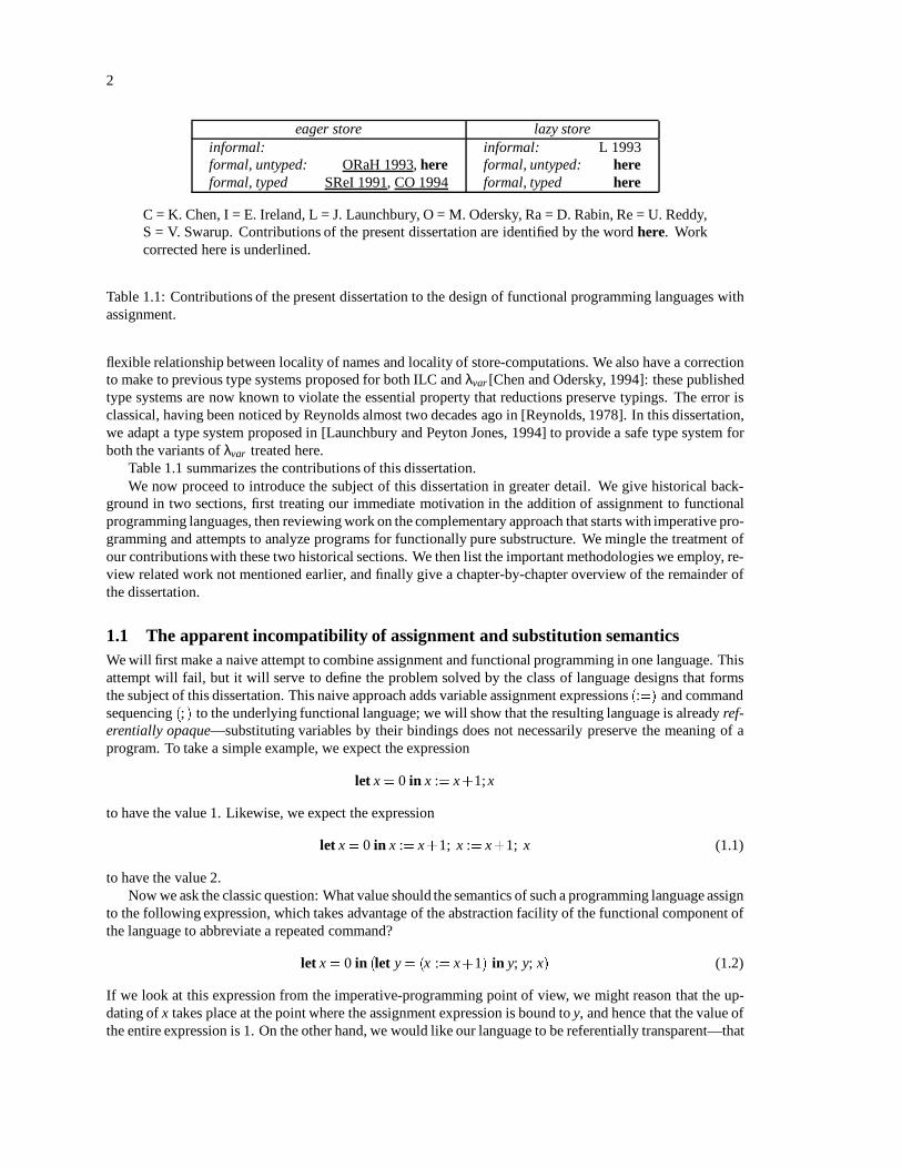
eager store lazy storeinformal:formal, untyped: ORaH 1993, hereformal, typed SReI 1991, CO 1994

informal: L 1993formal, untyped: hereformal, typed here

C = K. Chen, I = E. Ireland, L = J. Launchbury, O = M. Odersky, Ra = D. Rabin, Re = U. Reddy,S = V. Swarup. Contributions of the present dissertation are identified by the word here. Workcorrected here is underlined.

Table 1.1: Contributions of the present dissertation to the design of functional programming languages withassignment.

flexible relationship between locality of names and locality of store-computations. We also have a correctionto make to previous type systems proposed for both ILC and λvar [Chen and Odersky, 1994]: these publishedtype systems are now known to violate the essential property that reductions preserve typings. The error isclassical, having been noticed by Reynolds almost two decades ago in [Reynolds, 1978]. In this dissertation,we adapt a type system proposed in [Launchbury and Peyton Jones, 1994] to provide a safe type system forboth the variants of λvar treated here.

Table 1.1 summarizes the contributions of this dissertation.We now proceed to introduce the subject of this dissertation in greater detail. We give historical back-

ground in two sections, first treating our immediate motivation in the addition of assignment to functionalprogramming languages, then reviewing work on the complementary approach that starts with imperative pro-gramming and attempts to analyze programs for functionally pure substructure. We mingle the treatment ofour contributions with these two historical sections. We then list the important methodologies we employ, re-view related work not mentioned earlier, and finally give a chapter-by-chapter overview of the remainder ofthe dissertation.

1.1 The apparent incompatibility of assignment and substitution semanticsWe will first make a naive attempt to combine assignment and functional programming in one language. Thisattempt will fail, but it will serve to define the problem solved by the class of language designs that formsthe subject of this dissertation. This naive approach adds variable assignment expressions (:=) and commandsequencing (; ) to the underlying functional language; we will show that the resulting language is already ref-erentially opaque—substituting variables by their bindings does not necessarily preserve the meaning of aprogram. To take a simple example, we expect the expression

let x = 0 in x := x+1; x

to have the value 1. Likewise, we expect the expression

let x = 0 in x := x+1; x := x+1; x (1.1)

to have the value 2.Now we ask the classic question: What value should the semantics of such a programming language assign

to the following expression, which takes advantage of the abstraction facility of the functional component ofthe language to abbreviate a repeated command?

let x = 0 in (let y = (x := x+1) in y; y; x) (1.2)

If we look at this expression from the imperative-programming point of view, we might reason that the up-dating of x takes place at the point where the assignment expression is bound to y, and hence that the value ofthe entire expression is 1. On the other hand, we would like our language to be referentially transparent—that

3

is, it ought to be valid to substitute x := x+1 for y to obtain (1.1) again, which has the value 2. We now havea conflict: two perfectly reasonable, but different, ways of evaluating this small program yield different an-swers. 1 If we had given the semantics of this language via a formal calculus, we would say that the calculusis non-confluent or lacks the Church-Rosser property. Informally, we can just state that the semantics of thelanguage is inconsistent with the semantics of function application defined by substitution (which is what wegenerally mean by referential transparency).

This conflict lies at the heart of the divergent evolution of functional and imperative languages. If we banimperative constructs, we can have both referential transparency and confluence (this is the Church-Rossertheorem of classical lambda-calculus [Barendregt, 1984]), but if we insist on retaining assignment we appearto lose both. It is thus an important question whether this conflict can be resolved

The answer is that it can. Just as imperative constructs supply a suitable villain for the functional pointof view, so also the underspecified order of evaluation provides a villain for the imperative point of view. Ifa formal calculus requires that evaluation of a program takes place in a certain order, consistency can be re-established. This is exactly what a denotational semantics for an imperative language does. It is even possibleto carry out this approach for a higher-order language, especially if the language uses the call-by-value evalua-tion order, in which argument expressions are always evaluated before the function applications of which theyare part. Scheme [Clinger and Rees, 1991] and Standard ML [Milner et al., 1990] are two examples of lan-guages designed in this fashion. These languages, however, are outside the scope of this dissertation becausethey are not referentially transparent, even with respect to the call-by-value β-rule used in [Plotkin, 1975].

1.2 Approaches from functional programmingSection 1.1 depicts a dichotomous choice in programming-language design: it seems we can obtain either fullreferential transparency, or have assignment in the language, but not both. Recent research approaching theissue from the point of view of functional programming, however, has shown this dichotomy to be only anapparent one. We now give an overview of this line of research, whose foundations in the lambda-calculusare the subject of this dissertation. We treat the complementary approach, from the point of view of Algol-likelanguages, in Section 1.3.

The point of attack for all the proposals we survey here is against the tacit assumption in Section 1.1 that,because a notion of assignable store requires a sequencing of commands, this order of evaluation must some-how be derived from the evaluation order already present in the functional language. If sequences of com-mands affecting the store were somehow disentangled from expressions denoting values, the example (1.2)given above would become meaningless, since that example contains assignment commands in a position inwhich a pure functional language would require a value expression.

1.2.1 State-transformer monads

One of the first proposals along these lines was Wadler’s proposal [Wadler, 1990a; Wadler, 1992a] to take in-spiration from the theoretical work of Moggi [Moggi, 1989; Moggi, 1991] and adopt the category-theoreticnotion of monad as a program-construction framework within functional programming languages. For thepurposes of the present informal exposition, a monad on some underlying domain consists of a type construc-tor that takes any type to a type of “generalized commands” that yield that type. There is an operator . forsequencing such generalized commands and an operator " for embedding values as trivial generalized com-mands. These operators are required to obey algebraic laws similar (but not identical) to the unit and associa-tive laws of a monoid.

The symbols . and " that we have just introduced for the monad operators are the same symbols that weuse in the body of the dissertation (starting in Section 2.3) for syntactic constructs with a monad-like inter-pretation. We adopt these symbols here for consistency. Although we treat them informally as functions in a

1A situation like this almost occurs in the programming language Standard ML, which is defined by a precise semantics in [Milneret al., 1990]. That semantics specifies the interpretation of (1.2) yielding the answer 1 by way of specifying the order in which evaluationtakes place.

4

programming language, the syntax we later give them as part of formal calculi differs in some respects.2

The monad structure is more general than we require—we are only concerned with monads of state trans-formers. As given by Moggi and Wadler, such a monad has its operator and unit element defined (using in-formal functional-programming notation in the style of Haskell) by

type ST α = S! Sα (1.3)

. : ST α! (α! ST β)! ST β (1.4)

f .g = λs:let hs0;xi = f s in g x s0; (1.5)

" : α! ST α (1.6)

"x = λs:hs;xi (1.7)

where the type S represents the type of the store (which will always be invisible to user programs), and s, s0

are variables having this type.This monad would not be interesting if only these generic operators were available. In order to model the

creation, update, and reading of assignable variables, we make use of the additional operators

new : α! ST (Ref α) (1.8)

update : Ref α! α! ST () (1.9)

read : Ref α! ST α; (1.10)

where Ref α is the type of references to values of another type α.The operator new accepts a value of type α and returns a state-transformer that creates and returns a new

reference to that value in the store. The operator update returns a state-transformer that carries out a newassignment to an existence reference to a value of type α, and the operator read returns a state-transformer forobserving the value referred to by a given reference.

These additional operations can be defined in terms of an implementation of the store, but we do not yetrequire this level of detail. The main point is that the types associated with the store operators enforces therestriction that the commands they denote only have their imperative meaning when placed in a linear sequenceusing .. It is the imposition of this linear sequence on the accesses to the store that insulates the order of accessto the store from the evaluation order of expressions in the language.

In this dissertation we always notate the operator . as including the bound variable of the function definingits second argument. We also make . right-associative: M.x(N .y P) and M.xN .y P mean the same thing.On the other hand, (M. x N) .y P is a syntactically distinct expression which is related to the others by theanalogue of the associative law for command sequences.

The approach via monads deals with the example (1.2) by distinguishing between commands as state-transformers and their effects. Thus the meaning of (1.2), as re-expressed in terms of state-transformers, isunambiguously 2: the variable y is bound to the state-transformer itself, and the process of carrying out thisbinding merely constructs the state-transformer without carrying out its effect. The state-transformation isthen carried out twice owing to the occurrences of y in a command-sequence context.

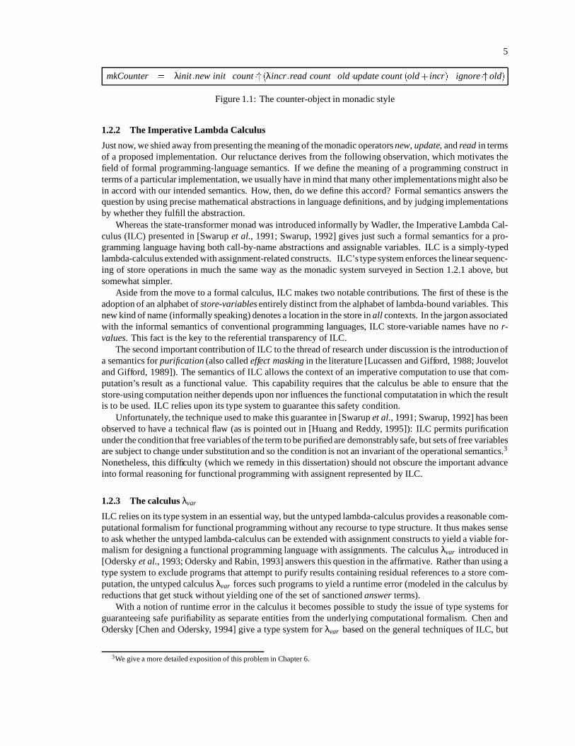
Figure 1.1 gives an example of a program in a pure functional programming language extended with anassignment monad. The example function makeCounter accepts an initial value (an integer) and initializes acounter variable, returning an object (implemented as a function) that produces a store-transformer for incre-menting the count.

Hudak’s proposal for mutable abstract data types [Hudak, 1992] is similar to the use of state-transformermonads but less general in intent and somewhat simpler algebraically. Hudak focuses on the relationship be-tween direct-style and continuation-style functional expressions of the mutation of data structures, and on thealgebraic construction of accessors and constructors in the two styles for given data types.

2The untyped nature of the calculi introduced in this dissertation requires us to incorporate the functional nature of the second operandof . into the syntax of the operator itself by means of a binding occurrence of a variable. The operator thus always appears in the formM .x N in the formal chapters of this dissertation.

5

mkCounter = λinit:new init.count " (λincr:read count.old update count (old + incr). ignore" old)

Figure 1.1: The counter-object in monadic style

1.2.2 The Imperative Lambda Calculus

Just now, we shied away from presenting the meaning of the monadic operators new, update, and read in termsof a proposed implementation. Our reluctance derives from the following observation, which motivates thefield of formal programming-language semantics. If we define the meaning of a programming construct interms of a particular implementation, we usually have in mind that many other implementations might also bein accord with our intended semantics. How, then, do we define this accord? Formal semantics answers thequestion by using precise mathematical abstractions in language definitions, and by judging implementationsby whether they fulfill the abstraction.

Whereas the state-transformer monad was introduced informally by Wadler, the Imperative Lambda Cal-culus (ILC) presented in [Swarup et al., 1991; Swarup, 1992] gives just such a formal semantics for a pro-gramming language having both call-by-name abstractions and assignable variables. ILC is a simply-typedlambda-calculus extended with assignment-related constructs. ILC’s type system enforces the linear sequenc-ing of store operations in much the same way as the monadic system surveyed in Section 1.2.1 above, butsomewhat simpler.

Aside from the move to a formal calculus, ILC makes two notable contributions. The first of these is theadoption of an alphabet of store-variables entirely distinct from the alphabet of lambda-bound variables. Thisnew kind of name (informally speaking) denotes a location in the store in all contexts. In the jargon associatedwith the informal semantics of conventional programming languages, ILC store-variable names have no r-values. This fact is the key to the referential transparency of ILC.

The second important contribution of ILC to the thread of research under discussion is the introduction ofa semantics for purification (also called effect masking in the literature [Lucassen and Gifford, 1988; Jouvelotand Gifford, 1989]). The semantics of ILC allows the context of an imperative computation to use that com-putation’s result as a functional value. This capability requires that the calculus be able to ensure that thestore-using computation neither depends upon nor influences the functional computatation in which the resultis to be used. ILC relies upon its type system to guarantee this safety condition.

Unfortunately, the technique used to make this guarantee in [Swarup et al., 1991; Swarup, 1992] has beenobserved to have a technical flaw (as is pointed out in [Huang and Reddy, 1995]): ILC permits purificationunder the condition that free variables of the term to be purified are demonstrably safe, but sets of free variablesare subject to change under substitution and so the condition is not an invariant of the operational semantics.3

Nonetheless, this difficulty (which we remedy in this dissertation) should not obscure the important advanceinto formal reasoning for functional programming with assignent represented by ILC.

1.2.3 The calculus λvar

ILC relies on its type system in an essential way, but the untyped lambda-calculus provides a reasonable com-putational formalism for functional programming without any recourse to type structure. It thus makes senseto ask whether the untyped lambda-calculus can be extended with assignment constructs to yield a viable for-malism for designing a functional programming language with assignments. The calculus λvar introduced in[Odersky et al., 1993; Odersky and Rabin, 1993] answers this question in the affirmative. Rather than using atype system to exclude programs that attempt to purify results containing residual references to a store com-putation, the untyped calculus λvar forces such programs to yield a runtime error (modeled in the calculus byreductions that get stuck without yielding one of the set of sanctioned answer terms).

With a notion of runtime error in the calculus it becomes possible to study the issue of type systems forguaranteeing safe purifiability as separate entities from the underlying computational formalism. Chen andOdersky [Chen and Odersky, 1994] give a type system for λvar based on the general techniques of ILC, but

3We give a more detailed exposition of this problem in Chapter 6.

6

this type system suffers from the same subtle flaw as ILC; the type system we present in Chapter 6 remediesthis flaw.

The results of our previous work on λvar are incorporated into this dissertation, but the calculus itself is re-named λ[βδ!eag] in the uniform nomenclature introduced here. We also take the opportunity to correct severalflaws in the application of proof techniques of the pure lambda-calculus to proving the fundamental propertiesof λvar ; the details are treated in Chapter 3. We also extend the formalism of λvar to account for the variantlanguage discussed in the next subsection.

1.2.4 Lazy store transformers

All the work on lazy functional programming with assignment that we have cited so far makes a tacit assump-tion that the command sublanguage behaves like commands in a conventional imperative language: com-mands are executed in order as soon as they are encountered. Launchbury, however, observes in [Launch-bury, 1993] that this semantics for command sequences is not the only one possible. The evaluation sequenceof a functional language can be lazy or eager (yielding semantically distinct languages); command sequencesare subject to a similar choice. Pure lazy functional programs can be understood as carrying out computa-tion to produce a value only in response to a demand for that value; likewise, Launchbury proposes commandsequences that are only executed as far as necessary to produce the results that are demanded. Launchburyclaims that the resulting style of imperative programming meshes more easily with an ambient lazy functionalprogramming language, and he gives examples to support this claim.

In order to see the distinction introduced by Launchbury, we consider a very short program written in thenotation of the calculi we introduce in the formal chapters of this dissertation. In this notation, the constructpure marks off a command sequence whose final result is to be returned as a value to the surrounding func-tional program; the result term itself is marked by the operator " applied to the final expression in the commandsequence. Our example program is

pure(loop; "3) (1.11)

where loop is some command whose execution never ends (we will see later that such terms exist). In a moreconventional functional programming language, this example might be notated

newstore ( loop;return3):

The result returned by the imperative computation in (1.11) in fact does not depend on that computation. Nev-ertheless, in ILC and λvar the execution of the program would result in the non-terminating execution of loop.In Launchbury’s proposal, however, the program yields the value 3, since no demand is ever made for anycomponent of the introduced store. This extra laziness enters quite naturally if one approaches the design ofimperative-functional programming languages directly at the level of extending an existing lazy functionallanguage (as is done for example in [Peyton Jones and Wadler, 1993]). In such an approach, it actually takessome extra work to specify that the state-transformers ought to be strict.

The informalityof the original presentation of the lazy store-transformer proposal leads us to inquire whetherthe λvar formalism can be adapted to a different order of command execution. We have carried out this adapta-tion, and the resulting change in formalism is so minor that the two resulting calculi (λ[βδ!eag] and λ[βδ!laz])can be presented in parallel throughout the dissertation with only occasional remarks where the differences aretreated. The most significant departure from this parallel structure is reported in Section 5.2.6: a proof tech-nique based on continuation-passing-style translations is not easily transferred from λ[βδ!eag] to λ[βδ!laz].

1.2.5 Common features

We have seen in this section that a whole family of related proposals for pure functional programming withassignment has arisen. The common features of these proposals are:

Substitutable(lambda-bound)variables and store-variables are distinct syntactic entities. Store-variablesmay be a distinct kind of value called a reference.

7

Commands form a distinct subcategory of expressions. Commands can only be composed in a linearsequence

Access to the current value of a store-variable or reference is accomplished by a special command, notby the use of an expression having a value.

In addition to these features that are common to all of the proposals presented so far, usefulness for pro-gramming requires that there be a way of coercing a command into an expression that denotes a value. Thiscoercion must fail if there are dangling references to the command’s store or if the command makes referenceto another store. ILC and λvar devote explicit, formal attention to this issue; the informal language-based pro-posals generally concentrate the concern on an opaque primitive function called newstore or run that carriesout the coercion.

In Chapter 2 we will represent these common features in the design of the two lambda-calculi λ[βδ!eag]and λ[βδ!laz]. These two calculi reflect these common features in the bulk of their specifications and differonly in their treatment of execution order within command sequences.

1.3 The Algol 60 heritageThe preceding discussion in Section 1.2 recounts the immediate motivation of the present work in the searchfor a harmonious introduction of assignment constructs into referentially-transparent functional programminglanguages. This combination of paradigms, however, may also be approached from the imperative-program-ming point of view, and indeed it has been, dating from the days of the great progenitor, Algol 60 [Nauret al., 1960; Naur et al., 1963]. It is a peculiarity of Algol 60, little imitated in its successors, that its de-fault parameter-passing mechanism is call-by-name: procedure invocation is defined by the copy rule statingthat the procedure invocation has exactly the same meaning as the defining text of the procedure, but withall occurrences of the formal parameter being replaced by the actual parameter supplied to the procedure (asan expression of the language). Of course, the definition requires the renaming of bound variables to avoidclashes, but this requirement easily becomes second nature—the real semantics is in the idea of textual re-placement. The copy rule, which is exactly the β-rule of the lambda calculus [Church, 1951] may reasonablybe claimed to capture the notion of referential transparency which will be characteristic of the language-designproposals we consider in this dissertation.

Algol 60 with call-by-name parameter passing is, in fact, referentially transparent. The semantic ambigu-ity demonstrated in (1.2) above cannot occur because commands themselves cannot be bound to variables inAlgol 60—they can only be abstracted via the procedure-definition mechanism. It is possible to define a proce-dure whose body is the command whose duplication would cause problems, but the definition itself cannot bemistaken for a context in which the incrementing of x should take place. Only in the context of a command se-quence is a command defined. This property of Algol 60 is the germ of the common feature of the approachessurveyed in Section 1.2 that separates commands and expressions syntactically, and gives commands theirmeaning only in the right context. This orthogonality of functional and imperative features of Algol 60 hasbeen refined into a more modern language design by Reynolds in his design of Forsythe [Reynolds, 1988],and it has been studied formally in [Weeks and Felleisen, 1992; Weeks and Felleisen, 1993].

The importance for us of considering the Algol 60 tradition is that it has given rise to a significant alterna-tive approach to the melding of functional and assignment-based programming. Reynolds [Reynolds, 1978]proposed a way of controlling the interference of assignment-based subcomputations within Algol-like pro-grams by means of a syntactic analysis. This concern is analogous to our concern with purification in ourfunctional languages with assignment. Reynolds’s proposal, however, has a more symmetrical structure thanour language: whereas we distinguish between the inside and outside of a scope of store usage, Reynoldsaddresses the possibility of mutual interference between (possibly) parallel subexpressions of a program.

The paper [Reynolds, 1978] is also interesting to us because it contains an early exposition of the prob-lem that spoils the type systems given in [Swarup et al., 1991] and [Chen and Odersky, 1994]. The problemwas later rectified in the context of Algol-like languages by Reynolds himself by use of intersection types[Reynolds, 1989] and more recently by O’Hearn, Power, Takeyama, and Tennent [O’Hearn et al., 1995] witha type system (SCIR) loosely based on linear logic [Girard, 1987]. This latter type system has been adapted to

8

a revised language based on ILC by Huang and Reddy [Huang and Reddy, 1995]. The type system we presentin Chapter 6 is an alternative that more closely follows the original outlines of ILC, although the SCIR-basedapproach may prove to be more generally applicable.

1.4 MethodologyWe have claimed the formalization of several language proposals as a key contribution of this dissertation.We use two main formalisms. First, and most pervasively, we follow [Plotkin, 1975] and model the basic(untyped) computational meaning of programs in each language in terms of an extended lambda-calculus en-dowed with a reduction relation that models computation. We also use the apparatus of type theory, especiallyof polymorphic type systems [Girard, 1990; Reynolds, 1974; Milner, 1978], in proving the desirable proper-ties of the proposed type systems with respect to their underlying untyped calculi.

The lambda-calculus serves both as the operational semantics of computation in our programming lan-guages and also as the basis for formal reasoning about these programs. In order to form the basis for a func-tional language with assignment, a calculus must have several key properties:

Church-Rosser property. The result of a computation must be independent of the order in which reduc-tions are carried out. This property guarantees that terms have a single meaning: the reduction systemprovides a semantics for the language.

Standard reduction order. There is a deterministic reduction order that always reduces a term to an an-swer if the term can be reduced to such a normal form. This property makes plausible the claim that thecalculus serves as the basis for designing a programming language: it is possible to write a deterministicprogram to carry out the evaluation. Aside from its implications for automation, standardization sim-plifies some proofs (such as that of Lemma 5.1.6 in the present dissertation, for example) by allowingthe consideration of only a single reduction sequence.

Simulationby store-based machine. There is a faithful simulation of evaluation in the calculus by a cal-culus that manipulates an explicit store in a single-threaded fashion. This property validates the claimthat the imperative features of a calculus can actually be simulated by the imperative features of a ma-chine.

The lambda-calculus methodology requires some change in the usual vocabulary of discussion concerningpurification. It is common, in discussing the problem of masking effects in a functional/imperative language,to phrase the central problem in terms of implementation: will the language prevent access to a store locationafter its thread dies? Can different evaluation orders give different results? In terms of a lambda-calculus,these questions resolve to one question: is the calculus Church-Rosser? If it is, then certainly evaluation or-der can make no difference in outcome. Furthermore, if we understand a dangling-location reference as astuck evaluation in the calculus, we see that the Church-Rosser property guarantees that the problem is in theprogram, not in the choice of evaluation strategy.

The presentation in Chapter 6 uses the standard apparatus of type theory: type systems are given as infer-ence systems, with type derivations as proof trees in the inference system so defined.

1.5 Other related workWe have already surveyed the most closely related literature in the preceding sections. We now survey workthat stands outside of our narrowly-defined topic but is related either by attacking similar problems or by useof similar methodology.

The oldest approach to introducing imperative constructs into functional languages is to express the stateas an explicit object that is passed around by the program. This is the approach taken by most denotationalsemantics for imperative languages (see, for example, [Stoy, 1977] or [Schmidt, 1986]). When applied tofunctional programming, this approach relies on an analysis carried out by the language processor to achieveefficient execution: it must be determined that the use of the state object is actually single-threaded and thusthat it is safe to implement state mutations via in-place update of data structures. Schmidt [Schmidt, 1985]

9

and Fradet [Fradet, 1991] give syntactic criteria for proving single-threadedness; Guzman [Guzman and Hu-dak, 1990; Guzman, 1993] gives a type system in which well-typed programs possessing certain designatedtypes are thereby proved to be single-threaded; another approach based on abstract interpretation is presentedin [Odersky, 1991]. Wadler has investigated the use of type systems based on linear logic for this purpose[Wadler, 1990b; Wadler, 1991]; several other researchers have also investigated the use of linear logic as adesign principal in functional programming languages [Lafont, 1988; Wakeling and Runciman, 1991; Reddy,1991; Reddy, 1993].

Riecke, along with Viswanathan, [Riecke, 1993; Riecke and Viswanathan, 1995] has approached the con-struction of a safe type system for roughly the class of languages inhabited by our calculi, but their methodol-ogy makes essential use of properties of denotational models and is inherently based on types. Furthermore,the language treated is call-by-value (whereas our calculi are call-by-name). These contrasts to our work placeRiecke and Viswanathan’s approach in a distinct thread of research.

Not all related research deals directly with the issue of state in pure functional programming: there is asubstantial body of work influenced by the designs of Lisp and Scheme. The work of Felleisen, Friedman, andcolleagues into the foundations of Scheme-like languages [Felleisen, 1987; Felleisen and Friedman, 1987a;Felleisen and Friedman, 1987b; Felleisen and Hieb, 1992] uses extended lambda-calculi to provide semanticsfor such languages. Despite the fact that this work deals exclusively with call-by-value languages and doesnot insist on preserving the reasoning properties of the pure fragment (such as the validity of the call-by-nameβ-rule), we have adopted much of its methodology in the present work. In a similar vein, Mason and Talcotthave investigated the formal semantics of much the same class of programming languages in works such as[Mason, 1986; Mason and Talcott, 1991; Mason and Talcott, 1992a; Mason and Talcott, 1992b].

A recent paper by Sato [Sato, 1994], which is very much in the vein of the work by Mason and Talcott,presents a Scheme-like calculus in which syntactic criteria for the placment of update commands provide ref-erential transparency. Sato’s division of reductions into sequential and parallel reductions is reminiscent ofthe present work’s segregation of expressions and commands, but it is not clear whether there is any formalcorrespondence.

Graham and Kock [Graham and Kock, 1991] present a design for a functional language with assignment.Their design rests on static syntactic detection of opportunities for violation of referential transparency, andthey report a formal proof of the desired properties. The language, however, appears not to have higher-orderfunctions, and their syntactic restrictions appear less natural than those for our typed languages; furthermore,the correctness of purification is only proved for a subset of the language.

Further removed from our work on assignment, but still related, is a stream of research on devising con-structs for input/output in pure functional programming languages. Input/output shares with assignment theneed to institute a sequencing structure for commands: devices used include continuations and streams [Hu-dak and Sundaresh, 1988] and monads [Wadler, 1992b; Peyton Jones and Wadler, 1993]. Gordon’s thesis onthe subject [Gordon, 1994] contains a detailed survey of this research. Input/output differs from assignment,however, in its need to represent an activity that is external to the program and not necessarily under its control.Issues of reactivity and synchronization thus arise that have no counterpart in the study of assignment.

1.6 Overview of the dissertationThe contents of this dissertation are organized as follows.

Chapter 2 defines the calculi λ[βδ!eag] and λ[βδ!laz] that are studied in rest of the dissertation. The calculiare introduced feature-by-feature both informally in terms of the intended meaning and as formal systems.

The next three chapters, which develop the theory of the untyped calculi in detail, form the core of the the-sis. Chapter 3 gives the proofs of the Church-Rosser and standardization theorems for both calculi. Chapter 4explores the operational-equivalence theory (the intended principles of program equivalence) of the calculi.In Chapter 5 we look at the relationship of λ[βδ!eag] and λ[βδ!laz] to other calculi. In the first part of Chap-ter 5, we introduce the calculi λ[βδσeag] and λ[βδσlaz] which have explicit stores in the language syntax.The equivalence in operational semantics between these calculi and their forbears substantiates the claim thatthe latter really axiomatize the use of astore. In the second part of Chapter 5, we prove the important factthat λ[βδ!eag] forms a conservative extension of a calculus representing a purely functional programminglanguage; we conjecture that the result also holds for λ[βδ!laz].

10

Chapter 6 complements the completely untyped treatment of the preceding chapters with a presentation ofa safe type system for the calculi λ[βδ!eag] and λ[βδ!laz]. This type system is an adaptation of a type systemproposed by Launchbury and Peyton Jones [Launchbury and Peyton Jones, 1994]; we prove its safety andremark on the prospect for use of the unadapted type system.

Chapter 7 summarizes the dissertation and suggests further work in the area.

2Lambda-calculi with assignment

In this chapter we introduce the extended lambda-calculi that form the subject matter of this dissertation. Aftera brief section that provides for later reference some of the basic mathematical tools we employ in describingthe calculi, we build up a description of our calculi with assignment starting from the pure lambda-calculus andadding features incrementally. We concentrate here on motivating and describing the design of these calculi;we leave the mathematical treatment of their properties for the following chapters.

The two calculi we introduce, which correspond to the columns in Table 1.1 on page 2, have almost iden-tical structures: they differ only in one rule. We will thus be able to describe the two calculi in parallel for thegreater part of this dissertation, and will treat their differences as the exception rather than the rule.

Our starting point will be the pure lambda-calculus (Section 2.1), which is a pure calculus of functions.Finding this setting too austere to model even the common practice of modern purely functional program-ming languages, we add primitive functions and data constructors to form the calculus λ[βδ] (Section 2.2).With λ[βδ] as a point of departure we first add constructs to model sequences of commands. After introducingthose command constructs that make sense irrespective of the domain of commands envisioned (Section 2.3),we specialize our attention to stores and assignments by introducing (and axiomatizing) some primitive com-mands in Section 2.4.

At this point the heart of the matter may seem to be addressed, but there are two important further re-finements to be dealt with. First, we address the axiomatization of locally-defined store-variables in Sec-tion 2.5, and second we introduce locally-defined stores in Section 2.6.1. In respect of our approach to oursubject matter from the functional-programming side, we use the term purification to denote the introduc-tion of boundaries beyond which a local store is both ineffective and unobservable. It is only in the ruleswe devise for the treatment of locally-defined stores that the difference between the notion of eager and lazystore-transformations emerges into the design of these calculi.

2.1 Mathematical preliminariesOur presentation of our lambda-calculi with assignment rests on a large body of well-developed mathematicalformalisms. We make particular use of proof techniques from the pure lambda-calculus, for which our mainreference is [Barendregt, 1984]. We engage, however, in significant extensions to the pure lambda-calculus;we collect some of the mathematical terms we use for these extensions in the present section.

Languages of terms and reductions

A formal calculus consists of a set of terms, called a language, and rules for manipulating the terms. We usethe terminology of lambda-calculus in calling these reduction rules and the relation between terms that theydefine reduction. We call a subterm that matches the left-hand side of a rule a redex and the result of rewritingit a reduct. When a term is rewritten according to a reduction rule, any portion of a designated subterm thatsurvives into the rewritten term is called a residual of that subterm.

Languages are defined inductively by rules giving basic terms and productions for forming terms fromsimpler terms. We often have occasion to define a language based on the inductive description of anotherlanguage. For example, we describe the incremental additionof features to the calculi presented in this chapterby incorporating all the productions of a previously-described language. A further example of this techniqueis the formation from a language of a language of contexts by adjoining a special term [] (the “hole”) to thelanguage as a production for the top-level syntactic category of terms; we usually intend to admit only thoseterms so formed that have exactly one occurrence of the hole.

The language of lambda-calculus

The language of the pure lambda-calculus itself is defined by the productions in Figure 2.1. The pure lambda-calculus contains only variables, abstractions of terms, and applications of one term to another. Although

11

12

x;y 2 VariablesM;N 2 Terms

M ::= x variablesj λx:M abstractionsj MN applications

Figure 2.1: Syntax of the pure untyped lambda-calculus λ[βδ].

the standard notation for application is simple juxtaposition, we deviate from this standard throughout thisdissertation because we will have occasion to annotate the application operator, and it is difficult to annotatea blank. We retain the usual lambda-calculus convention that application () associates the left.

The sole reduction rule of the pure lambda-calculus, β, makes use of the notion of substitutionand is givenin Figure 2.3.

Bound variables

The abstraction construct λx:M is said to bind the variable x, that is, occurrences of x within M but not withinany distinct occurrence of λx: are considered to have a unique identity separate from all other variables. Thismeaning is underscored by considering terms of the lambda-calculus to be distinct only up to the equivalenceof α-renaming, which permits the renaming the bound variable of an abstraction as long as all the bound oc-currences are renamed accordingly. The α-renaming equivalence allows the very convenient α-renaming con-vention, which is that we always pick an exemplar of an equivalence class of terms under α-renaming suchthat all bound and free variables have distinct names. This convention saves us considerable effort in writingexplicit renamings of bound variables whenever we discuss reductions that move terms into the scope of abound name.

An occurrence of a variable that is not bound is called free; we denote the set of free variables of a termM by fv M. A term M is called closed if fv M is the empty set.

In the course of this dissertation, we will have occasion to introduce new variable-bindingconstructs. Suchconstructs will be subject to the same conventions whether the issue is mentioned or not.

Extended lambda-calculi

We can extend the pure lambda-calculus by introducing term-constructors and reduction rules. Although weseldom use the following terminology, it is convenient for the current discussion to call attention to three pos-sible kinds of syntactic extension:

Names. An extension may introduce new syntactic categories of names, distinct from the variables ofpure lambda-calculus.

Binding constructs. As discussed in Section 2.1, constructs may be introduced to delimit scopes forparticular names. Each such construct comes with a notion of α-equivalence.

Free constructors. These are term-constructors that are neither names nor binders of names.

The pure lambda-calculus itself has one term-constructor of each type, application () being the sole free con-structor.

An extended calculus may introduce new binding constructs for an existing syntactic category of names.

Substitution

A fundamental operation on terms is substitutionof a term for all occurrences of a free variable in another term.Substitution forms the foundation of the operational semantics of the lambda-calculus, but it can actually bedefined wherever names are used. The notion of substitution is defined along with the notion of free variable,

13

which in turn embodies the basic notion of a name-binding construct: the bound name is distinct from anyname present in an outer scope.

Definition 2.1.1 (Substitution) For terms M, N, and variable x in some extended lambda-calculus, the sub-stitution of M for x in N, denoted [M=x]N, is a term defined inductively by the rules

[M=x] x M

[M=x] y y (x 6 y)

[M=x] (λy:N) λy:[M=x]N

[M=x] (N1 N2) ([M=x]N1) ([M=x]N2 )

[M=x] T(N1 ;: : : ;Nn) T ([M=x]N1 ;: : : ;[M=x]Nn)

where T denotes any free syntactic constructor of the extended language, and n denotes its arity.

Definition 2.1.1 makes essential use of the α-renaming convention in the rule for substituting into an ab-straction: the convention permits us to avoid mention of a case in which the variable bound by the abstractionhas the same name as the variable for which we are substituting. We merely assume that α-renaming hassolved the problem for us before the definition of substitution is invoked.

An important elementary property of sequenced substitutions is the following lemma on interchanging theorder of two substitutions. This lemma finds use in establishing the confluence of lambda-calculi.

Lemma 2.1.2 (Substitution) For terms M1, M2, N and variables x;y such that x 6 y and x 62 fv M2, we have

[M2=y] [M1=x]N [[M2=y]M1=x] [M2=y]N:

Proof: By induction on the structure of N.Base cases:

N x.

[M2=y] [M1=x] x [M2=y]M1; likewise, [[M2=y]M1=x] [M2=y] x [[M2=y]M1=x] x [M2=y]M1.

N y.

[M2=y] [M1=x] y [M2=y] yM2; likewise, [[M2=y]M1=x] [M2=y] y [[M2=y]M1=x]M2M2, since x 62fv M2.

Induction steps:

N λz:N0 .

In this case, [M2=y] [M1=x] (λz:N0 ) [M2=y] (λz:[M1=x]N0 ) λz:[M2=y] [M1=x]N0 . By the inductionhypothesis, this last expression is equivalent to λz:[[M2=y] M1=x] [M2=y]N0 . Applying the definition ofsubstitution in reverse establishes the statement of the lemma in this case.

The statement of the lemma follows for all other constructed terms by essentially the same argument.

This concludes the proof of Lemma 2.1.2.

Normal form

A term in a lambda-calculus to which no reduction rule applies is said to be in normal form.

14

x;y 2 VariablesM;N 2 Terms

cn 2 Constructors of arity nf 2 Primitive functionsA 2 Answers

M ::= x variablesj cn constructorsj f primitivesj λx:M abstractionsj MN applications

A ::= fj cn A1 Ak; k n

let x = M in N (λx:N) M convenient abbreviation

Figure 2.2: Syntax of the basic untyped lambda-calculus λ[βδ].

(λx:M) N ! [N=x]M (β)f M ! δ( f ;M) (δ)

δ( f ; (λx:M)) = Nf (λx:M)δ( f ; f1) = Nf ; f1 f1

δ( f ;cn M1 Mn) = Nf ;cn M1 Mn

Figure 2.3: Reduction rules for the basic untyped lambda-calculus λ[βδ].

2.2 The basic applied lambda-calculusSince we are using lambda-calculi to model the extension of pure functional programming, we first give thecalculus with which we model pure functional programming itself. Although it is possible to use the purelambda-calculus for this purpose, we find it more plausible to acknowledge the existence of primitive valuesand operations in all existing functional languages. Furthermore, the constructions given in Chapter 5 makeessential use of this feature. This consideration leads us to extend the pure lambda-calculus with constructorsand primitive function symbols (Figure 2.2). Constants are represented in this calculus as constructors of arityzero. Since we will need to distinguish among the several calculi to be discussed in this dissertation, we in-troduce a systematic naming convention for calculi: the character λ is followed by a bracketed list identifyingthe features of the calculus. The basic calculus presented in this section is denoted λ[βδ].

The reduction rules that enable λ[βδ] to model the computations of functional programming are given inFigure 2.3. The rule β is exactly as in the pure lambda-calculus: it models parameter passing by term sub-stitution. Rule δ gives the computational model for primitive functions. The apparent complexity of the rulestems from the need to limit the power of such terms, since it is well known (see [Barendregt, 1984]) that in thepresence of arbitrary δ-rules a calculus might fail to be confluent (a property defined in Section 3.2 below).The actual rule given is weak enough to avoid this pitfall. Essentially, it says that a primitive f is definedby lambda-terms giving its meaning when applied to a λ-abstraction and when applied to constructed values.Such definitions cannot examine the deeper structure of the argument to f . We will see in Chapter 3 that thisrestriction permits λ[βδ] to be confluent.

As an example of how primitive functions are represented in λ[βδ], consider the operator + on integers.The integers themselves are represented by nullary constructors, one for each integer. The operation+ is thendescribed by a countable (and obviously recursive) collection of rules such as +1!+1 , where +1 is itselfa primitive function with defining rules such as +1 0! 1 and +1 5! 6.

15

The terms Nf , Nf ; f1 , and Nf ;cn that appear in the definition of the auxiliary function δ(—;—) in Figure 2.3are the degrees of freedom we have in our restricted δ-rules. For each primitive function f defined in a particu-lar instance of λ[βδ] we may define Nf , specifying the behavior of f on arguments that are lambda-abstractions,one term Nf ; f1 specifying how f acts on each primitive function f1 , and one term Nf ;cn for each constructor cn

specifying how f acts on values constructed by cn. We need not give all these terms: it is permitted for a prim-itive function to be partial. For example, the addition function would not be defined on any constructors thatare not numerals. This careful structuring of δ-rule definitions restricts the power of such rules to detection ofone layer of syntactic structure of value-terms, branching to one of several lambda-definable computations.As we mentioned above, this restriction is sufficient to ensure that our calculi can be confluent in the presenceof δ-rules.

We curry our definition of primitives for two main reasons. First (and less important), we obtain the usualnotational advantage of currying, in that we do not need to introduce any special notation for multiple-argumentprimitives. More importantly, we will be proving theorems about the existence of deterministic standard or-ders of evaluation for all our calculi of concern. For such a theorem to be true, a calculus must commit to theevaluation order for arguments to a primitive function in order to break the symmetry of syntax that an uncur-ried representation offers. The curried formulation is a convenient way of allowing the standard evaluationorder to arise naturally.1

We can also define booleans by designating particular nullary constructors true and false; we can thusdefine if by Nif ;true λx:λy:x and Nif ;false λx:λy:y . However, in the case of if it is just as easy to use theChurch-encoded truth values λx:λy:x and λx:λy:y directly.2

The rule δ only applies when the argument expression is a constructed value, a primitive function, or anabstraction: this restriction is built into the definition of the auxiliary function δ(—;—). We can exploit thisfact to simulate the behavior of call-by-value languages by defining a primitive function force, setting Nforce

λx:x. We can also define a function strict as λf :λx: f (force x). These definitions work because they requirethe argument to force to be a value before the application expression is reduced.

The usual technique used to simulate call-by-value parameter passing is to modify the rule β. This mod-ification (introduced in [Plotkin, 1975]) involves a division of expressions into applications and all other ex-pressions, which are now termed values. The modified rule βV has the same rewriting effect as the originalrule β, but only applies when the argument expression is a value. This restriction reflects the notion that onlyan evaluated expression is substituted into the body of the function in a call-by-value language.

We mention the contrast between call-by-name and call-by-value calculi at this point because we will haveoccasion later in this chapter to introduce a similar contrast between lazy and eager store-computations. Just asthe rules β and βV differ only in the syntactic form of the argument terms, so also the rules defining purificationsof lazy and eager store-computations will differ only in the syntactic form of the contexts from which thepurification rule extracts a pure result.

The operational semantics we use throughout our treatment distinguishes a certain subset of terms as an-swers A, the observable results of terminating computations. There may be normal forms that are not answers:such terms are regarded as indicating a run-time error. For a basic example of such a term, consider the term

+ true1;

where + is a primitive implementing addition on integers (themselves represented as nullary constructors).The definition of the primitive + contains no defining case for the constructor true, so this term cannot bereduced. However, it is not an answer because+ is a primitive, not a constructor of arity 2 or higher as requiredby the definition when applied to two terms as is the case here. This particular example of a “stuck” term (anadjective we will continue to use) has an obvious correspondence to a type error in a programming language.

1The operator == for store-variable identity introduced in Section 2.5 is subject to the same issues as primitive-function definitions.2Church encoding [Church, 1951] represents various mathematical constructs as lambda-terms by giving those constructs interpreta-

tions as higher-order functions. Each natural number, for example, is identified with a term that iterates an unknown function that numberof times on an unknown argument. The encoding at hand, that for truth values, is based on the idea of conditionals picking one of twoarguments. The encoding for true picks the first; that for false picks the second.

16

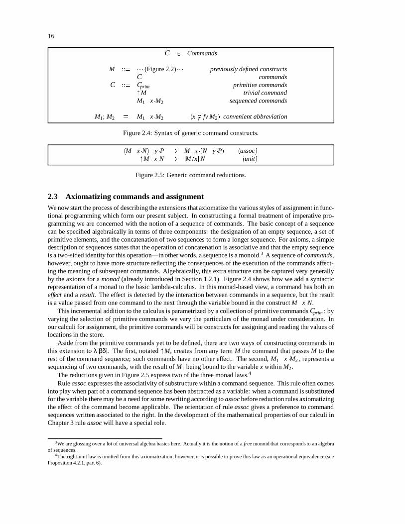
C 2 Commands

M ::= (Figure 2.2) previously defined constructsj C commands

C ::= Cprim primitive commandsj "M trivial commandj M1 .x M2 sequenced commands

M1; M2 M1 .x M2 (x 62 fv M2) convenient abbreviation

Figure 2.4: Syntax of generic command constructs.

(M. x N) .y P ! M.x (N .y P) (assoc)"M.x N ! [M=x]N (unit)

Figure 2.5: Generic command reductions.

2.3 Axiomatizing commands and assignmentWe now start the process of describing the extensions that axiomatize the various styles of assignment in func-tional programming which form our present subject. In constructing a formal treatment of imperative pro-gramming we are concerned with the notion of a sequence of commands. The basic concept of a sequencecan be specified algebraically in terms of three components: the designation of an empty sequence, a set ofprimitive elements, and the concatenation of two sequences to form a longer sequence. For axioms, a simpledescription of sequences states that the operation of concatenation is associative and that the empty sequenceis a two-sided identity for this operation—in other words, a sequence is a monoid.3 A sequence of commands,however, ought to have more structure reflecting the consequences of the execution of the commands affect-ing the meaning of subsequent commands. Algebraically, this extra structure can be captured very generallyby the axioms for a monad (already introduced in Section 1.2.1). Figure 2.4 shows how we add a syntacticrepresentation of a monad to the basic lambda-calculus. In this monad-based view, a command has both aneffect and a result. The effect is detected by the interaction between commands in a sequence, but the resultis a value passed from one command to the next through the variable bound in the construct M.x N.

This incremental addition to the calculus is parametrized by a collection of primitive commands Cprim : byvarying the selection of primitive commands we vary the particulars of the monad under consideration. Inour calculi for assignment, the primitive commands will be constructs for assigning and reading the values oflocations in the store.

Aside from the primitive commands yet to be defined, there are two ways of constructing commands inthis extension to λ[βδ]. The first, notated "M, creates from any term M the command that passes M to therest of the command sequence; such commands have no other effect. The second, M1 .x M2 , represents asequencing of two commands, with the result of M1 being bound to the variable x within M2.

The reductions given in Figure 2.5 express two of the three monad laws.4

Rule assoc expresses the associativity of substructure within a command sequence. This rule often comesinto play when part of a command sequence has been abstracted as a variable: when a command is substitutedfor the variable there may be a need for some rewriting according to assoc before reduction rules axiomatizingthe effect of the command become applicable. The orientation of rule assoc gives a preference to commandsequences written associated to the right. In the development of the mathematical properties of our calculi inChapter 3 rule assoc will have a special role.

3We are glossing over a lot of universal algebra basics here. Actually it is the notion of a free monoid that corresponds to an algebraof sequences.

4The right-unit law is omitted from this axiomatization; however, it is possible to prove this law as an operational equivalence (seeProposition 4.2.1, part 6).

17

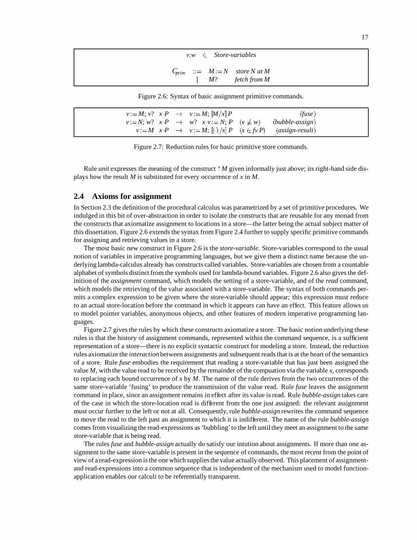
v;w 2 Store-variables

Cprim ::= M :=N store N at Mj M? fetch from M

Figure 2.6: Syntax of basic assignment primitive commands.

v :=M; v?.x P ! v :=M; [M=x]P (fuse)v :=N; w?.x P ! w?.x v := N; P (v 6 w) (bubble-assign)

v :=M.x P ! v :=M; [( )=x] P (x 2 fv P) (assign-result)

Figure 2.7: Reduction rules for basic primitive store commands.

Rule unit expresses the meaning of the construct "M given informally just above; its right-hand side dis-plays how the result M is substituted for every occurrence of x in M.

2.4 Axioms for assignmentIn Section 2.3 the definition of the procedural calculus was parametrized by a set of primitive procedures. Weindulged in this bit of over-abstraction in order to isolate the constructs that are reusable for any monad fromthe constructs that axiomatize assignment to locations in a store—the latter being the actual subject matter ofthis dissertation. Figure 2.6 extends the syntax from Figure 2.4 further to supply specific primitive commandsfor assigning and retrieving values in a store.

The most basic new construct in Figure 2.6 is the store-variable. Store-variables correspond to the usualnotion of variables in imperative programming languages, but we give them a distinct name because the un-derlying lambda-calculus already has constructs called variables. Store-variables are chosen from a countablealphabet of symbols distinct from the symbols used for lambda-bound variables. Figure 2.6 also gives the def-inition of the assignment command, which models the setting of a store-variable, and of the read command,which models the retrieving of the value associated with a store-variable. The syntax of both commands per-mits a complex expression to be given where the store-variable should appear; this expression must reduceto an actual store-location before the command in which it appears can have an effect. This feature allows usto model pointer variables, anonymous objects, and other features of modern imperative programming lan-guages.

Figure 2.7 gives the rules by which these constructs axiomatize a store. The basic notion underlying theserules is that the history of assignment commands, represented within the command sequence, is a sufficientrepresentation of a store—there is no explicit syntactic construct for modeling a store. Instead, the reductionrules axiomatize the interaction between assignments and subsequent reads that is at the heart of the semanticsof a store. Rule fuse embodies the requirement that reading a store-variable that has just been assigned thevalue M, with the value read to be received by the remainder of the compuation via the variable x, correspondsto replacing each bound occurrence of x by M. The name of the rule derives from the two occurrences of thesame store-variable ‘fusing’ to produce the transmission of the value read. Rule fuse leaves the assignmentcommand in place, since an assignment remains in effect after its value is read. Rule bubble-assign takes careof the case in which the store-location read is different from the one just assigned: the relevant assignmentmust occur further to the left or not at all. Consequently, rule bubble-assign rewrites the command sequenceto move the read to the left past an assignment to which it is indifferent. The name of the rule bubble-assigncomes from visualizing the read-expressions as ‘bubbling’ to the left until they meet an assignment to the samestore-variable that is being read.

The rules fuse and bubble-assign actually do satisfy our intution about assignments. If more than one as-signment to the same store-variable is present in the sequence of commands, the most recent from the point ofview of a read-expression is the one which supplies the value actually observed. This placement of assignment-and read-expressions into a common sequence that is independent of the mechanism used to model function-application enables our calculi to be referentially transparent.

18

v;w 2 store-variable

Cprim ::= (Figure 2.6) previously-defined commandsj νv:M introduce new store-variablej v== w test store-variable identity

Figure 2.8: Syntax for allocatable store-variables.

The precision required of a formal system demands that we provide the additional rule assign-result tocover the case in which the remainder of a command sequence observes not just the effect of an assignmentcommand, but also its functional result. To see why this is necessary, note that the left-hand side of the rulefuse is given in terms of the syntactic abbreviation ‘;’ defined in Figure 2.4. Expanding the abbreviation givesthe new left-hand side v :=M .z v? .x P; where z is a variable that does not occur free in v?.x P (which isto say that it does not occur free in P). Thus fuse does not apply in the case in which z does occur free in P,and hence we must supply a rule to cover this case if we want the calculus to reflect the intended semantics forassignment. Rule assign-result does this job by supplying a neutral value as the functional value of the assign-ment command wherever this value happens to be observed in the sequel. In the remainder of this dissertationwe denote this neutral value, which is an instance of a nullary constructor c0 (constant) by ().5

The definition of assign-result is somewhat arbitrary, in that the rule is specified to apply only when thestore-variable v has become known. It is certainly possible to consider a variant rule

N :=M.x P!N :=M; [( )=x]P; (x 2 fv P)

which does not force the computation of the store-variable. It is easier, however, to define evaluation contexts(Chapter 3) uniformly if we require computation to seek an actual store-variable as target of an assignmentcommand regardless of the context in which the assignment command appears.

There are some notable differences between the notion of assignable store introduced here and the con-structs available in most popular imperative programming languages. First, there is no restriction on the valuesthat may be assigned to a store-variable: any expression in the language is eligible, even other store-variables.Second, the name of a store-variable v does not denote its ‘current value’—there is no such concept. Instead,the name v merely denotes itself, and there is an associated command v? for finding the most-recently-assignedvalue for v and transmitting it to subsequent commands via term-substitution. Lastly, there is no analogue inour calculi to the distinctionbetween variables and pointers present in several popular conventional languages.In conventional languages both a variable itself and a pointer to the variable denote the variable’s storage, butin different ways according to context. As l-values, both a variable and its pointer denote the location, but asr-values, the variable denotes the contents whereas the pointer denotes the location. As just mentioned, ther-value interpretation is absent in our calculi.6

2.5 Locally defined store-variablesSo far, our formalism has nothing to say about where store-variables come from—we are given all the store-variables that will ever exist at the outset. In programming terms, they are all global variables. This simplifi-cation results from a deliberate decision to present the basic formalism for assignment in as much isolation aspossible. However, no reasonable account of imperative programming can neglect the notion of store-variablescope, by which the programmer may introduce a store-variable that is known (within the scope of its decla-ration) to be distinct from all other store-variables in the program. We now rectify this omission.

We do so by augmenting the basic store formalism given in Section 2.4 with constructs that allow theallocation of new variables in the store. Figure 2.8 introduces two new syntactic constructs. The expression

5By ‘neutrality’ we mean here that () is distinct from any other constant having an intended meaning, such as constants representingnumbers.

6The class of “conventional languages” here includes Algol 60, C, Pascal and Scheme but excludes Algol 68, Forsythe, and StandardML.

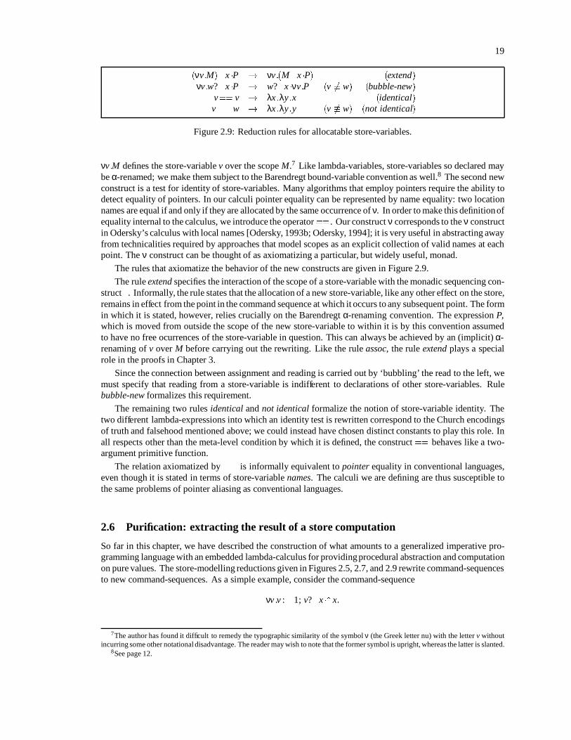
19

(νv:M) .x P ! νv:(M. x P) (extend)νv:w? .x P ! w?.x νv:P (v 6 w) (bubble-new)

v== v ! λx:λy:x (identical)v== w ! λx:λy:y (v 6 w) (not identical)

Figure 2.9: Reduction rules for allocatable store-variables.

νv:M defines the store-variable v over the scope M.7 Like lambda-variables, store-variables so declared maybe α-renamed; we make them subject to the Barendregt bound-variable convention as well.8 The second newconstruct is a test for identity of store-variables. Many algorithms that employ pointers require the ability todetect equality of pointers. In our calculi pointer equality can be represented by name equality: two locationnames are equal if and only if they are allocated by the same occurrence of ν. In order to make this definitionofequality internal to the calculus, we introduce the operator ==. Our construct ν corresponds to the ν constructin Odersky’s calculus with local names [Odersky, 1993b; Odersky, 1994]; it is very useful in abstracting awayfrom technicalities required by approaches that model scopes as an explicit collection of valid names at eachpoint. The ν construct can be thought of as axiomatizing a particular, but widely useful, monad.

The rules that axiomatize the behavior of the new constructs are given in Figure 2.9.

The rule extend specifies the interaction of the scope of a store-variable with the monadic sequencing con-struct .. Informally, the rule states that the allocation of a new store-variable, like any other effect on the store,remains in effect from the point in the command sequence at which it occurs to any subsequent point. The formin which it is stated, however, relies crucially on the Barendregt α-renaming convention. The expression P,which is moved from outside the scope of the new store-variable to within it is by this convention assumedto have no free ocurrences of the store-variable in question. This can always be achieved by an (implicit) α-renaming of v over M before carrying out the rewriting. Like the rule assoc, the rule extend plays a specialrole in the proofs in Chapter 3.

Since the connection between assignment and reading is carried out by ‘bubbling’ the read to the left, wemust specify that reading from a store-variable is indifferent to declarations of other store-variables. Rulebubble-new formalizes this requirement.

The remaining two rules identical and not identical formalize the notion of store-variable identity. Thetwo different lambda-expressions into which an identity test is rewritten correspond to the Church encodingsof truth and falsehood mentioned above; we could instead have chosen distinct constants to play this role. Inall respects other than the meta-level condition by which it is defined, the construct == behaves like a two-argument primitive function.

The relation axiomatized by == is informally equivalent to pointer equality in conventional languages,even though it is stated in terms of store-variable names. The calculi we are defining are thus susceptible tothe same problems of pointer aliasing as conventional languages.

2.6 Purification: extracting the result of a store computation

So far in this chapter, we have described the construction of what amounts to a generalized imperative pro-gramming language with an embedded lambda-calculus for providingprocedural abstraction and computationon pure values. The store-modelling reductions given in Figures 2.5, 2.7, and 2.9 rewrite command-sequencesto new command-sequences. As a simple example, consider the command-sequence

νv:v := 1; v?.x " x:

7The author has found it difficult to remedy the typographic similarity of the symbol ν (the Greek letter nu) with the letter v withoutincurring some other notational disadvantage. The reader may wish to note that the former symbol is upright, whereas the latter is slanted.

8See page 12.

20

It should be obvious that this little program returns the result 1; indeed we have the sequence of reductions

νv:v := 1; v?.x " x ! νv:v := 1; [1=x] (" x) (by fuse) νv:v := 1; "1:

This is a normal form; no further reductions are possible. However, this term is not the same as the answer-term 1, no matter how obvious it may be that this is its meaning. We have no rules for extracting the answer1 from the residue of the store-computation.

It might be tempting to supply a rule that strips away the context νv:v := 1; []; however, there is dangerhere. Suppose that we had started with the only-slightly-different initial term

νw:νv:v := w; v? .x " x

yielding the only-slightly-different sequence of reductions

νw:νv:v := w; v? .x " x ! νw:νv:v := w; [w=x] (" x) (by fuse) νw:νv:v := w; "w:

What happens if we just strip away the command-sequence context in the same way as before? Unfortunately,we would obtain the free store-variable w, which was bound before. In informal implementational terms, thiswould correspond to allowing the store-variable w to outlive its scope and become a dangling pointer; in formalterms we cannot hope to have a consistent calculus if bound names can escape their bonds.

We refer to the problem raised by these examples as the need for a purification construct in designs forfunctional languages with assignment. The escape of bound store-variables must clearly be prohibited by anyreasonable proposal for a purification construct, but name-escape is not the only issue involved: we will alsohave to consider the effect of purification constructs on the informal interpretationof store-variables as storagelocations. As will further emerge, purification constructs are the place where we distinguish between eagerand lazy uses of stores.

2.6.1 The general structure of purification rules

The problem of purification divides into two independent questions.

When in a store-computation do result values become available, and

What result values are legal?

These two questions are reflected in the general structure of purification rules that we present in this sub-section. Purification rules divide the store-computation to be purified into a store context and a result expres-sion. The question of when results become available arises because the result of a store-computation may notdepend on the entire computation. For example, suppose we are given the initial term

νv:v := 1; v?.x " 2:

The result 2 does not depend on the assignment v :=1. It is thus reasonable to try to write purification rules thatallow this result to be extracted from the store-computation context even though that context contains a latentassignment and a dependent read. The issue becomes more dramatic if we replace the innocuous assignmentv :=1 with some term Ω having no normal form to give the fragment

νv:Ω; v? .x " 2:

An eager-store calculus with assignment will compute forever trying to find what command is present, whereasa lazy-store calculus with assignment can return 2 immediately.

The question of what terms are considered legal to purify is considerably more complicated, and admitsa spectrum of answers. We have already seen two extreme points on this spectrum: a locally-allocated store-variable should never be extracted from its surrounding store-computation, whereas it is always safe to do

21

so with a constant (nullary constructor). With more complex result expressions, which may mix constantswith unevaluated expressions, the question of purification must be deferred until it is possible to see whichof the simple cases applies. The process of purification must therefore consider the following cases for resultexpressions:

1. Some subexpressions (such as store-variables) can be recognized to spoil purity merely by their syntac-tic form;

2. some (such as constants) can be recognized to be purifiable merely by their syntactic form;

3. some (such as variables or applications) must have any judgment as to their purifiability deferred untilfurther computation has taken place; and finally,

4. the purity of constructed expressions depends on the purity of their subexpressions.

In terms of our informal understanding of the problem this can only be correct if the result expressionM is free of any remaining reference to the state represented by the store context S[], since such a referencewill be nonsensical once the representation of that state is erased from the program. Furthermore, it mustbe impossible for an expression delimited by pure to affect any store-based computation elsewhere in theprogram, for then the absence of the newly-erased expressions could be detected by their failure to have theexpected effect.

The application of this insight results in a sort of reasoning process that is interspersed with computation:it is possible that an impure subterm may be discovered only after considerable computation. In Chapter 6 weinvestigate the use of a type system to carry out this reasoning in a stage that entirely precedes reduction.

Up to this point, we have been discussing the requirements for purification rules in terms of an informalprogrammer’s understanding of their role. In terms of a formal reduction system, however, the actual valida-tion of a set of purification rules is that the calculus using it must be Church-Rosser. We can connect the twolevels of understanding by observing that the Church-Rosser property embodies the notion that the seman-tics given by convertibility yields a consistent semantics: interconvertible terms having normal forms havethe same normal form. Our concern about exposing a store-variable outside its native command sequence isessentially a concern about the possibility of giving several different interpretations to the same expression.

2.6.2 Eager versus lazy store-computations

We now introduce the two calculi that will form the subject of the rest of the dissertation; these calculi corre-spond to the two possible answers for when a store-computation result becomes available. The first calculus,λ[βδ!eag], is a slight modification of the calculus originally introduced in [Odersky et al., 1993; Odersky andRabin, 1993] (where it is called λvar ). In this calculus, use of the store always proceeds as far as possiblebefore purification. The second calculus, λ[βδ!laz], takes into account Launchbury’s proposal [Launchbury,1993] for a lazy use of the store: sequences of store actions only proceed as far as necessary to produce resultsthat are actually demanded. We present the two calculi in parallel throughout the rest of this dissertation inorder to make their similarities and differences more apparent—the similarities, however, predominate.

There are actually two notions of computation present in these calculi: the familiar evaluation of lambda-expressions, and the execution of commands on the store. Each of these can independently be by-name orby-value. We restrict our attention in this dissertation to calculi with call-by-name semantics for applicativecomputations because, but we expect the treatment of call-by-value languages to be entirely analogous.

Both these calculi are based on the general command calculus of Section 2.3 with the basic store commandsof Figure 2.6 as primitive commands. The two calculi differ only in their purification rules; these rules, fur-thermore, differ only in the syntactic form of the command prefixes they manipulate. The situation resemblesthe distinction between the β-rules for Plotkin’s call-by-name and call-by-value calculi [Plotkin, 1975]: thedifference is in the side condition, not in the action of the rule.

In the calculus λ[βδ!eag], no value can be purified until the state computation finishes. This conditionis enforced by the form of the prefixes Seag[] defined in Figure 2.12. The notable features of this definitionare: (1) all assignments are to known (fully computed) store-variables, and (2) there are no pending readswhatsoever.

22

M ::= :: : (Figure 2.8) :: :j pureM

Figure 2.10: Syntax of purification construct

Seag[] ::= []j νv:Seag []j v :=M; Seag[]

Slaz[] ::= []j νv:Slaz []j M.x Slaz []

Figure 2.11: Syntax of purification contexts

pureSeag[" cn M1 Mk] ! cn (pure Seag["M1]) (pure Seag["Mk]) (k n) (pure-cn)pureSeag[" f ] ! f (pure- f )

pureSeag[" λx:M] ! λx:pure Seag["M] (pure-λ)

Figure 2.12: Purification rules for λ[βδ!eag].

pureSlaz[" cn M1 Mk] ! cn (pure Slaz["M1]) (pure Slaz["Mk]) (k n) (pure-cn -lazy)pureSlaz[" f ] ! f (pure- f -lazy)

pureSlaz[" λx:M] ! λx:pure Slaz["M] (pure-λ-lazy)

Figure 2.13: Purification rules for λ[βδ!laz].

The calculus λ[βδ!laz] is more lenient about such matters. The contexts Slaz[] defined in Figure 2.11 areonly required to be well-formed sequences of store operations.

As an example of how the difference between the two calculi is inherent in the specification of purificationcontexts, we reintroduce the example

pure(loop; "3) (2.1)

that we used to introduce the subject in Section 1.2.4. We use notation loop to stand for some non-terminatingexpression such as the well-known example Ω (λx:x x) (λx:x x).

In (2.1) the context loop; [] surrounding the result expression 3 matches the definition of Slaz[] in Fig-ure 2.11 but not that of Seag[]. If we regard (2.1) as belonging to λ[βδ!laz], therefore, we can reduce the ex-pression immediately to the answer 3 by rule pure-cn-lazy. In λ[βδ!eag], however, the pure-reduction is notavailable, and we are doomed to carry out the (non-terminating) reduction within loop forever. These out-comes are semantically distinct.

2.6.3 Locally defined stores

We have already discussed (in Section 2.5) how the ν construct gives us locally defined store-variables. Inthis section we treat the pure construct as a definer of local stores, and we explore the interaction between thetwo store-related notions of locality.

Let us return for the moment to the world of Section 2.4 before we introduced locally defined store-variables.In this universe there was a set of global store-variables that referred to the same location everywhere within aprogram. Now introducepure into this universe without going through the intermediate stage of introducingν.The effect obtained is that each pure scope defines an entirely new set of bindings for all the globally-definednames, since we do not allow assignment constructs to interact across pure boundaries. The interpretation of

23

store-variables as locations in some store is violated: a store-variable potentially denotes many bindings, onefor each pure-scope in which it is used.

As an example of this situation, consider the term

purew :=1; (pure w :=2; "()); w?.x " x:

Even though the assignment to w within the inner pure is an assignment to the exact same store-variable as theassignment to w in the outer pure-countour, the result of the whole expression is 1, not 2. Commands withinthe inner pure affect a distinct store.

This issue is entirely separate from the local scoping of store-variable names usually associated with theterm block structure in the programming-languages literature. In this customary understanding, a local nameshadows a declaration in an outer scope because it is really a new name. The awkwardness with global store-variables, on the other hand, occurs even though the store-variable really is the same name everywhere—it isthe pure boundary that forces the change in interpretation on us.

In fact, the situation is not remedied by the introduction of ν: we are compelled to accept that store-variables cannot be interpreted as locations if we wish to have a workable set of pure-rules. The calculus λvar ,which was the predecessor of λ[βδ!eag], had a restriction on the form of the contexts Seag[] that attempted toenforce the intuitive notion that all store-variables used locally to the store introduced by a pure-expressionwere also declared locally to that pure. In defining the rules for the lazy-store calculus, it proved impossibleto retain this condition: there is no way to even see what names are introduced in a lazy-store context withoutforcing computations that should not be forced. We thus dropped the attempt to force λ[βδ!laz] into this mold,and dropped it as well for λ[βδ!eag] in order to emphasize the symmetry between the calculi.

All is not lost, however. First of all, we take the major arbiter of whether a calculus embodies a reasonablenotion of computation to be whether it has the Church-Rosser property allowing terms to be given consistentinterpretations. It turns out that both λ[βδ!eag] and λ[βδ!laz] have this property even without trying to forcestores to use only local names (as we will prove in Chapter 3). Second, relaxing the constraint between localityof names and locality of stores turns out to make the encodings of λ[βδ!eag] and λ[βδ!laz] into more basiclambda-calculi more attractive (Chapter 5). Finally, a relatively simple type system can enforce the restrictionwe desire, as we show in Chapter 6. With all these considerations in mind, we choose to view this difficultywith enforcing the locality of store-variables as a pleasant revelation of the independence of two conceptspreviously thought to be inextricable. This is a good outcome for research.

2.7 Chapter summaryWe have now introduced the entire syntax and reduction rules of the calculi with assignment that form the sub-ject of study in the remainder of this dissertation. The formal structure of these calculi is motivated reasonablydirectly by the structure of the programming constructs we wish to model: stores and commands. The intro-duction of the pure construct serves to delimit the use of a local store from a store-less ambient functionalcomputation, to delimit the use of a local store from a surrounding store-based computation, and to definewhether use of the results of a store-based computation is driven by demand for the result or by the executionof the constituent commands.

We summarize the syntax and semantics of λ[βδ!eag] and λ[βδ!laz] in Figures 2.14, 2.15, 2.17, and 2.18.

24

M ::= x variablesj cn constructorsj f primitivesj λx:M abstractionsj MN applicationsj C commandsj pureM purified command

C ::= Cprim primitive commandsj "M trivial commandj M.x M sequenced commands

M1; M2 M1 .x M2 (x 62 fv P) convenient abbreviationCprim ::= M :=N store N at M

j M? fetch from Mj νv:M introduce new store-variablej v== w test store-variable identity

let x = M in N (λx:N) M convenient abbreviation

A ::= fj cn A1 Ak; k n

Figure 2.14: Syntax of λ[βδ!eag] and λ[βδ!laz]

(λx:M) N ! [N=x]M (β)f M ! δ( f ;M) (δ)

(M. x N) .y P ! M.x (N .y P) (assoc)"M.x N ! [M=x]N (unit)

v :=M; v? .x P ! v :=M; [M=x]P (fuse)v :=N; w?.x P ! w?.x v := N; P (v 6 w) (bubble-assign)

v :=M.x P ! v :=M; [( )=x]P (x 2 fv P) (assign-result)(νv:M) .x P ! νv:(M. x P) (extend)

νv:w? .x P ! w?.x νv:P (v 6 w) (bubble-new)v== v ! λx:λy:x (identical)v== w ! λx:λy:y (v 6 w) (not identical)

δ( f ;(λx:M)) = Nf (λx:M)δ( f ; f1 ) = Nf ; f1 f1

δ( f ;cn M1 Mn) = Nf ;cn M1 Mn

Figure 2.15: Reduction rules common to both λ[βδ!eag] and λ[βδ!laz]

Seag[] ::= []j νv:Seag []j v :=M; Seag[]

Slaz[] ::= []j νv:Slaz []j M.x Slaz []

Figure 2.16: Syntax of purification contexts

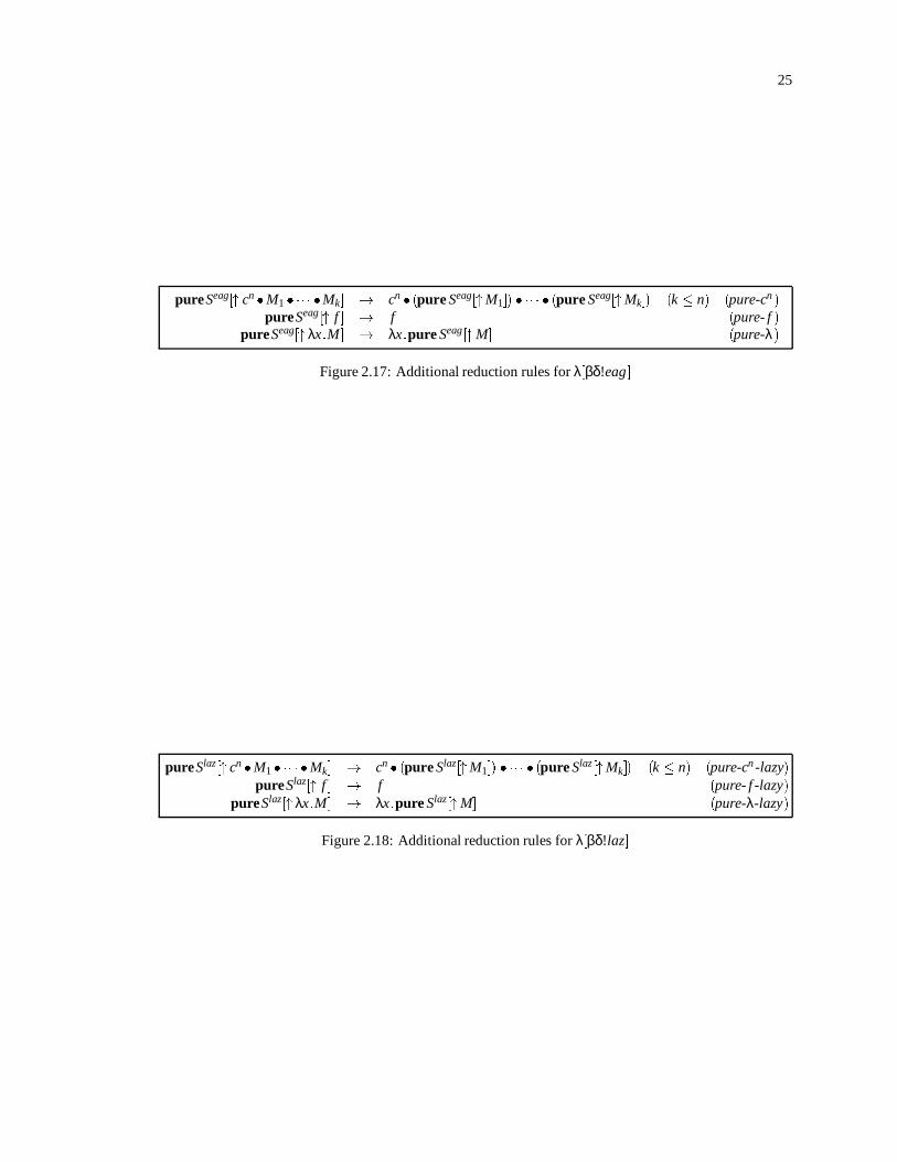
25

pureSeag[" cn M1 Mk] ! cn (pure Seag["M1]) (pure Seag["Mk]) (k n) (pure-cn )pureSeag[" f ] ! f (pure- f )

pureSeag[" λx:M] ! λx:pure Seag["M] (pure-λ)

Figure 2.17: Additional reduction rules for λ[βδ!eag]

pureSlaz[" cn M1 Mk] ! cn (pure Slaz["M1]) (pure Slaz["Mk]) (k n) (pure-cn -lazy)pureSlaz[" f ] ! f (pure- f -lazy)

pureSlaz[" λx:M] ! λx:pure Slaz["M] (pure-λ-lazy)

Figure 2.18: Additional reduction rules for λ[βδ!laz]

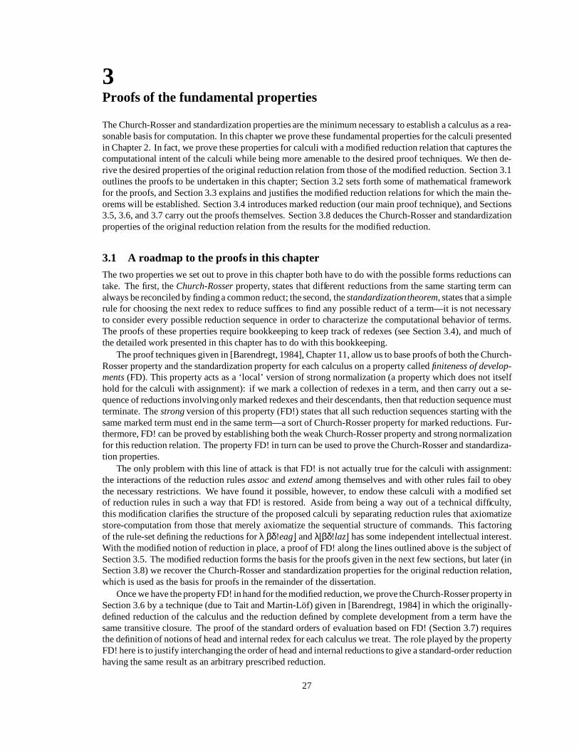
3Proofs of the fundamental properties

The Church-Rosser and standardization properties are the minimum necessary to establish a calculus as a rea-sonable basis for computation. In this chapter we prove these fundamental properties for the calculi presentedin Chapter 2. In fact, we prove these properties for calculi with a modified reduction relation that captures thecomputational intent of the calculi while being more amenable to the desired proof techniques. We then de-rive the desired properties of the original reduction relation from those of the modified reduction. Section 3.1outlines the proofs to be undertaken in this chapter; Section 3.2 sets forth some of mathematical frameworkfor the proofs, and Section 3.3 explains and justifies the modified reduction relations for which the main the-orems will be established. Section 3.4 introduces marked reduction (our main proof technique), and Sections3.5, 3.6, and 3.7 carry out the proofs themselves. Section 3.8 deduces the Church-Rosser and standardizationproperties of the original reduction relation from the results for the modified reduction.

3.1 A roadmap to the proofs in this chapterThe two properties we set out to prove in this chapter both have to do with the possible forms reductions cantake. The first, the Church-Rosser property, states that different reductions from the same starting term canalways be reconciled by finding a common reduct; the second, the standardizationtheorem, states that a simplerule for choosing the next redex to reduce suffices to find any possible reduct of a term—it is not necessaryto consider every possible reduction sequence in order to characterize the computational behavior of terms.The proofs of these properties require bookkeeping to keep track of redexes (see Section 3.4), and much ofthe detailed work presented in this chapter has to do with this bookkeeping.

The proof techniques given in [Barendregt, 1984], Chapter 11, allow us to base proofs of both the Church-Rosser property and the standardization property for each calculus on a property called finiteness of develop-ments (FD). This property acts as a ‘local’ version of strong normalization (a property which does not itselfhold for the calculi with assignment): if we mark a collection of redexes in a term, and then carry out a se-quence of reductions involvingonly marked redexes and their descendants, then that reduction sequence mustterminate. The strong version of this property (FD!) states that all such reduction sequences starting with thesame marked term must end in the same term—a sort of Church-Rosser property for marked reductions. Fur-thermore, FD! can be proved by establishing both the weak Church-Rosser property and strong normalizationfor this reduction relation. The property FD! in turn can be used to prove the Church-Rosser and standardiza-tion properties.

The only problem with this line of attack is that FD! is not actually true for the calculi with assignment:the interactions of the reduction rules assoc and extend among themselves and with other rules fail to obeythe necessary restrictions. We have found it possible, however, to endow these calculi with a modified setof reduction rules in such a way that FD! is restored. Aside from being a way out of a technical difficulty,this modification clarifies the structure of the proposed calculi by separating reduction rules that axiomatizestore-computation from those that merely axiomatize the sequential structure of commands. This factoringof the rule-set defining the reductions for λ[βδ!eag] and λ[βδ!laz] has some independent intellectual interest.With the modified notion of reduction in place, a proof of FD! along the lines outlined above is the subject ofSection 3.5. The modified reduction forms the basis for the proofs given in the next few sections, but later (inSection 3.8) we recover the Church-Rosser and standardization properties for the original reduction relation,which is used as the basis for proofs in the remainder of the dissertation.

Once we have the property FD! in hand for the modified reduction, we prove the Church-Rosser property inSection 3.6 by a technique (due to Tait and Martin-Lof) given in [Barendregt, 1984] in which the originally-defined reduction of the calculus and the reduction defined by complete development from a term have thesame transitive closure. The proof of the standard orders of evaluation based on FD! (Section 3.7) requiresthe definition of notions of head and internal redex for each calculus we treat. The role played by the propertyFD! here is to justify interchanging the order of head and internal reductions to give a standard-order reductionhaving the same result as an arbitrary prescribed reduction.

27

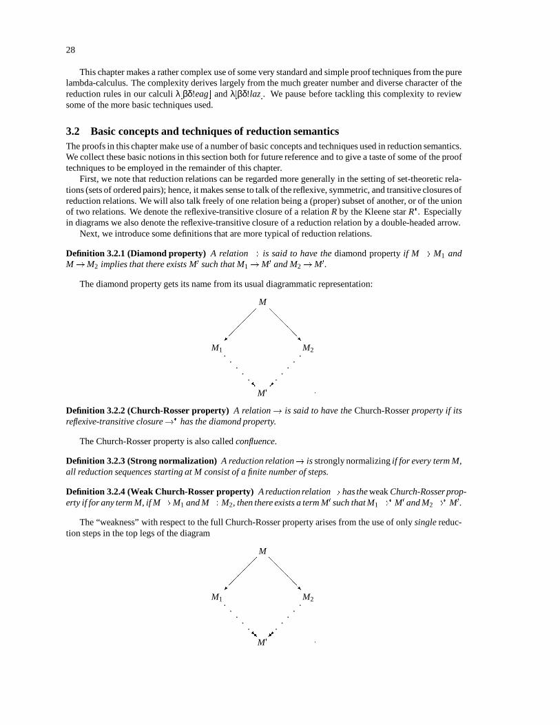
28

This chapter makes a rather complex use of some very standard and simple proof techniques from the purelambda-calculus. The complexity derives largely from the much greater number and diverse character of thereduction rules in our calculi λ[βδ!eag] and λ[βδ!laz]. We pause before tackling this complexity to reviewsome of the more basic techniques used.

3.2 Basic concepts and techniques of reduction semanticsThe proofs in this chapter make use of a number of basic concepts and techniques used in reduction semantics.We collect these basic notions in this section both for future reference and to give a taste of some of the prooftechniques to be employed in the remainder of this chapter.

First, we note that reduction relations can be regarded more generally in the setting of set-theoretic rela-tions (sets of ordered pairs); hence, it makes sense to talk of the reflexive, symmetric, and transitive closures ofreduction relations. We will also talk freely of one relation being a (proper) subset of another, or of the unionof two relations. We denote the reflexive-transitive closure of a relation R by the Kleene star R. Especiallyin diagrams we also denote the reflexive-transitive closure of a reduction relation by a double-headed arrow.

Next, we introduce some definitions that are more typical of reduction relations.

Definition 3.2.1 (Diamond property) A relation! is said to have the diamond property if M! M1 andM!M2 implies that there exists M0 such that M1!M0 and M2!M0.

The diamond property gets its name from its usual diagrammatic representation:

M

M1 M2

M0

@@@@R

..

..

..R

..

..

..

:

Definition 3.2.2 (Church-Rosser property) A relation! is said to have the Church-Rosser property if itsreflexive-transitive closure! has the diamond property.

The Church-Rosser property is also called confluence.

Definition 3.2.3 (Strong normalization) A reduction relation! is strongly normalizing if for every term M,all reduction sequences starting at M consist of a finite number of steps.

Definition 3.2.4 (Weak Church-Rosser property) A reduction relation! has the weak Church-Rosser prop-erty if for any term M, if M!M1 and M!M2, then there exists a term M0 such that M1!

M0 and M2! M0.

The “weakness” with respect to the full Church-Rosser property arises from the use of only single reduc-tion steps in the top legs of the diagram

M

M1 M2

M0

@@@@R

..

..

..RR

..

..

..

:

29

The weak Church-Rosser property is a convenient stepping-stone to proving the full Church-Rosser propertyfor some calculi because of the following standard result:

Proposition 3.2.5 (Newman) If a reduction relation! is both weakly Church-Rosser and strongly normal-izing, then it is Church-Rosser.

Proof: Standard: see [Barendregt, 1984], Proposition 3.1.25.

The proof of the weak Church-Rosser property for a calculus can usually be structured as two nested caseanalyses. First and outermost, we classify cases by the relative position of the two redexes—whether ∆1 and∆2 are identical, disjoint, or one is a subterm of the other. Second, we form a case for each pair of reductionrules by which ∆1 and ∆2 are redexes.

The standard argument for the outer case analysis is as follows:

Case (1) ∆1 and ∆2 are disjoint. In this case, each redex is trivially preserved when the other is reduced; re-ducing the preserved redex completes the diamond diagram.

Case (2) ∆1 and ∆2 are identical. In this case the diamond property can be satisfied by carrying out no reduc-tions on the lower legs of the diamond diagram.

Case (3) ∆1 contains ∆2 as a proper subterm. This case requires consideration of every pair of reduction rules,potentially yielding a number of subcases that is the square of the number of reduction rules. How-ever, we can usually avoid considering this many cases by using the notion of critical overlap orcritical pair from term-rewriting theory (see, for instance, [Klop, 1992]; the crucial lemma is from[Knuth and Bendix, 1970; Huet, 1980]). The necessary observation is that a redex contained insidea meta-variable of a reduction rule will just be carried along intact when rewriting according to therule. The intact redex is then still available for immediate reduction, so it is trivial to satisfy the dia-mond diagram. Only if the contained redex overlaps with the containing redex in a non-trivial way(by sharing some term-constructors) do we need to create a special case to establish that the reduc-tions by the redexes ∆1 and ∆2 can be reconciled. It should be noted both that a rule may have acritical overlap with itself and that two rules may have a critical overlap in more than one distinctway. One consequence of the definition of critical overlap is that rules which act on redexes definedin terms of disjoint sets of term-constructors cannot form critical pairs.

Some caution is required when applying critical-pair reasoning in the context of lambda-calculi. Inlambda-calculi, unlike in elementary term-rewriting systems, substitutable variables are part of theactual syntax of terms, not just meta-expressions for talking about terms. This means in particularthat it is no longer necessarily true that the term denoted by a meta-variable is carried along intact,because one or more of its free variables may be substituted via a β-reduction or similar rule. It isoften necessary to establish that relations are substitutive in order to use critical-pair reasoning whenthis occurs.

Case (4) ∆2 contains ∆1 as a proper subterm. This case can be argued by symmetry with Case 3 and so doesnot require separate consideration.

We close this section of basic techniques with a basic method for proving that a stepwise transformation ofterms must terminate in a finite number of steps. The technique is simply to define a function that maps termsto nonnegative integers in such a way that the allowed transformations always strictly decrease the value ofthe function. Such a process must bump into zero after a finite number of iterations.

3.3 Factoring the notion of reductionAmong the reduction rules defining the reduction relation! for λ[βδ!eag] and λ[βδ!laz], the rules assoc andextend are unusual in that they do not directly contribute to the semantic substance of the calculi. The rules β, δ,fuse, and assign-result directly model the intended notions of computation—substitution,primitive operations,and observation of assigned values, respectively. The rules bubble-assign and bubble-new assist the modeling

30

of assignment by the rule fuse. The rules assoc and extend, however, only rearrange the syntax of command-terms so that the other rules may apply. In fact, the way in which these rearrangements interact with eachother and with the other rules disrupts the effectiveness of the proof techniques to be used in Sections 3.4and 3.5; we will explain the problem when we come to introduce those techniques. Section 3.3.1 considersthe factoring-out of these rules as the basis for an equivalence relation on λ[βδ!eag]- and λ[βδ!laz]-terms; wethen turn our attention in Section 3.3.2 from the reduction relations formed by all the rules of the calculi toa modified relation that operates on the equivalence classes induced by assoc and extend. It should be notedthat this factoring of the notion of reduction is local to the present chapter, for we show in Section 3.8 that wecan recover the Church-Rosser and standardization properties for the original reduction relation from thosefor the factored notion.

3.3.1 The reduction relation!.

Certain crucial technical properties of the calculi introduced in Chapter 2 are more easily proved if we some-how take account of the fact that the rules assoc and extend act to reorder subterms of a command sequence butdon’t actually have any computational significance of their own. This subsection introduces the reduction re-lation!. (pronounced “association”) based on these rules alone and studies some of its important properties.The conversion relation based on this reduction relation identifies all command sequences having the samecommands in the same order, regardless of the way in which this sequence is built up from its subsequencesusing the operator .. For example, the terms (m1 .x2 m2).x3 (m3 .x4 m4) and m1 .x2 (m2 .x3 m3).x4 m4belong to the same equivalence class under this conversion relation. We will show, in fact, that the most eas-ily notated member of this equivalence class, m1 .x2 m2 .x3 m3 .x4 m4 , which is the!. -normal form of thetwo previously-mentioned terms, serves as a useful canonical representative of the entire equivalence class.

Note. For the remainder of this chapter, the unadorned reduction arrow!will refer to the original reductionrelations defined in Chapter 2 for the calculi λ[βδ!eag] and λ[βδ!laz].

Lemma 3.3.1 The reduction relation!. is weakly Church-Rosser.

Proof: It is sufficient to consider the cases in which the individual reduction rules assoc and extend have crit-ical overlaps with themselves or each other. The following is an list of such cases (determined by inspectionto be exhaustive), along with the diagrammatic evidence required for each case. There is a critical overlapbetween assoc and itself, and one between assoc and extend. There are no rewrite rules involving substitutionin the definition of!. , so critical-pair reasoning can be applied without modification.

Notation. The diagrams we use to convey this proof use a good deal of notation to keep track of redexes,an issue that will become more important in later proofs that use the same notation. In this notation, largehorizontal braces indicate the extent of the next redex to be reduced along some path in the diagram. A braceon top refers to the left-hand reduction path; one on the bottom, to the right-handpath. The redexes themselvesare marked by overliningor underlining the term-constructors that match the left-hand side of a reduction rule.The marks remain on the term-constructors until the corresponding rule is applied; the location of the bracesand of the lines are not intended to correspond. The arrow denoting the application of a rule that reduces amarked redex is marked the same way as the redex being reduced. Solid arrows denote reductions which aregiven in the hypotheses of a proposition; dotted arrows denote reductions which must be constructed to meeta proof obligation.

Case (1) ∆1: assoc; ∆2: assoc

31

The one possible overlap between the rule assoc and itself is the following:

z | ((N1 .x2 N2).x3 N3 )| z

.x4 N4

z | (N1 .x2 N2 ).x3 (N3 .x4 N4)

(N1 .x2 (N2 .x3 N3)).x4 N4| z

N1 .x2 ((N2 .x3 N3).x4 N4 )| z

N1 .x2 (N2 .x3 (N3 .x4 N4 ))

assoc

..............

assoc

@@@@@R

assoc

.

.

.

.

.

.?

assoc

..

..

..

..

assoc

:

Case (2) ∆1: assoc; ∆2: extend

Rule assoc overlaps rule extend as follows:

z | ((νv:N1 ).x2 N2| z

).x3 N3

z | (νv:N1).x2 (N2 .x3 N3)

(νv:(N1 .x2 N2 )).x3 N3| z

νv:((N1 .x2 N2 ).x3 N3)| z

νv:(N1 .x2 (N2 .x3 N3 ))

assoc

..............

extend

HHjextend

.

.

.

.

.

.?

extend

..

..

..

..

assoc

:

Since all critical overlaps between redexes can be reconciled, the weak Church-Rosser property follows bythe usual argument involving non-overlapping redexes given in Section 3.2.

Althoughwe must defer a complete discussion to Section 3.4, the diagrams used in the proof of Lemma 3.3.1contain the justification for the factoring of the reduction relation that we are now carrying out. The detail tonote is that the right-hand path in each diagram requires the reduction of a redex that was not present in theoriginal term in order to re-establish one of the original redexes.

Lemma 3.3.2 The reduction relation!. is strongly normalizing.

32

Proof: This is almost obvious, but we give a formal proof anyhow. We define a positive integral measureon terms that is strictly decreased by each assoc- or extend-reduction. This implies that every such reductionsequence must terminate.

We define the measure M [[ ]] via the equations

M [[x]] = 1M [[v]] = 1

M [[cn ]] = 1

M [[ f ]] = 1M [[M. x N]] = 2M [[M]]+M [[N]]

M [[νv:M]] = 1+M [[M]];

where it is understood that M [[ ]] is additive on all other compound terms. Note that M [[M]] is at least 1 forevery term M.

We now show that M [[ ]] decreases under!. ; that is, that if M!. N, then M [[M]] > M [[N]]. We have onecase to consider for each of the two reduction rules defining!. .

Case (1) assoc: (M1 .x2 M2).x3 M3 !. M1 .x2 M2 .x3 M3 .

In this case, we calculate

M [[(M1 .x2 M2).x3 M3 ]] = 2M [[M1 .x2 M2 ]]+M [[M3 ]]

= 2(2M [[M1 ]]+M [[M2 ]])+M [[M3 ]]

= 4M [[M1 ]]+2M [[M2 ]]+M [[M3 ]]

> 2M [[M1 ]]+2M [[M2 ]]+M [[M3 ]]

= M [[M1 .x2 M2 .x3 M3 ]]:

Case (2) extend: (νv:M1).x2 M2 !. νv:M1 .x2 M2 .

In this case, we calculate

M [[(νv:M1).x2 M2 ]] = 2M [[νv:M1 ]]+M [[M2 ]]

= 2M [[M1 ]]+M [[M2 ]]+2

> 2M [[M1 ]]+M [[M2 ]]+1

= M [[νv:M1 .x2 M2 ]]:

In the first case, the inequality depends on knowing that M [[M]] is always greater than zero. The decreasein M [[M]], which we have demonstrated for redexes only, extends to entire terms by noting that the measureof subterms always contributes positively to the measure of a superterm. Since M [[ ]] decreases at every stepyet remains bounded below by 0, the number of steps must be finite.

Theorem 3.3.3 The reduction relation!. is Church-Rosser.

Proof: This follows by Newman’s Lemma (Proposition 3.2.5) from Lemmas 3.3.1 and 3.3.2.

Notation 3.3.4 We will denote the!. -normal form of a term M by #. [M].

Definition 3.3.5 The equivalence relation.=, association equivalence, is the equivalence closure of!. .

Proposition 3.3.6 The relation.= is decidable.

Proof: The confluence of!. implies that terms related by.= share a common, unique!. -normal form. Since

all!. -reduction sequences terminate, it is sufficient to reduce two candidate terms to!. -normal form andcheck for syntactic equivalence.

The next proposition establishes that the reduction relation!. possesses a standard reduction order forreduction to normal form.

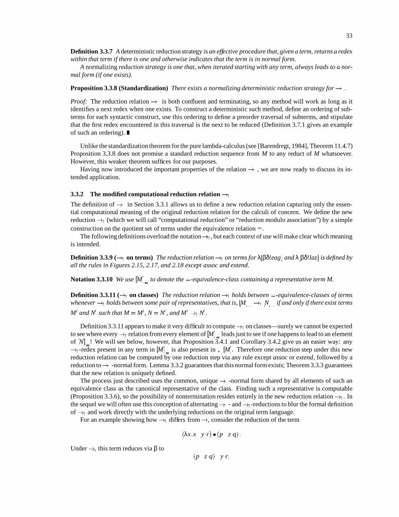
33

Definition 3.3.7 A deterministic reduction strategy is an effective procedure that, given a term, returns a redexwithin that term if there is one and otherwise indicates that the term is in normal form.

A normalizing reduction strategy is one that, when iterated starting with any term, always leads to a nor-mal form (if one exists).

Proposition 3.3.8 (Standardization) There exists a normalizing deterministic reduction strategy for!. .

Proof: The reduction relation!. is both confluent and terminating, so any method will work as long as itidentifies a next redex when one exists. To construct a deterministic such method, define an ordering of sub-terms for each syntactic construct, use this ordering to define a preorder traversal of subterms, and stipulatethat the first redex encountered in this traversal is the next to be reduced (Definition 3.7.1 gives an exampleof such an ordering).

Unlike the standardization theorem for the pure lambda-calculus (see [Barendregt, 1984], Theorem 11.4.7)Proposition 3.3.8 does not promise a standard reduction sequence from M to any reduct of M whatsoever.However, this weaker theorem suffices for our purposes.

Having now introduced the important properties of the relation!. , we are now ready to discuss its in-tended application.

3.3.2 The modified computational reduction relation!!

The definition of!. in Section 3.3.1 allows us to define a new reduction relation capturing only the essen-tial computational meaning of the original reduction relation for the calculi of concern. We define the newreduction!! (which we will call “computational reduction” or “reduction modulo association”) by a simpleconstruction on the quotient set of terms under the equivalence relation .

=.The followingdefinitions overload the notation!! , but each context of use will make clear which meaning

is intended.

Definition 3.3.9 (!! on terms) The reduction relation!! on terms for λ[βδ!eag] and λ[βδ!laz] is defined byall the rules in Figures 2.15, 2.17, and 2.18 except assoc and extend.

Notation 3.3.10 We use [M] .

=to denote the

.=-equivalence-class containing a representative term M.

Definition 3.3.11 (!! on classes) The reduction relation!! holds between.=-equivalence-classes of terms

whenever!! holds between some pair of representatives, that is, [M] .

=!! [N] .

=if and only if there exist terms

M0 and N0 such that M.= M0, N

.= N0 , and M0!! N0 .

Definition 3.3.11 appears to make it very difficult to compute!! on classes—surely we cannot be expectedto see where every!! relation from every element of [M] .

=leads just to see if one happens to lead to an element

of [N] .

=! We will see below, however, that Proposition 3.4.1 and Corollary 3.4.2 give us an easier way: any

!! -redex present in any term in [M] .

=is also present in #. [M]. Therefore one reduction step under this new

reduction relation can be computed by one reduction step via any rule except assoc or extend, followed by areduction to!. -normal form. Lemma 3.3.2 guarantees that this normal form exists; Theorem 3.3.3 guaranteesthat the new relation is uniquely defined.

The process just described uses the common, unique!. -normal form shared by all elements of such anequivalence class as the canonical representative of the class. Finding such a representative is computable(Proposition 3.3.6), so the possibility of nontermination resides entirely in the new reduction relation!! . Inthe sequel we will often use this conception of alternating!. - and!! -reductions to blur the formal definitionof!! and work directly with the underlying reductions on the original term language.

For an example showing how!! differs from!, consider the reduction of the term

(λx:x. y r) (p. z q):

Under!, this term reduces via β to(p. z q) .y r;

34

which is itself an assoc-redex; reducing this redex is counted as a second reduction to the final result

p. z q. y r:

In contrast, under!! we are working with.=-equivalence classes of terms. The intial term is in

.=-normal

form; its reduct, however, contains the!. -redex just pointed out. The!-reductions induce the one-step!! -reduction

[(λx:x. y r) (p. z q)] .=!! [p. z q. y r ] .

=:

Some precedents. The singling out of!. as a non-computational subset of the overall reduction relation issomewhat reminiscent of the “structural congruences” employed in the exposition of the polyadic π-calculusin [Milner, 1991]. There (as here) the axioms in question are essential for definining computations, but do notthemselves model the progress of a computation.

There is also an analogy between the definition of!! and the α-renaming convention adopted in [Baren-dregt, 1984]. Under the α-renaming convention we agree to give all bound and free variables different namesbefore each reduction step. This convention sweeps the complex process of renaming variables under the rug,but allows us to avoid painfully endless invocations of the phrase “up to α-equivalence” as well as numerousside-conditions to the effect that a particular variable does not occur free in a certain subterm. Terms are thusregarded as representatives of their α-equivalence class, the classes being the true computational objects.

Like the α-renaming convention, the definition of!! requires us to think in terms of equivalence classesof terms. This definition folds this (slight) complexity into the basic notion of reduction, but allows us toavoid complexity elsewhere. When using!! , we consider terms as representatives of their!. -equivalenceclasses, the classes being the true computational objects. Corollary 3.4.2 provides the foundation for this viewof!! -reduction.

3.4 Keeping track of redexesThe proofs of the Church-Rosser and standardization properties depend ultimately on the details of the waysin which different choices of reductions can be reconciled. Proving the Church-Rosser property requires thatsuch reconciliations always exist; proving standardization requires that interchanging the order of reductionsso as to fit the definition of standard order is always possible. In this section we present the basic definitionsfor keeping track of reductions in support of these proofs. In Section 3.5 we apply these techniques to gatherinformation about the reduction relations in λ[βδ!eag] and λ[βδ!laz].

3.4.1 Marked reductions

The basic tool for keeping track of redexes, already introduced in the diagrams for the proof of Lemma 3.3.1,is to label the term-constructors of redexes with distinctivemarks.1 The marks for a particular redex are erasedwhen that particular redex is reduced but not when other redexes are reduced. For example, the following termhas two β-redexes, marked with overlines and underlines respectively:

(λx:(λy:y) x) z:

A β-redex is specified in terms of two syntactic term constructors: one for the application term-constructor,one for the λ-abstraction term-constructor. Both are marked, and both disappear when the redex is reduced.When the underlined redex above is reduced, the resulting marked term is

(λy:y) z:

The formal specification of the concept of marked redexes and marked reductions is best left as a sketch—a full development yields no great advantage in precision. The addition of marks creates a new language of

1The marking technique presented here is adapted from [Barendregt, 1984], Chapter 11.

35

terms, with a lifting function that embeds terms from the original language into the marked language as un-marked terms, and an erasing function that provides a mapping in the reverse direction by forgetting the marks.Reduction rules from the unmarked language are lifted to the marked language as already discussed; the addi-tion of these rules turns the marked language into a calculus. Every reduction sequence in the marked calculusis reflected in the unmarked calculus by erasing the marks.

The converse, that all unmarked reduction sequences can be lifted into the marked calculus, is not true;this fact underlies the technical usefulness of the marking technique. Of course, it takes a theorem to show thatthis converse does not hold, but the basic idea is easy: reductions destroy marks but cannot create them, sosequences consisting only of marked reductions are finite. On the other hand, untyped lambda-calculi admitinfinite reduction sequences.

The syntactic form of our store-computation redexes introduces a complication not present in the basiclambda-calculus λ[βδ]. In λ[βδ], β- and δ-redexes cannot overlap in the sense of sharing a syntactic term-constructor. For example, any β- or δ-redex in the term (λx:M) N over and above the redex that is the rootof the term must lie entirely within one of the subterms denoted by the metavariables M and N. It is not soin either of our lambda-calculi with assignment. An example is the term ("N1 .x2 N2) .x3 N3 , in which wehave marked with an underline the constructors of terms defining an assoc-redex and have marked with a lineabove the constructors of terms defining a unit-redex. We have given the term constructor .x2 both marks. Toaccommodate overlapping redexes, we must formally require that our terms be marked with sets of marks, andthat the mark for a particular redex appear in the mark-set for all and only those subterms which characterizethe redex. We call terms marked with the empty set unmarked even when they are considered as elements ofa marked calculus. The uses of the marking apparatus that actually appear in the ensuing proofs actually useno more than two marks.

The marking technique as presented so far is only applicable to a calculus defined directly in terms ofreduction rules. In order to use marked terms in the proofs we actually want to carry out, we need to showhow marked reductions interact with the definition of!! in terms of .

=-equivalence classes. This adaptationis the topic of the next subsection.

3.4.2 Interaction of!. with marked computational reduction

We now state and prove a result that lets us reason with the computational reduction!! in a fairly simple man-ner. Although the method of defining!! by carrying out a!. -normalization after every!! -step is concep-tually simple, it can lead to complicated proofs. The following result gives us some leeway in the placementof!. -steps with respect to!! -steps when constructing proofs: it shows that we can always choose to per-form some of the!. -reductions before a!! -reduction without changing the interpretation of the reductionsequence in terms of .

=-equivalence classes.

Proposition 3.4.1 (Commutation of association) Suppose we have M!! N via reduction of a marked redex∆, and suppose also that M!. M0: Then there exist terms M00 and N0 such that M0!.

M00, N!.N0 , and

M00!! N0 by reducing ∆00 , where ∆00 is the residual of ∆ in M00.

36

M

N M0

M00

N0

!!

∆

..

..

..

..

..

..

..

..

..

.R

!.

R

@@@@@R

!.

..

..

..

..R

!.

R.

..

..

..

.

!!

..

..

..

..

∆00

:

Proof: The existence of ∆00 is part of what we have to prove. It is possible that a residual of ∆ might not bea redex, but the proof will show that it will always be possible to re-establish redexhood via a further!. -reduction. This fact is what makes Proposition 3.4.1 useful.

Following the general pattern of argument given in Section 3.2, we argue by a case analysis on the relativepositions of the!. - and!! -redexes, and also consider the particular rules defining the redexes.

The arguments reducing the case analysis to cases of critical overlap are valid in this case because thereduction rules defining !. are obviously substitutive. We now proceed to examine the critical overlapsbetween !. -rules and !! -rules. We prove each case by means of a diagram in which we mark the term-constructors of the redex ∆. The diagrams themselves correspond to the diagram that states the theorem.

Case (1)

z | ("M1 .x2 M2| z

).x3 M3

z | "M1 .x2 (M2 .x3 M3)

[M1=x2 ](M2 .x3 M3) ([M1=x2 ]M2).x3 M3

?

unit

@@@@R

assoc

..

..

..

..

unit

The syntactic identity ([M1=x2 ]M2).x3 M3 [M1=x2 ](M2 .x3 M3) holds because there can be nooccurrences of x2 in M3, which was outside the scope of x2 in the original term M. The α-renamingconvention (Section 2.1) assures that no free occurrences of x2 have been introduced.

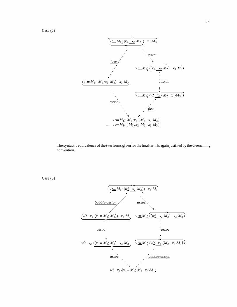
37

Case (2)

z | (v := M1; (v? .x2 M2)| z

).x3 M3

v :=M1; (z | (v? .x2 M2).x3 M3)

z | v :=M1; (v? .x2 (M2 .x3 M3 ))

(v := M1; [M1=x2 ]M2).x3 M3| z

v :=M1; [M1=x2 ](M2 .x3 M3) v :=M1; ([M1=x2 ]M2 .x3 M3)

fuse

......

.....

assoc

@@@@R

assoc

.

.

.

.

.

.?

assoc

..

..

..

..

fuse

The syntactic equivalence of the two forms given for the final term is again justified by the α-renamingconvention.

Case (3)

z | (v := M1; (w? .x2 M2)| z

).x3 M3

v :=M1;z | ((w? .x2 M2).x3 M3 )

z | v :=M1; (w? .x2 (M2 .x3 M3))

(w? .x2 (v := M1; M2)).x3 M3| z

w?.x2 ((v := M1; M2).x3 M3)| z

w?.x2 (v := M1; M2 .x3 M3)

@@@@R

assoc

.

.

.

.

.

.?

assoc

..

..

..

..

.

bubble-assign

bubble-assign

.

.

.

.

.

.?

assoc

..

..

..

..R

assoc

38

Case (4)

z | (v := M1 .x2 M2| z

).x3 M3 ; (x2 2 fv M2)

z | v :=M1 .x2 (M2 .x3 M3);(x2 2 fv M2)

(v := M1; [( )=x2 ]M2).x3 M3 v :=M1; [( )=x2 ](M2 .x3 M3)

@@@@Rassoc

..

..

..

.

assign-result

?

assign-result

The last reduction again depends on the fact that there can be no occurrences of x2 in M3.

Case (5)

z | (νv:(w? .x1 M1)| z

).x2 M2

νv:(z | (w? .x1 M1).x2 M2)

z | νv:(w? .x1 (M1 .x2 M2))

(w? .x1 νv:M1).x2 M2| z

w?.x1 (νv:M1).x2 M2| z

w?.x1 (νv:(M1 .x2 M2))

@@@@R

extend

.

.

.

.

.

.?

assoc

..

..

..

..

.

bubble-new

bubble-new

.

.

.

.

.

.?

assoc

..

..

..

..R

extend

Case (6) We now consider the purification rules. For λ[βδ!eag], the form of the prefixes Seag[] precludes anyoverlaps between pure-eager-redexes and!. -redexes—the store-prefixes allowed in pure-eager-redexes are in!. -normal form. We thus have only to consider pure-lazy-redexes. We first consider

39

the interaction of pure-lazy with extend.

z |

pureSlaz1 [(νv:M) .x Slaz

2 [" (λy:N)]| z

]

λy:pure Slaz1 [(νv:M) .x Slaz

2 ["N]| z

]z |

pureSlaz1 [νv:M. x Slaz

2 [" (λy:N)]]

λy:pure Slaz1 [νv:M. x Slaz

2 ["N]]

pure-lazy

..

..

..

..R

extend

@@@@Rextend

..

..

..

..

.

pure-lazy

The cases involving the rules for purifying constructed values and primitives, as well as the corre-sponding cases involving assoc, behave analogously.

The completion of this case analysis concludes the proof of Proposition 3.4.1.

As a corollary to Proposition 3.4.1, we can show that a!. -normal form contains every!! -redex presentin any member of its .

=-equivalence class. Hence these normal forms make a handy canonical representativeof the class when one is needed.

Corollary 3.4.2 (Completeness of!. -normal form) If ∆ is a!! -redex within any term in a.=-equivalence

class [M] .

=, then there exists a residual ∆0 of ∆ within the normal form #. [M], and ∆0 is a redex. Moreover, if

M!! M0 by reducing ∆ and #. [M]!! M00 by reducing ∆0, then M0!.M00.

Proof: In diagram form, the corollary states

M 2 [M] .=

M0 2 [M0 ] .=

#. [M]

M00 2 [M00 ] .=

∆@@@@@@RR

..

..

..

..

.RR

..

...

...

..

∆0

:

We need only stitch together, from upper left to lower right, occurrences of the diagram given in the state-ment of Proposition 3.4.1. At each step, we re-establish a residual of ∆ as a redex using!. -reductions only,hence we stay within the equivalence class. Since!. is strongly normalizing and Church-Rosser, the pro-cess terminates at #. [M]. Starting this process at every element of [M] .

=shows that every marked!! -redex

of every term in the equivalence class is represented by a residual redex in the normal form that characterizesthe class.

It should be noted that Corollary 3.4.2 does not state that M00 #. [M0 ]: this isn’t true. For an example,consider the term

(λy:y. x2 z2) z1 .x3 z3 :

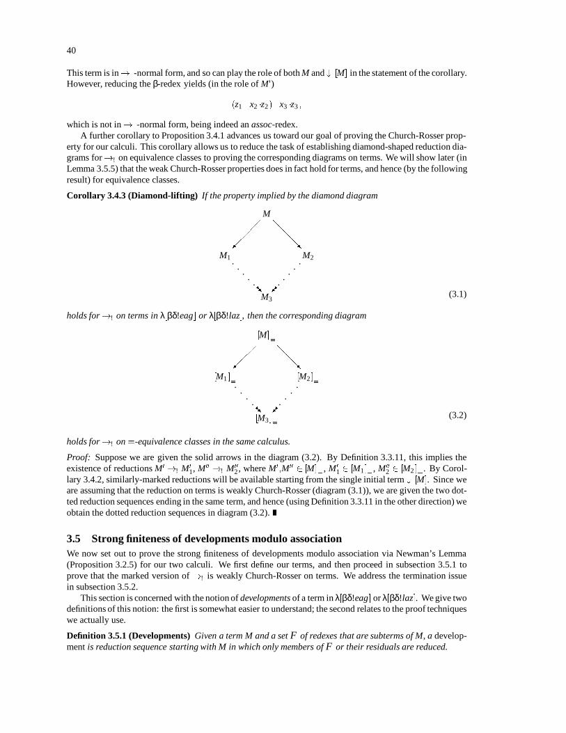
40

This term is in!. -normal form, and so can play the role of both M and #. [M] in the statement of the corollary.However, reducing the β-redex yields (in the role of M0)

(z1 .x2 z2).x3 z3 ;

which is not in!. -normal form, being indeed an assoc-redex.A further corollary to Proposition 3.4.1 advances us toward our goal of proving the Church-Rosser prop-

erty for our calculi. This corollary allows us to reduce the task of establishing diamond-shaped reduction dia-grams for!! on equivalence classes to proving the corresponding diagrams on terms. We will show later (inLemma 3.5.5) that the weak Church-Rosser properties does in fact hold for terms, and hence (by the followingresult) for equivalence classes.

Corollary 3.4.3 (Diamond-lifting) If the property implied by the diamond diagram

M

M1 M2

M3

..

..

..RR

@@@@R

..

..

.. (3.1)

holds for!! on terms in λ[βδ!eag] or λ[βδ!laz], then the corresponding diagram

[M] .

=

[M1 ] .= [M2 ] .=

[M3 ] .=

..

..

.RR

@@@R

..

..

.(3.2)

holds for!! on.=-equivalence classes in the same calculus.

Proof: Suppose we are given the solid arrows in the diagram (3.2). By Definition 3.3.11, this implies theexistence of reductions M0!! M0

1, M00 !! M00

2, where M0;M00 2 [M] .

=, M0

1 2 [M1 ] .=, M00

2 2 [M2 ] .=. By Corol-lary 3.4.2, similarly-marked reductions will be available starting from the single initial term #. [M]. Since weare assuming that the reduction on terms is weakly Church-Rosser (diagram (3.1)), we are given the two dot-ted reduction sequences ending in the same term, and hence (using Definition 3.3.11 in the other direction) weobtain the dotted reduction sequences in diagram (3.2).

3.5 Strong finiteness of developments modulo associationWe now set out to prove the strong finiteness of developments modulo association via Newman’s Lemma(Proposition 3.2.5) for our two calculi. We first define our terms, and then proceed in subsection 3.5.1 toprove that the marked version of!! is weakly Church-Rosser on terms. We address the termination issuein subsection 3.5.2.

This section is concerned with the notion of developments of a term in λ[βδ!eag] or λ[βδ!laz]. We give twodefinitions of this notion: the first is somewhat easier to understand; the second relates to the proof techniqueswe actually use.

Definition 3.5.1 (Developments) Given a term M and a set F of redexes that are subterms of M, a develop-ment is reduction sequence starting with M in which only members of F or their residuals are reduced.

41

Definition 3.5.2 (Developments) Given a term M in the marked calculus, a development is a sequence ofmarked reductions starting with M.

In both cases, we sometimes use the term “development” informally to refer to the final term in the reduc-tion sequence that forms a development.

Corresponding to the two definitions of developments, we give two definitions of the important notion ofcomplete development.

Definition 3.5.3 (Complete developments) A complete development of a term M relative to a set of redexesF is one in which all the members of F are reduced.

Definition 3.5.4 (Complete developments) A complete development of a term M is one in which all marksare erased.

The weak finite-developments property can perhaps best be thought of in terms of its contrapositive state-ment: any infinite reduction sequence must create new redexes.

3.5.1 The weak Church-Rosser property

In this subsection we establish that marked !! -reductions for λ[βδ!eag] and λ[βδ!laz] are weakly Church-Rosser on terms; Corollary3.4.3 will then establish the weak Church-Rosser property for marked!! on equiv-alence classes.

Lemma 3.5.5 The weak Church-Rosser property holds for the calculi λ[βδ!eag] and λ[βδ!laz] under marked!! -reduction on

.=-equivalence classes.

Proof: We consider all the critical overlaps between all the!! -rules in both our calculi; we show that in everycase the diamond can be completed. In contrast with the proof of Lemma 3.3.1, we are now dealing with rulesinvolvingsubstitutionso we cannot rely completely on critical-pair reasoning. Instead, we will have to accountcarefully for the interaction of substitutions arising from β-, unit-, fuse-, and assign-result-redexes.

Case (1): ∆1: β; ∆2: βThere are two ways a β-redex can be embedded within another: in the function subterm or in theargument subterm of the redex’s application. We consider the two cases separately.

(i) The first way in which two β-redexes can interact has the inner redex within the function-subterm of the outer redex.

z |

(λx1 :C[(λx2 :P2)Q2| z

])Q1

[Q1=x1 ]C[z |

(λx2 :P2)Q2]

([Q1=x1 ]C)[z |

(λx2 :[Q1=x1 ]P2) [Q1=x1 ]Q2]

(λx1 :C[[Q2=x2 ]P2 ])Q1| z

([Q1=x1 ]C)[[[Q1=x1 ]Q2=x2 ]([Q1=x1 ]P2 )] ([Q1=x1 ]C)[[Q1=x1 ] [Q2=x2 ]P2 ] [Q1=x1 ]C[[Q2=x2 ]P2 ]

β

..

..

.Rβ

@@@@@R

β

..

..

..

β

This diagram is rendered nonobvious by the fact that substitution is not a term-constructorbut rather a meta-level operator that denotes the term that is the result of the substitution. The

42

second form of the intermediate term on the left-hand leg of the diamond diagram above em-phasises this fact, and the equivalence in the final term in the diagram is a consequence of theSubstitution Lemma (Lemma 2.1.2). We use the notation ([M=x]C)[ ] to stand for the contextthat is derived from the context C[ ] by substituting as indicated.

(ii) The second way in which two β-redexes may interact has the inner redex in the argument termof the outer redex. The following diagram shows how the requirements of the weak Church-Rosser property are established in this case:

z |

(λx1 :P1)C[(λx2 :P2)Q2| z

]

[C[z |

(λx2 :P2 )Q2]=x1 ]P1 (λx1 :P1)C[[Q2=x2 ]P2 ]| z

[C[[Q2=x2 ]P2 ]=x1 ]P1

β

..

..

..

..

..R

β

R

@@@@@R

β

..

..

..

..

β

:

Here the lower-left arrow in the diamond has a double head because there may be multipleoccurrences of x1 in P1 , leading to multiple occurrences of the second β-redex to reduce.

All the other interactions of rule β with other reduction rules follow one or the other of these pro-totypes, so we do not work out all the diagrams for those cases explicitly.

Case (2): ∆1: β; ∆2: δ We give only the case in which the β-redex encloses the δ-redex. The case in which theenclosure relationship is reversed presents no difficulties due to substitution. We also give only theform of δ-rule dealing with an abstraction as an argument, since the rules for constructed argumentshave the same form.

z | (λx1 :C[ f (λy:M)

| z ])Q

[Q=x1 ]C[z | f (λy:M)]

([Q=x1 ]C)[z | f (λy:[Q=x1 ]M)]

(λx1 :C[Nf (λy:M)])Q| z

[Q=x1 ]C[Nf (λy:M)] ([Q=x1 ]C)[Nf (λy:[Q=x1 ]M)]

β

@@@@@R

δ

..

..

..R

δ

..

..

..

.β

Case (3): ∆1: unit; ∆2: any

The rule unit behaves just like β, so this case is proved in the same manner as Case 1.

Case (4): ∆1: fuse; ∆2: any

Case (5): ∆1: bubble-assign; ∆2: any

43

Case (6): ∆1: assign-result; ∆2: any

Case (7): ∆1: bubble-new; ∆2: any

There are no critical overlaps when any of the just-mentioned rules define the outer redex, so com-pleting the diamond to show the weak Church-Rosser property is trivial in all these cases.

Case (8): ∆1: pure-eager or pure-lazy; ∆2: any

The purification rules clearly have no overlaps with the rules β or δ, since the left-hand-sides arebased on different syntactic constructors. Also, since the purification rules contain no nested in-stance of pure, there is no overlap between purification rules and themselves. We are thus reducedto considering interactions between command-related rules on the one hand and purification ruleson the other.

In order to do this, we must consider the particular form of the store-contexts S[] for each calculus.For the eager calculus, we have

Seag[] ::= []j νv:Seag []j v :=M; Seag[];

It is clear from this definition that eager store-contexts do not overlap with rule unit, since thesecontexts can only have assignments to the left of a . operator. Nor can eager store-contexts overlapwith the left-hand-sides of the rules fuse, bubble-assign, identical, or not identical—by design, allthe reduction potential of an eager store-context has been exhausted. Since there are no overlapsinvolving pure-eager, there is no need to consider this rule in detail to establish the weak Church-Rosser property.

For λ[βδ!laz] with its purification rules pure-lazy, the situation is different. Equally by design, thelazy store-contexts Slaz[] can contain redexes that overlap with the context’s command sequence.We now consider each such possible overlap.

We simplify our consideration of these cases in two ways. First, we write these cases with only theminimal amount of store-context necessary to show the overlap; it is not hard to see that the con-structions hold when the overlaps occur in the midst of longer store-contexts. Second, we consideronly the purification rule applying to abstractions: this saves us the slight complication arising fromthe duplication of the pure-context that is prescribed by the rule pure-lazy when the result value is anapplication of a constructor of more than one argument. This duplication requires that the lower-leftleg of the corresponding diamond be a multistep reduction consisting of one independent applica-tion of the non-pure rule for each occurrence of the pure-context. The essential reasoning, however,is conveyed by the following simple cases.

(i) ∆1: pure-lazy; ∆2: unit

purez |

("M1).x " (λy:M2)| z

λy:pure ("M1).x "M2| z

z | pure[M1=x] " (λy:M2)

z | pure" (λy:[M1=x]M2)

λy:pure " [M1=x]M2

pure-lazy@@@Runit

..

..

..

..R

unit

..

..

..

.

pure-lazy

44

(ii) ∆1: pure-lazy; ∆2: fuse

purez |

v :=N; v? .x " (λy:M)| z

λy:purez |

v :=N; v? .x "M

z | purev :=N; [N=x] (" (λy:M))

z | purev :=N; "(λy:[N=x]M)

λy:pure v :=N; "([N=x]M)

pure-lazy@@@Rfuse

..

..

..

..

..R

fuse

..

..

..

.

pure-lazy

(iii) ∆1: pure-lazy; ∆2: bubble-assign

purez |

v :=N; w?.x " (λy:M)| z

λy:pure v :=N; w?.x "M| z

z | purew?.x v := N; " (λy:M)

λy:pure w?.x v := N; "M

pure-lazy@@@@R

bubble-assign

..

..

..

..R

bubble-assign

..

..

..

..

.

pure-lazy

(iv) ∆1: pure-lazy; ∆2: assign-result

purez | v :=N .x " (λy:M)

| z

λy:pure v :=N .x "M| z

z | purev :=N; [( )=x] (" (λy:M))

z | purev :=N; "(λy:[( )=x]M)

λy:pure v :=N; " [( )=x]M

pure-lazy@@@Rassign-result

..

..

..

..R

assign-result

..

..

..

.

pure-lazy

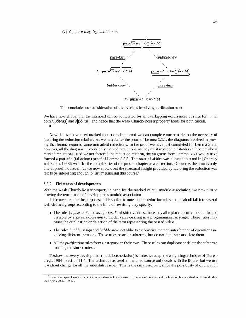
45

(v) ∆1: pure-lazy; ∆2: bubble-new

purez |

νv:w? .x " (λy:M)| z

λy:purez |

νv:w? .x "M purew?.x νv:" (λy:M)| z

λy:pure w?.x νv:"M

pure-lazy@@@@@R

bubble-new

..

..

..

..

..R

bubble-new

..

..

..

..

pure-lazy

This concludes our consideration of the overlaps involving purification rules.

We have now shown that the diamond can be completed for all overlapping occurrences of rules for!! inboth λ[βδ!eag] and λ[βδ!laz], and hence that the weak Church-Rosser property holds for both calculi.

Now that we have used marked reductions in a proof we can complete our remarks on the necessity offactoring the reduction relation. As we noted after the proof of Lemma 3.3.1, the diagrams involved in prov-ing that lemma required some unmarked reductions. In the proof we have just completed for Lemma 3.5.5,however, all the diagrams involve only marked reductions, as they must in order to establish a theorem aboutmarked reductions. Had we not factored the reduction relation, the diagrams from Lemma 3.3.1 would haveformed a part of a (fallacious) proof of Lemma 3.5.5. This state of affairs was allowed to stand in [Oderskyand Rabin, 1993]; we offer the complexities of the present chapter as a correction. Of course, the error is onlyone of proof, not result (as we now show), but the structural insight provided by factoring the reduction wasfelt to be interesting enough to justify pursuing this course.2

3.5.2 Finiteness of developments

With the weak Church-Rosser property in hand for the marked calculi modulo association, we now turn toproving the termination of developments modulo association.

It is convenient for the purposes of this section to note that the reduction rules of our calculi fall into severalwell-defined groups according to the kind of rewriting they specify:

The rules β, fuse, unit, and assign-result substitutive rules, since they all replace occurrences of a boundvariable by a given expression to model value-passing in a programming language. These rules maycause the duplication or delection of the term representing the passed value.

The rules bubble-assign and bubble-new, act alike to axiomatize the non-interference of operations in-volving different locations. These rules re-order subterms, but do not duplicate or delete them.

All the purification rules form a category on their own. These rules can duplicate or delete the subtermsforming the store context.

To show that every development (moduloassociation) is finite, we adapt the weighting technique of [Baren-dregt, 1984], Section 11.4. The technique as used in the cited source only deals with the β-rule, but we useit without change for all the substitutive rules. This is the only hard part, since the possibility of duplication

2For an example of work in which an alternative tack was chosen in the face of the identical problem with a modified lambda-calculus,see [Ariola et al., 1995].

46

W [[xn ]] = nW [[cn ]] = 1W [[ f n ]] = n

W [[λx:M]] = W [[M]]

W [[M1 M2]] = W [[M1 ]]+W [[M2 ]]

W [[νv:w? .x M]] = 1+W [[w? .x νv:M]]W [[v== w]] = 1+W [[λx:λy:y]]W [[v== v]] = 1+W [[λx:λy:x]]

W [[v := M1; w?.x2 M2 ]] = 1+W [[w? .x2 v := M1; M2]]

W [[pure Seag[" (cn M1 Mk)]]] = 1+W [[cn (pure Seag["M1]) (pure Seag["Mn]) ]]

W [[pure Slaz[" (cn M1 Mk)]]] = 1+W [[cn (pure Slaz["M1]) (pure Slaz["Mn]) ]](and so forth for the other pure rules)

W [[ ]] is additive on the subterms of all other terms.

Figure 3.1: Definition of the weight function.

of subterms in these reductions leads to some concern that the duplication of marked redex subterms mightoutrun their elimination through marked reductions. That this cannot actually happen is not obvious and is thepoint of the present proof.

For all the other rules, we merely count the number of marked redexes in the start term of the developmentin the weight of a term.

The weight function W [[]] on marked terms is defined in Figure 3.1. The function W [[]] is actually definedon a slightly modified calculus in which variables and primitive function names bear weights: the notion oferasing weights to recover the original calculus is straightforward from an informal description. Note thatW [[M]] is always at least 1. The definition of W [[]] is designed to decrease on each reduction of a marked redex.For substitutive redexes, this means that it should be possible to arrange to have the weighted occurrence ofthe substitution variable have a greater weight than the substituted expression; this is the reason for havingweighted variables. For δ-redexes, we want to be able to weight the primitive function name more heavilythan anything that might replace it. For the remaining kinds of redex, we just define the weight to be 1 greaterthan the reduced form.3

We will be concerned only with terms whose weightings have a special property contrived to make reduc-tions involving substitution and primitive function definitions decrease the weight of a term. The followingdefinition requires that substitution reductions must reduce the weight of a term. There are five cases becausethe calculi λ[βδ!eag] and λ[βδ!laz] have five kinds of substitutive redex.

Definition 3.5.6 A term M has a decreasing weighting if the following conditions on marked-redex subtermsall hold:

1. for all marked β-redex subterms (λx:M1)M2, for all xn in M1, we have n > W [[M2 ]],

2. for all marked δ-redex subterms fn V for which δ( f ;V) is defined, we have n+W [[V]] > W [[δ( f ;V)]],

3. for all marked unit-redex subterms "M1 .x2 M2 , we have, for all x2n in M2, n > W [[M1 ]],

4. for all marked fuse-redex subterms v :=M1; v? .x2 M2 , for every free occurrence of x2n in M2, we have

n > W [[M1 ]]

3In [Odersky and Rabin, 1993] the authors expend a great deal of effort in designing a weight function that decreases under evenstatically unknownpure-eager-reductions. This is unnecessary—all the relevant redexesmust be known in advance in order to be marked.

47

5. for all marked assign-result-redex subterms (v := M1 .x2 M2);x2 2 fv M2, for each x2n in M2, we have

n > W [[( )]].

Since the calculi for which we want to prove finiteness of developments are actually defined on equivalenceclasses of terms, we must establish that the definitions of weighting in Figure 3.1 and of decreasing weightingin Definition 3.5.6 are independent of the chosen representative of the

.=-equivalence class. To do this, we

merely insist that the definitions apply to a particular representative, the!. -normal form. Since the definitionsare largely concerned with marked redexes, and Corollary 3.4.2 shows that all such redexes are present in the!. -normal form of a term, the definition is justified.

With the definitions of the weight function and of decreasing weighting in hand, the proof that every devel-opment terminates now splits into three parts: decreasing weightings exist, weights decrease under reduction,and reductions preserve decreasing weightings. The first two parts (Lemmas 3.5.7 and 3.5.8) are nearly trivial;the third (Lemma 3.5.9) takes some work.

Lemma 3.5.7 Every marked term can be given a decreasing weighting.

Proof: By working from the fringe of the syntax tree toward the root, it is clearly possible to assign to everybound-variable occurrence and to every primitive-function occurrence in a redex a weight sufficiently high tomeet the conditions in 3.5.6: the term to be substituted is visible and weighted before each variable is weighted,and we just assign the variable occurrences higher weights than the term to be substituted.

Lemma 3.5.8 If a term M1 has a decreasing weighting, and M1!M2, then W [[M1 ]] > W [[M2 ]].

Proof: This holds by the construction of the function W [[ ]] and by the definition of decreasing weighting. Wehave defined W [[ ]] such that the substitutive reductions decrease the total weight owing to the definition ofdecreasing weighting, and such that the non-substitutive reductions decrease the weight by 1.

Lemma 3.5.9 If a term M1 has a decreasing weighting, and M1!M2, then the weighting of M2 is decreasing.

Proof: Since the substitutive rules are all similar, we can capture the argument by the general reasoning sug-gested by the proof on pp. 288–290 of [Barendregt, 1984]. Since the other reduction rules do not alter substi-tutive redexes, the decreasing property of those redexes is left intact.

Taken together, Lemmas 3.5.8 and 3.5.9 imply that developments are finite, and hence we have the fol-lowing result.

Theorem 3.5.10 For each of the calculi λ[βδ!eag] and λ[βδ!laz], all developments modulo association ter-minate.

3.5.3 Strong finiteness of developments

We now wrap up this section by stating and proving its main result, of which Theorem 3.5.10 forms a part.

Theorem 3.5.11 Computational reduction on.=-equivalence classes in λ[βδ!eag] and λ[βδ!laz] is Church-

Rosser.

Proof: By Lemma 3.5.5, the reduction relations in question are weakly Church-Rosser. By Theorem 3.5.10,the same relations are stronglynormalizing. Hence by Newman’s Lemma (Proposition3.2.5) they are Church-Rosser.

The results we require from all this work can now be stated:

Theorem 3.5.12 Let M be a term, and let F M be a set of redexes that are subterms of M. Then

(i) All developments of F M modulo association are finite.

(ii) Any developments of F M can be extended to a complete development modulo association.

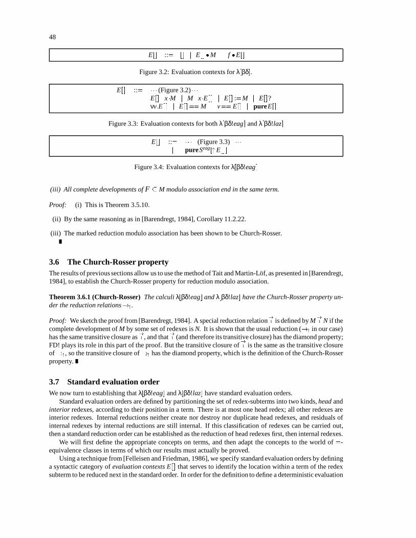
48

E[] ::= [] j E[] M j f E[]

Figure 3.2: Evaluation contexts for λ[βδ].

E[] ::= (Figure 3.2) j E[] .x M j M.x E[ ] j E[] :=M j E[]?j νv:E[ ] j E[] == M j v== E[] j pureE[]

Figure 3.3: Evaluation contexts for both λ[βδ!eag] and λ[βδ!laz]

E[] ::= (Figure 3.3) j pureSeag["E[]]

Figure 3.4: Evaluation contexts for λ[βδ!eag]

(iii) All complete developments of F M modulo association end in the same term.

Proof: (i) This is Theorem 3.5.10.

(ii) By the same reasoning as in [Barendregt, 1984], Corollary 11.2.22.

(iii) The marked reduction modulo association has been shown to be Church-Rosser.

3.6 The Church-Rosser propertyThe results of previous sections allow us to use the method of Tait and Martin-Lof, as presented in [Barendregt,1984], to establish the Church-Rosser property for reduction modulo association.

Theorem 3.6.1 (Church-Rosser) The calculi λ[βδ!eag] and λ[βδ!laz] have the Church-Rosser property un-der the reduction relations!! .

Proof: We sketch the proof from [Barendregt, 1984]. A special reduction relation!

1 is defined by M!

1 N if thecomplete development of M by some set of redexes is N. It is shown that the usual reduction (!! in our case)has the same transitive closure as

!

1 , and that!

1 (and therefore its transitive closure) has the diamond property;FD! plays its role in this part of the proof. But the transitive closure of

!

1 is the same as the transitive closureof!! , so the transitive closure of!! has the diamond property, which is the definition of the Church-Rosserproperty.

3.7 Standard evaluation orderWe now turn to establishing that λ[βδ!eag] and λ[βδ!laz] have standard evaluation orders.

Standard evaluation orders are defined by partitioning the set of redex-subterms into two kinds, head andinterior redexes, according to their position in a term. There is at most one head redex; all other redexes areinterior redexes. Internal reductions neither create nor destroy nor duplicate head redexes, and residuals ofinternal redexes by internal reductions are still internal. If this classification of redexes can be carried out,then a standard reduction order can be established as the reduction of head redexes first, then internal redexes.

We will first define the appropriate concepts on terms, and then adapt the concepts to the world of.=-

equivalence classes in terms of which our results must actually be proved.Using a technique from [Felleisen and Friedman, 1986], we specify standard evaluation orders by defining

a syntactic category of evaluation contexts E[] that serves to identify the location within a term of the redexsubterm to be reduced next in the standard order. In order for the definition to define a deterministic evaluation

49

E[] ::= (Figure 3.3) j pureSlaz["E[]]

Figure 3.5: Evaluation contexts for λ[βδ!laz]

M M1 M2 ) MM1 M2M λx:M1 ) MM1M "M1 ) MM1M M1 .x M2 ) MM1 M2M νv:M1 ) MM1M M1? ) MM1M M1 :=M2 ) MM1 M2M pureM1 ) MM1

M pureSlaz["M1] ) MM1 Slaz[]

Figure 3.6: Subterm ordering for defining the leftmost redex

order, the evaluation contexts for a calculus must have the property that every term has a unique leftmost redexin an evaluation context.

Figures 3.2, 3.3, 3.4, and 3.5 give the definition of evaluation contexts for λ[βδ!eag] and λ[βδ!laz]. Asmight be expected, the only difference between the definition for λ[βδ!eag] in Figure 3.4 and that for λ[βδ!laz]in Figure 3.5 is in the form of the store-context for the evaluation contexts with pure at the root.

The informal intent of these definitions for evaluation contexts is that store-computation proceeds fromleft to right; terms that must be store-variables in order to be useful are forced, but the reduction of others isdeferred. The special forms of evaluation context involving explicit store-contexts are necessary because thecomposition of the other rules will never produce an evaluation context that descends inside a "-expression,hence evaluation specified without the special rules would never force the result of a store-computation andwould thus fail to be a standard order.

The definition in 3.3 requires the proviso that the pattern E[] .x M is given priority over M.x E[ ] in de-termining the head redex. This ordering is formalized as the notion of leftmost evaluation redex. Figure 3.6defines an ordering (read “is to the left of”) of the subterms within a given term. Terms precede their sub-terms in this ordering, the main point being to pin down the relative ordering between subterms for thosesyntactic constructs having more than one. The rule for pureSlaz["M1] in Figure 3.6 takes precedence overthat for pureM1: it is necessary force possible results before allowing store-computation to resume.

We use the ordering to define:

Definition 3.7.1 (Leftmost redex) The leftmost redex subterm of a term M is the least redex subterm of Maccording to the ordering.

The preorder traversal specified in Definition 3.7.1 subsumes the usual definition of ‘leftmost-outermost”.

Definition 3.7.2 (Evaluation, head, internal redexes) (i) A redex ∆ is an evaluation redex of a term M ifM E[∆] for some evaluation context E[].

(ii) The head redex ∆h of a term M is the leftmost evaluation redex of M.

(iii) Any redex subterm of a term M other than a head redex is called an internal redex.

We denote head and internal reductions by affixing the letters h and i respectively to arrows denoting re-ductions.

Lemma 3.7.3 If a term M contains an evaluation redex, it contains a head redex.

Proof: Definition 3.7.2 (i) and (ii) imply this directly.

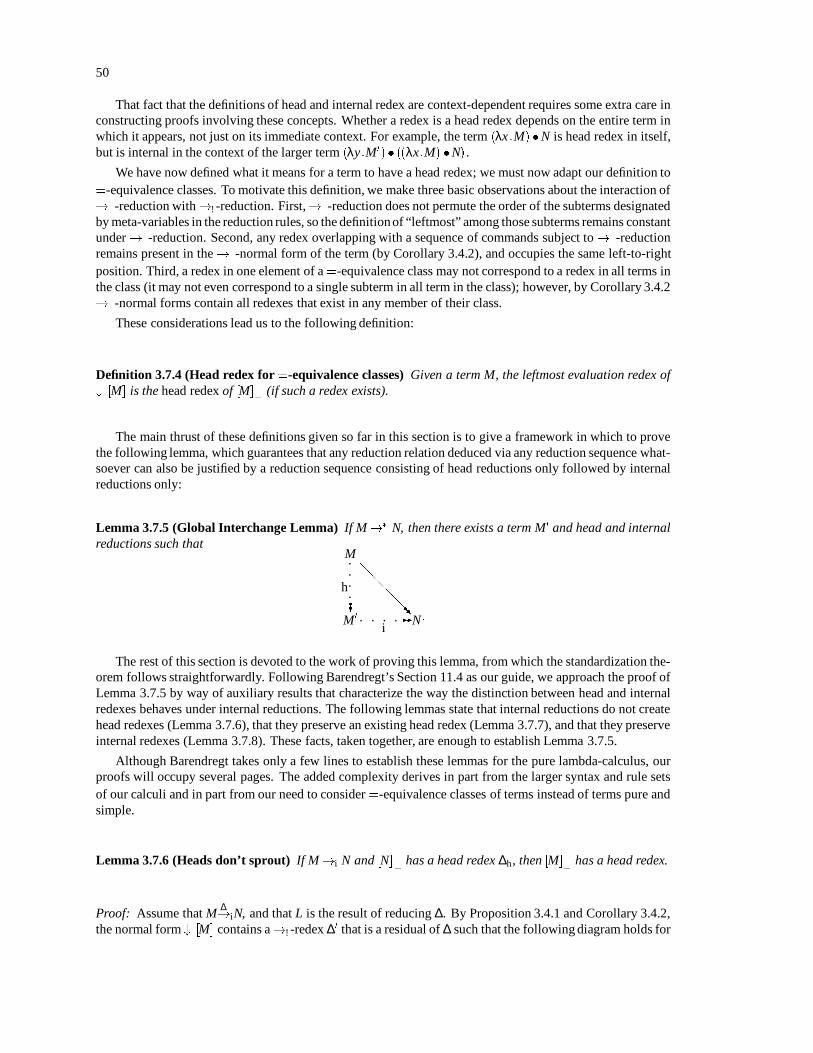
50

That fact that the definitions of head and internal redex are context-dependent requires some extra care inconstructing proofs involving these concepts. Whether a redex is a head redex depends on the entire term inwhich it appears, not just on its immediate context. For example, the term (λx:M) N is head redex in itself,but is internal in the context of the larger term (λy:M0) ((λx:M) N).

We have now defined what it means for a term to have a head redex; we must now adapt our definition to.=-equivalence classes. To motivate this definition, we make three basic observations about the interaction of!. -reduction with!! -reduction. First,!. -reduction does not permute the order of the subterms designatedby meta-variables in the reduction rules, so the definitionof “leftmost” among those subterms remains constantunder!. -reduction. Second, any redex overlapping with a sequence of commands subject to!. -reductionremains present in the!. -normal form of the term (by Corollary 3.4.2), and occupies the same left-to-rightposition. Third, a redex in one element of a .

=-equivalence class may not correspond to a redex in all terms inthe class (it may not even correspond to a single subterm in all term in the class); however, by Corollary 3.4.2!. -normal forms contain all redexes that exist in any member of their class.

These considerations lead us to the following definition:

Definition 3.7.4 (Head redex for .=-equivalence classes) Given a term M, the leftmost evaluation redex of

#. [M] is the head redex of [M] .

=(if such a redex exists).

The main thrust of these definitions given so far in this section is to give a framework in which to provethe following lemma, which guarantees that any reduction relation deduced via any reduction sequence what-soever can also be justified by a reduction sequence consisting of head reductions only followed by internalreductions only:

Lemma 3.7.5 (Global Interchange Lemma) If M! N, then there exists a term M0 and head and internalreductions such that

M

M0 N

@@@@RR

.

.

.

.

.?h

?. . . . .-

i- :

The rest of this section is devoted to the work of proving this lemma, from which the standardization the-orem follows straightforwardly. Following Barendregt’s Section 11.4 as our guide, we approach the proof ofLemma 3.7.5 by way of auxiliary results that characterize the way the distinction between head and internalredexes behaves under internal reductions. The following lemmas state that internal reductions do not createhead redexes (Lemma 3.7.6), that they preserve an existing head redex (Lemma 3.7.7), and that they preserveinternal redexes (Lemma 3.7.8). These facts, taken together, are enough to establish Lemma 3.7.5.

Although Barendregt takes only a few lines to establish these lemmas for the pure lambda-calculus, ourproofs will occupy several pages. The added complexity derives in part from the larger syntax and rule setsof our calculi and in part from our need to consider .

=-equivalence classes of terms instead of terms pure andsimple.

Lemma 3.7.6 (Heads don’t sprout) If M!i N and [N] .

=has a head redex ∆h, then [M] .

=has a head redex.

Proof: Assume that M∆!iN, and that L is the result of reducing ∆. By Proposition 3.4.1 and Corollary 3.4.2,

the normal form #. [M] contains a!! -redex ∆0 that is a residual of ∆ such that the following diagram holds for

51

some term N0 :M

N #. [M]

N0

#. [N]

∆

@@@@R

.

R

@@@R

.

R

@@@R.

R

∆0

:

We will refer to the subterm of N0 that is the result of reducing ∆0 as L0. The diagram permits us to consider∆0 and L0 instead of ∆ and L, since these two terms reflect essentially the same reduction relating the two!. -equivalence classes.

By Definition 3.7.4, ∆h is in head position within #. [N]. The defining reduction rules of!. , assoc andextend, neither create nor destroy syntactic structure but only rearrange it. It is thus reasonable to trace thepieces that make up ∆h backward to find the collection of subterms of N0 that are rearranged into ∆h by the!. -normalization process. Depending on the form of the redex ∆h, this collection (we will denote it by ∆0h eventhough it is not necessarily a single term) may take several forms. If ∆h is a fuse-, bubble-assign-, assign-result-,unit-, or bubble-new-redex, the top-level syntactic constructor of ∆h is .: this case allows ∆0h to consist of sep-arate subterms. If ∆h is a β- or δ-redex ∆0h will consist of a single subterm. If ∆h is a pure-eager- or pure-lazy-redex then ∆0h will likewise consist of a single subterm.

We decompose the proof into three cases depending on the relative positions of L0 and ∆0h. In the first case,L0 and ∆0h are disjoint. In this case, the positions of the subterms will be enough to establish that #. [M] hasan evaluation redex and hence a head redex. In the second case, all the fragments of ∆0h lie within L0. In thiscase also we will be able to reason from the position of the subterms rather than their composition. In the thirdcase, however, in which L0 overlaps ∆0h, we will have to conduct a case analysis on the form of the redex ∆h.

Before we begin the positional analysis, it is important to elaborate on the possible configurations of ∆0h.Consider the maximal command sequence immediately containing ∆h, that is, the largest chain of ν- and .-constructs such that ∆h either overlaps part of the chain or is an element in the chain. Since ∆h is a head redex,there are no evaluation redexes to the left of ∆h in this maximal chain, a fact that is reflected in the collectionof subterms ∆0h because!. -reduction preserves the order of subterms. In more formal terms, #. [N] must havethe form E1[Slaz [E2 [∆h ]]], where there is no evaluation redex in Slaz[], and the (lazy) store-context Slaz[] is thelongest such sequence immediately surrounding ∆h.

Case 1: L0 and ∆0h are disjoint. In this case, no part of the result of reducing ∆ is assembled into ∆h, yet ∆his head redex in #. [N]. We argue that the antecedent of ∆h must then exist and be the head redex in#. [M] (and this must be, by Definition 3.7.4, the head redex of [M] .

=).

The existence of the antecedent of ∆0h as a redex within #. [M] follows from two observations. First,since L0 is disjoint from ∆0h, ∆0h is an unaltered copy of a subterm of #. [M] disjoint from ∆0. Second,since #. [M] is in!. -normal form, so are all its subterms, including ∆0h. Hence ∆0h is really the sameas the redex ∆h—it is not possible in this case for ∆0h to be a set of fragments to be assembled into ∆hby!. .

We next note that L0 cannot be in an evaluation context to the left of ∆0h, because this would make ∆0a head redex, whereas it is assumed in the statement of the lemma to be internal. Hence the contextin which ∆0 occurs must be either a non-evaluation context or an evaluation context to the right of theantecedent of ∆0h. If the latter case applies, the mere existence of an evaluation redex establishes theexistence of a head redex (Lemma 3.7.3). We are thus left to consider the cases in which ∆0 occupiesa non-evaluation context.

52

Since ∆0 must be disjoint from the antecedent of ∆0h (which is ∆h, as we showed just above), there mustbe some multiple-subterm syntax constructor that forms the least common ancestor of the two terms.Furthermore, since ∆h lies within an evaluation context in the whole term (since the only change oc-curs within∆), this common ancestor must itself be in an evaluation context and ∆h must be in a nestedevaluation context starting at the common ancestor.

The following list enumerates all the ways in which this situation can arise.

(1) E1[E2 [∆h ]C[∆0 ]],(2) E1[E2 [∆h ] :=C[∆0 ]],(3) E1[E2 [∆h ].x C[∆0 ]],(4) E1[C[∆0 ].x E2 [∆h ]], where C[ ] is not an evaluation context,

(5) E1[pure Seag[" E2[∆h ]]], where ∆0 Seag[]. (This case applies to λ[βδ!eag]),

(6) E1[pure Slaz["E2[∆h ]]], where ∆0 Slaz[]. (This case applies to λ[βδ!laz]).

In each of these cases, ∆h is an evaluation redex of #. [M]; hence #. [M] must have a head redex.

Case 2: ∆0h L0.

Since ∆0h may not be a single subterm, the assertion characterizing this case should be understood tomean that all the components of ∆0h are subterms of L0, which in turn implies that all the componentsof ∆0h arise from the reduction of ∆0. More formally, if ∆0 appears in a general term context C1 [], i.e.#. [M] C1 [∆0 ], then N0 C1 [L0 ] and N0 !. C1 [C2 [∆h ]] for some general term context C2 [ ]. Since∆h is known to be a head redex, the enclosing context C1 [C2 []] must be an evaluation context. Sinceevaluation contexts are inductively defined in such a way that any prefix of an evaluation context isalso an evaluation context, the context C1 [] must be an evaluation context. We have now shown Mto have at least one evaluation redex, so by Lemma 3.7.3 it must have a head redex.

Case 3: L0 ∆0h.

In case ∆0h consists of more than one term, we interpret L0 ∆0h to mean that there is some term Q inthe set composing ∆0h for which L0 Q. For an example of this possibility, suppose that N0 has theform (("N01).x N0

2).y N0

3 , where L0 is the subterm ("N01 ).x N0

2 . The!. -normal form #. [N0 ] thenhas the form ("N01 ).x #. [N0

2 .y N0

2 ], where ∆h consists of the entire term #. [N0 ]. The subterm L0 isnot a subterm of this normal form. In the subcases that follow, we must account for this possibilitythat L0 may be fragmented into more than one different subterm of ∆h.

In this case the reduction must have the general form M0 E[ bM]∆0

!E[∆0h ] for some evaluation contextE[] and subterm bM with ∆0 bM. We now carry out a case analysis according to the form of the redex∆h #. [N0 ], and show that for each form, the antecedent bMM0 of ∆0h has an evaluation redex (andhence, by Lemma 3.7.3, a head redex).

For each case, we list the possible forms of bM and the correspondingevaluation redex whose existencewe must establish. The notation C+ [∆] refers to the redex ∆ in a non-empty context.

(a) β: ∆h (λx:N1 )N2 .Since!. cannot shuffle terms whose syntactic constructor is , the antecedent ∆0h of ∆h withinN0 has the same form, with some!. -conversion possible within the subterms. So if we let ∆0h (λx:N0

1) N20, and if we consider all the ways that this subterm can be produced from an an-

tecedent bM, we obtain the following table which displays the evaluation redex whose existenceis implied:bM : eval. redex:∆0 N02 ∆0

(λx:C[∆0 ])N02 bM(λx:N0

1 )C[∆0 ] bM

53

(b) δ: ∆h f VThis case is subject to the same reasoning concerning the form of ∆0h as the case of β and givesus the following table for establishing the existence of an evaluation redex in bM:bM : eval. redex:∆0 V0 ∆0f ∆0 ∆0f (C[∆0 ] ) ∆0

f (cn C[∆0 ] ) bMf (λx:C[∆0 ]) bM

(c) unit: ∆h "N1 .x N2

For this and other forms of redex whose root syntactic constructor is . we need to consider care-fully the effect of the!. -reduction leading from ∆0h to ∆h. If we suppose that ∆h is the result of aassoc- or extend-reduction involving the occurrence of . that forms the root of ∆h, we see that the(possibly multiple) terms making up ∆0h must include exactly one of the form "N01 .x N0

2 , whereN02 might be a shorter command sequence (in terms of number of occurrences of . on its spine)than N2 . The other terms in ∆0h are those tacked onto N02 by assoc- or extend-reductions. We callthe former kind essential and the latter trivial.If L0 is a subterm of the essential element of ∆0h, we can deduce the following table giving therequired evaluation redexes:bM : eval. redex:∆0 .x N0

2 ∆0

"C[∆0 ].x N0

2bM

"N01 .x C[∆0 ] bM

If, on the other hand, L0 is a subterm of a trivial element of ∆0h, then the entire antecedent bM is anevaluation redex.

(d) fuse: ∆h v :=N1 ; v? .x N2

The considerations and terminology given under the case for unit apply here as well. If L0 is asubterm of the essential element of ∆0h, then we construct the following table of cases:bM : eval. redex:∆0; v? .x N0

2 ∆0

v :=C[∆0 ]; v? .x N0

2bM

∆0 :=N01 ; v? .x N0

2 ∆0v :=N01 ; ∆0 ∆0v :=N01 ; ∆0 .x N0

2 ∆0v :=N01 ; ∆0?.x N0

2 ∆0

v :=N01 ; v? .x C[∆0 ] bM

If, on the other hand, L0 is a subterm of a trivial element of ∆0h, then bM itself must be an evaluationredex.

(e) bubble-assign: ∆h v :=N1 ; w?.x N2

We invoke the same reasoning and terminology as in the previous two cases. If L0 is a subtermof an essential element of ∆0h, then we construct the tablebM : eval. redex:∆0; w?.x N0

2 ∆0

v :=C[∆0 ]; w?.x N0

2bM

∆0 :=N01 ; w?.x N0

2 ∆0v :=N01 ; ∆0 ∆0v :=N01 ; ∆0 .x N0

2 ∆0v :=N01 ; ∆0?.x N0

2 ∆0

v :=N; ∆.x C[∆0 ] bM

.

54

If, on the other hand, L0 is a subterm of a trivial element of ∆0h, then bM itself is the evaluationredex we seek.

(f) assign-result: ∆h v :=N1 .x N2 ;x 2 fv N2

The usual reasoning for redexes formed by . applies once more. If L0 is a subterm of an essentialelement of ∆0h we can deduce the information in the following table.bM : eval. redex:∆0 .x N0

2 ∆0∆0 :=N01 .x N0

2 ∆0

v :=C[∆0 ].x N0

2bM

v :=N01 .x C[∆0 ] bM

If, on the other hand, L0 is a subterm of a trivial element of ∆0h, then bM itself is the evaluationredex we seek.

(g) bubble-new: ∆h νv:w? .x N1

The usual reasoning for redexes formed by . applies once more. If L0 is a subterm of an essentialelement of ∆0h we can deduce the information in the following table.bM : eval. redex:νv:∆0 ∆0νv:∆0 .x N0

1 ∆0νv:∆0 ?.x N0

1 ∆0

νv:w? .x C[∆0 ] bM

If, on the other hand, L0 is a subterm of a trivial element of ∆0h, then the entire antecedent bM is theevaluation redex we seek.

(h) pure-eager: ∆h pureSeag["V]

This case applies in the calculus λ[βδ!eag].

Since the root syntactic constructor, pure, of this redex is not subject to!. -reductions, ∆0h mustalso be a pure construct, perhaps with some associative rearrangement of the store-context. Wesubdivide this case according the the position of L0 as a subterm of ∆0h. We denote the antecedentof V in ∆0h by V0 .

(1) L0 disjoint from V0 .In this case, bM pureSeag

1 [C1 [∆0 ].x Seag2 ["V]] for some store contexts Seag

1 [] and Seag2 [] and

general term context C1 []. Since the whole body of the pure expression must associate intoa pure-redex, the subterm C1 [L0 ] must actually (associate to) a fragment of an eager store-context, that is, it must consist of a sequence of ν and assignment commands. We now sub-divide the possible locations into cases yet again:

(a) L0 encompasses one or more command.In this case the redex ∆0 #. [M] that reduces to L0 occupies the prefix of a commandsequence. This is an evaluation context.

(b) L0 lies completely within a command.The following table gives all the ways this can happen, along with the evaluation redexwhose existence is required. We note that it is not possible in this case for further!. -reduction of the main command sequence to be required, since ∆0 occurs in a term thatis already in!. -normal form.bM : eval. redex:

pureSeag1 [∆0 :=N02 .x Seag

2 ["V]] ∆0

pureSeag1 [N0

1 :=∆0 .x Seag2 ["V]] bM

(2) L0 V0 .Recalling that pureSeag[" []] is an evaluation context, we construct the following table ofpossibilities:

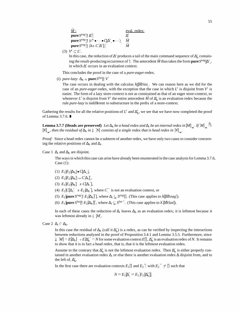
55

bM : eval. redex:pureSeag["∆0] ∆0

pureSeag[" (cn C[∆0 ] )] bMpureSeag[" (λx:C[∆0 ])] bM

(3) V0 L0.In this case, the reduction of ∆0 produces a tail of the main command sequence of ∆0h contain-ing the result-producingoccurrence of ". The antecedent bM thus takes the form pureSeag[∆0 ],in which ∆0 occurs in an evaluation context.

This concludes the proof in the case of a pure-eager-redex.

(i) pure-lazy: ∆h pureSlaz["V]

The case occurs in dealing with the calculus λ[βδ!laz]. We can reason here as we did for thecase of an pure-eager-redex, with the exception that the case in which L0 is disjoint from V0 iseasier. The form of a lazy store-context is not as constrained as that of an eager store-context, sowhenever L0 is disjoint from V0 the entire antecedent bM of ∆0h is an evaluation redex because therule pure-lazy is indifferent to substructure in the prefix of a store-context.

Gathering the results for all the relative positions of L0 and ∆0h, we see that we have now completed the proofof Lemma 3.7.6.

Lemma 3.7.7 (Heads are preserved) Let ∆h be a head redex and ∆i be an internal redex in [M] .=

. If [M] .=

∆i!

[N] .

=, then the residual of ∆h in #. [N] consists of a single redex that is head redex in [N] .

=.

Proof: Since a head redex cannot be a subterm of another redex, we have only two cases to consider concern-ing the relative positions of ∆h and ∆i.

Case 1 ∆i and ∆h are disjoint.

The ways in which this case can arise have already been enumerated in the case analysis for Lemma 3.7.6,Case (1):

(1) E1[E2 [∆h ]C[∆i ]],

(2) E1[E2 [∆h ] :=C[∆i ]],

(3) E1[E2 [∆h ].x C[∆i ]],

(4) E1[C[∆i ].x E2 [∆h ]], where C[ ] is not an evaluation context, or

(5) E1[pure Seag["E2[∆h ]]], where ∆i Seag[]. (This case applies to λ[βδ!eag]).

(6) E1[pure Slaz["E2[∆h ]]], where ∆i Slaz[]. (This case applies to λ[βδ!laz]).

In each of these cases the reduction of ∆i leaves ∆h as an evaluation redex; it is leftmost because itwas leftmost already in #. [M].

Case 2 ∆i ∆h.

In this case the residual of ∆h (call it ∆0h) is a redex, as can be verified by inspecting the interactionsbetween reductions analyzed in the proof of Proposition 3.4.1 and Lemma 3.5.5. Furthermore, since#. [M]E[∆h ]!E[∆0h ]N for some evaluation context E[], ∆0h is an evaluation redex of N. It remainsto show that it is in fact a head redex, that is, that it is the leftmost evaluation redex.

Assume to the contrary that ∆0h is not the leftmost evaluation redex. Then ∆0h is either properly con-tained in another evaluation redex ∆, or else there is another evaluation redex ∆ disjoint from, and tothe left of, ∆0h.

In the first case there are evaluation contexts E1[] and E2[] with E2[] 6 [] such that

N E1[∆] E1[E2 [∆0h ]]:

56

Since ∆i ∆h, there is a nonempty general term context C[ ] such that

#. [M] E1[E2 [∆h ]] E1[E2 [C[∆i ]]];

and thus (carrying out the reduction)

N E1[E2 [C[∆0i ]]];

where ∆0i is the residual of ∆i. Now the question is, how did ∆ arise? The reduction of ∆i as a subterm of∆h could not have created a redex outside of ∆h, as an inspection of the set of reduction rules will show.Therefore, the antecedent of ∆ existed as an evaluation redex in #. [M], contradicting the assumptionthat its proper subterm ∆h was the head redex.

In the second case, we can find evaluation contexts E1[], E2[], E3[] such that N is one of the following:

(1) E1[E2 [∆] E3[∆0h ]]

(2) E1[E3 [∆0h ] :=E2[∆]]

(3) E1[v := E2[∆] .x E3 [∆0h ]].

Hence, #. [M] is one of the following:

(1) E1[E2 [∆] E3[∆h ]]

(2) E1[E3 [∆h ] :=E2[∆]]

(3) E1[v := E2[∆] .x E3 [∆h ]].

In each case, ∆ is an evaluation redex to the left of ∆h, contradicting the assumption that ∆h is the headredex.

Lemma 3.7.8 (Internals are preserved) For any term M in!. -normal form and internal redex ∆i M, forany internal reduction M!i N, all residuals of ∆i are internal redexes of #. [N].

Proof: Assume, to the contrary, that there is a residual ∆ of ∆i that is a head redex in N. By Lemma 3.7.6, Mhas a head redex ∆h. By Lemma 3.7.7, ∆ is the residual of ∆h. This contradicts the assumption that ∆ was aresidual of the internal redex ∆i.

We have now established the properties of our calculi needed to prove the standardization theorem by thetechniques (attributed to Mitschke) of [Barendregt, 1984], Section 11.4. The main thrust of the cited work is toprove the result we have stated in Lemma 3.7.5. Knowing that head and internal reductions can be interchangelets us single out the standard reduction sequences as those that proceed in an orderly fashion from left to right.

Definition 3.7.9 (Standard reduction sequence) A sequence of reductions M0∆0!M1

∆1!

∆n1! Mn is a stan-

dard reduction sequence if, for all i < j, ∆ j is not a residual of a redex to the left of ∆i.

Theorem 3.7.10 (Standardization) If M! N, then there exists a standard reduction sequence from M toN.

The following related result on the computation of answer terms is used in the proof of Theorem 5.1.7. Thetheorem says that answer terms are built in a top-down order, outermost constructors first, then components.

Definition 3.7.11 (Top-down reduction to an answer) A reduction sequence ending in an answer A is top-down if either it consists entirely of head reductions, or consists of a head reduction sequence ending in a termcn M1 Mk;k n, followed by a top-down reduction sequence for M1, and so on through Mk.

57

In Definition 3.7.11 the head-ness of the subsequences is interpreted with respect to the subterm in ques-tion.

Theorem 3.7.12 (Standard reduction to an answer) If M! A, where A is an answer, then the standardreduction sequence from M to A is top-down.

Proof: The proof is by induction on the struction of the answer term A. The base cases are A c0 and A f ,both of which are terms with no internal structure. In these cases the last reduction of the sequence must haveproduced the answer term by reducing the entire term. This is a head reduction, so there is no segment of thereduction sequence using internal reductions. The reduction sequence is thus top-down.

Now assume that A cn A1 Ak;0 < k n;. Again consider the last reduction that produced A: thisreduction must have either involved the entire term as redex, producing all of A, or else it resulted in one of thesubterms Ai. In the former case the last reduction is a head reduction, and hence all its predecessors are also;thus the reduction sequence is top-down. In the latter case the induction hypothesis applies to show that thereduction sequence producingAi is top-down. Furthermore, since the reduction is standard, the subterms to theleft of Ai must have been produced earlier in the reduction sequence, and the subterms to the right of Ai mustalready be answers. We can thus apply the induction hypothesis to the term cn A1 Ai1 . Putting all thetop-down reduction sequences together in the order we have deduced yields a top-down reduction sequencefor A.

3.8 Relating properties of!! to properties of!

We have now proved the Church-Rosser theorem and standardization theorem for!. on.=-equivalence classes.

In this section we translate these results back into!, which is the reduction relation we actually intend to use.

Theorem 3.8.1 (Church-Rosser) The reduction relation! on λ[βδ!eag] and λ[βδ!laz] is Church-Rosser.

Proof: Suppose we are given the top half of a Church-Rosser diagram under reduction!:

M

M1 M2

!

@@@@@@R

!

R: (3.3)

Each of the given reduction sequences consists of some interleaving of!. -reductions and!! -reductions onterms. Passing to .

=-equivalence classes, the!. -steps collapse (since they stay within the same equivalenceclass), and the!! -steps on terms become!! -steps on equivalence classes:

[M] .=

[M1 ] .= [M2 ] .=

!!

@@@@@@R

!!

R:

58

Since!! is Church-Rosser on equivalence classes (Theorem 3.6.1), we can complete the diamond to obtaina term N0 such that the diagram

[M] .=

[M1 ] .= [M2 ] .=

N0

!!

@@@@@@R

!!

R

..

..

..

..

.R

!!

R

..

..

..

..

.

!!

: (3.4)

commutes. We would now like to use this diagram for !! on equivalence classes to help us complete thediagram 3.3. The first step in doing this is to note that each of the terms M1 and M2 can be normalized withrespect to!. while staying within the same .

=-equivalence class, giving us (so far), the diagram

M

M1

#. [M1 ]

M2

#. [M2 ]

!

?!.

?

@@@@@@R

!

R

?!.

?

:

The next step is to use the information given us by diagram 3.4. This diagram assures us that, somewhere ineach of the equivalence classes [M1 ] .= and [M2 ] .= there is a term that reduces via!! on terms to some termin the common equivalence class N0 . However, if such reductions exist, then by Corollary 3.4.2 we can beassured that they exist starting at the normal forms #. [M1 ] and #. [M2 ]. Furthermore, since these reductionsland in the same equivalence class N0 , the terms in which the end must be convertible via!. . Thus we have

M

M1

#. [M1 ]

M0

1

M2

#. [M2 ]

M0

2.=

!

?!.

?

?!!

@@@@@@R

!

R

?!.

?

?!!

:

59

But now, since!. is Church-Rosser (Theorem 3.3.3), the convertible terms M0

1 and M0

2 must have a commonreduct M0. This fact allows us to establish the diagram

M

M1

#. [M1 ]

M0

1

M2

#. [M2 ]

M0

2.=

M0

!

?!.

?

?!!

@@@@@@R

!.

R

@@@@@@R

!

R

?!.

?

?!!

!.

;

which is a complete diamond for!. We have thus shown that! is Church-Rosser.

We now turn to the question of deriving a standardization result for λ[βδ!eag] and λ[βδ!laz] from the re-sults we have for the reduction!! on .

=-equivalence classes. We lift sequences of!! -reductions to sequencesof!-reductions by reducing to!. -normal form before each!! -step. We take a standard reduction sequenceunder! to be one thus derived from a standard reduction sequence under!! . The question now is whether ithas the same nice characterization in terms of evaluation contexts as the original reduction sequence. We notethat the reduction order so defined is certainly deterministic: Proposition 3.3.8 and Theorem 3.7.10 combineto show this. Since head redexes are defined in terms of!. -normal forms, the derived!-reduction selectsthe same redexes as the original!! -reduction sequence. Furthermore, by the remark in the proof of Propo-sition 3.3.8, we can choose the same definition of evaluation contexts to define the reduction order for the!. -steps as we do in defining the standard order for!! -reductions. Collecting all these remarks, we haveestablished that the evaluation contexts defined for Definition 3.7.1 yield a standard order of evaluation for!.

3.9 Chapter summaryThis chapter has established the credentials of λ[βδ!eag] and λ[βδ!laz] as a foundation for programming-language design on the same basis as the pure lambda-calculus. We have introduced the derived reductionrelation of reduction modulo association and shown it to be Church-Rosser and to possess a standard evalua-tion order, and we have used these results to establish the same properties of the original reduction relations. Inthe remainder of the dissertation we will thus have no need to refer to the factored reduction relation employedas a proof technique in this chapter.

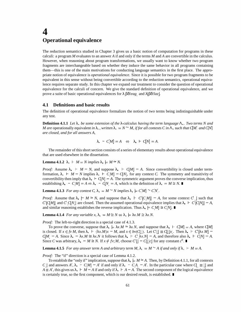
4Operational equivalence

The reduction semantics studied in Chapter 3 gives us a basic notion of computation for programs in thesecalculi: a program M evaluates to an answer A if and only if the terms M and A are convertible in the calculus.However, when reasoning about program transformations, we usually want to know whether two programfragments are interchangeable based on whether they induce the same behavior in all programs containingthem—this is one of the main motivations for conducting language semantics in the first place. The appro-priate notion of equivalence is operational equivalence. Since it is possible for two program fragments to beequivalent in this sense without being convertible according to the reduction semantics, operational equiva-lence requires separate study. In this chapter we expand our treatment to consider the question of operationalequivalence for the calculi of concern. We give the standard definition of operational equivalence, and weprove a suite of basic operational equivalences for λ[βδ!eag] and λ[βδ!laz].

4.1 Definitions and basic resultsThe definition of operational equivalence formalizes the notion of two terms being indistinguishable underany test.

Definition 4.1.1 Let λ be some extension of the λ-calculus having the term language Λ. Two terms N andM are operationally equivalent in λ , written λ j= N = M, if for all contexts C in Λ such that C[M] and C[N]are closed, and for all answers A,

λ ` C[M] = A , λ ` C[N] = A:

The remainder of this short section consists of a series of elementary results about operational equivalencethat are used elsewhere in the dissertation.

Lemma 4.1.2 λ ` M = N implies λ j= M= N.

Proof: Assume λ ` M = N, and suppose λ ` C[M] = A. Since convertibility is closed under term-formation, λ ` M = N implies λ ` C[M] = C[N], for any context C. The symmetry and transitivity ofconvertibility then imply that λ ` C[N] = A. The symmetric argument proves the converse implication, thusestablishing λ ` C[M] = A, λ ` C[N] = A, which is the definition of λ j= M= N.

Lemma 4.1.3 For any context C, λ j= M = N implies λ j= C[M] = C[N].

Proof: Assume that λ j= M = N, and suppose that λ ` C0 [C[M]] = A, for some context C0 [ ] such thatC0 [C[M]] and C0 [C[N]] are closed. Then the assumed operational equivalence implies that λ ` C0 [C[N]] = A,and similar reasoning establishes the reverse implication. Thus λ j= C[M] = C[N].

Lemma 4.1.4 For any variable x, λ j= M= N, λ j= λx:M = λx:N.

Proof: The left-to-right direction is a special case of 4.1.3.To prove the converse, suppose that λ j= λx:M = λx:N, and suppose that λ ` C[M] = A, where C[M]

is closed. If x 2 fv M, then λ ` (λx:M)x = M, and x 2 bv(C[ ]). Let C0 [] C[[ ]x]. Then λ ` C0 [λx:M] =C[M] = A. Since λ j= λx:M = λx:N it follows that λ ` C0 [λx:N] = A, and therefore also λ ` C[N] = A.Since C was arbitrary, λ j= M = N. If x 62 fv; M, choose C0 [] = C[[ ]c] for any constant c0.

Lemma 4.1.5 For any answer term A and arbitrary term M, λ j= M= A if and only if λ ` M = A.

Proof: The “if” direction is a special case of Lemma 4.1.2.To establish the “only if” implication, suppose that λ j= M= A. Then, by Definition 4.1.1, for all contexts

C[ ] and answers A0, λ ` C[M] = A0 if and only if λ ` C[A] = A0. In the particular case where C[ ] [] andA A0, this gives us λ ` M = A if and only if λ ` A= A. The second component of the logical equivalenceis certainly true, so the first component, which is our desired result, is established.

61

62

4.2 Some operational equivalences in λ[βδ!eag] and λ[βδ!laz]

In this section we prove a small collection of operational equivalences that hold in the calculi λ[βδ!eag] andλ[βδ!laz]. These equivalences are selected to correspond to frequently-used informal properties of program-ming with store-variables and assignment.

Proposition 4.2.1 The following are operational equivalences in λ[βδ!eag] and λ[βδ!laz]:

(1) v?.x w? .y M = w?.y v? .x M

(2) v :=N; w :=N0 ; M = w :=N0 ; v :=N; M; (v 6= w)

(3) νv:w := N; M = w :=N; νv:M; (v 6= w;v 62 fsvN)

(4) νv:νw:M = νw:νv:M

(5) v :=N; v :=N0 ; M = v :=N0 ; M

(6) P .x " x = P

Proposition 4.2.2 The following is an operational equivalence in the calculus λ[βδ!eag] if there is no assign-ment in Seag[] to any store-variable v 2 fv P.

(7) Seag[P] = P; (fv Seag[P] = fv P)

We will prove these operational equivalances immediately below, but first we describe what they mean interms of informal programming concepts.

Equivalence (1) says that store-variable lookups commute. Equivalences (2), (3) and (4) say that assign-ments and store-variable declarations commute with themselves and with each other. Equivalence (5) saysthat if a variable is written twice in a row, the second assigned value is the one that counts.

Equivalence (6) is the right-identity law for monads. Although our reduction semantics does not axioma-tize this law, we recover it in the theory of operational equivalence.

Equivalence (7) represents “garbage collection”: it says that a store-context Seag[] of an expression Seag[P]can be dropped if no variable written or in Seag[] is used in P. Note that, using the “bubble” conversion laws andthe commutative laws (2), (3) and (4), garbage can always be moved to an eager store-prefix. This operationalequivalence is stated only for λ[βδ!eag] because there is no way of defining the set of store-variables assignedin a lazy store-context Slaz[]—not all assignment commands in such a store-context need be apparent statically.

We should note that none of these proposed operational equivalences is provable by conversion. If weconsider the meta-variables as ordinary variables there is not a single redex on either side of any of the equiv-alences, so the two sides are actually distinct normal forms and hence not interconvertible.

Proof technique

The definition of operational equivalence demands that we prove statements that are quantified over all con-texts in each calculus; the statements themselves are quantified over all answer-producing reductions. It is notimmediately clear how to proceed in the face of these complex requirements, but we have available to us aproof technique developed by Odersky [Odersky, 1993a] to reduce this burden of proof. This technique re-quires us only to prove certain properties of the interaction between the proposed operational equivalence andthe reduction rules of the calculus. We give this technique in outline before we proceed to use it in the proofsbelow.

Oderksy’s technique requires that, for each proof, we construct a collection of symmetric rewrite rules thatdefine a relation, similarity, intended to characterize the operational equivalence to be proved. In our presentproposition, this collection will always consist of a single rule, which will be the operational equivalence asstated. We must then show that, in all cases in which the similarity rules have a critical overlap (see Section 3.2)with the reduction rules of the calculus, there exists a parallel application of (already-established) operationalequivalences to the similar term that yields a term similar to the result of the reduction.

The main proof requirements for each operational equivalence are explained in relation to the followingdiagram:

63

R R0 R01

R00 R001

-h

. . . . . . . . .-h

1

. . . . . . . . . . . . . . . . . .-=

.

.

.

.

.

.

.

.

1

In this diagram 1 is the parallel similarity derived from . In our proofs it will suffice to think of 1as being the union of the relation with syntactic identity. The h labeling the arrow means that the corre-sponding reduction is a head reduction.

For each proof below, we will give concrete meta-terms and reductions to instantiate this diagram.

Applying the proof technique requires in addition that we establish certain highly technical conditions.First, we must verify that the evaluation contexts of λ[βδ!eag] and λ[βδ!laz] are downward closed, that is, thatE = C1 C2 implies that C2 is itself an evaluation context. This is obvious from inspection of the definition ofevaluation contexts in Figures 3.2, 3.3, 3.4, and 3.5. Second, we must establish, for each similarity relationwe introduce, that the relation preserves evaluation contexts and is answer-preserving.

Preservation of evaluation contexts means that substituting instances of a similarity rule for a metavariablein an non-evaluation context cannot transform that context into an evaluation context. Put another way, therequirement is that collapsing similarity-rule instances to a single metavariable cannot destroy an evaluationcontext. It is easy to see that the definitions of the evaulation contexts for λ[βδ!eag] and λ[βδ!laz] given inFigures 3.2, 3.3, 3.4, and 3.5 prevent this possibility. The point to note is that substructure of a rule defining E[]is always a metavariable or the recursive reference to E[] . Thus any collpase of a similarity-rule instance mustoccur either within a metavariable of an E[] -rule, because the context hole cannot occur within a similarityrule instance in the technical formulation of [Odersky, 1993a].

An answer-preserving relation satisfies M A)M! A; this is easily seen to be true for all our proposedsimilarity relations (most often vacuously, since our similarity patterns do not match answer terms), so we willomit further mention of this issue.

Proof: We now proceed to prove each of the proposed operational equivalences. Although the bottom edgeof the diagram can be any operational equivalence, in many cases the operational equivalence is easily estab-lished by exhibiting a conversion. We only remark on the exceptions to this observation.

For each of the operational equivalences to be proved, we supply the needed similarity relation in the formof a set of rewrite rules and then give the data needed to instantiate the diagram above. We label the proofs ofthe parts of Propositions 4.2.1 and 4.2.2 by number.

(1) We adopt the similarity relation implied by S = fv? .x w? .y M w?.y v? .x Mg.

The rules in S do not overlap with any of the productions defining evaluation contexts in Figures 3.2, 3.3,and 3.4. Hence, preserves evaluation contexts.

We now enumerate the various ways in which can intefere with!; for each case, we show how to in-stantiate the diagram so as to prove that the compatible equivalence closure of is an operational equivalence.In this instance the cases are distinguished by which store-variables are identical in the various terms.

64

Case 1.1:

R u :=N; v? .x w? .y M; (u 6 v;u 6 w;v 6 w)R00 u :=N; w?.y v? .x MR0 v? .x u := N; w?.y MR01 v? .x w? .y u := N; MR001 w?.y v? .x u := N; M

R !bubble-assign R0

R0 !bubble-assign R01R00 !bubble-assign w?.y u := N; v? .x M

!bubble-assign R001

Case 1.2:

R w :=N; v?.x w? .y M; (u 6 v;v 6 w)R00 w :=N; w?.y v? .x MR0 v?.x w := N; w?.y M

R01 R001 v?.x w := N; [N=y] M

R !bubble-assign R0

R0 !fuse R01R00 !fuse w :=N; [N=y] (v? .x M)

w :=N; v?.x [N=y] M!bubble-assign R001

Case 1.3:R v :=N; v? .x w? .y M; (v 6 w)

R00 v :=N; w?.y v? .x MR0 v :=N; [N=x] (w? .y M)

v :=N; w?.y [N=x]MR01 R001 R0

R !fuse R0

R00 !bubble-assign w?.y v := N; v? .x M

!fuse R001

Case 1.4:R u :=N; v? .x v? .y M; (u 6 v)

R0 v?.x u := N; v? .y MR00 u :=N; v? .y v? .x MR01 v?.x v? .y u := N; MR001 v?.y v? .x u := N; M

R !bubble-assign R0

R0 !bubble-assign R01R00 !bubble-assign v?.y u := N; v?.x M

!bubble-assign R001

65

Case 1.5:R v :=N; v? .x v? .y M

R0 v :=N; [N=x] v? .y M v :=N; v? .y [N=x]M

R00 RR01 R0

R001 R01

R !fuse R0

R0 R01R00 !fuse R001

For the remaining operational equivalences, we give only the basic data needed to complete the diagram.

(2) S = fv := N; w :=N0 ; M w :=N0 ; v :=N; Mg; (v 6 w).

Case 2.1:

R v :=N; w :=N0 ; w?.x M0 ; (v 6 w)R0 v :=N; w :=N0 ; [N0=x]MR01 R0

R00 w :=N0 ; v :=N; w?.x M0

R001 w :=N0 ; v :=N; [N0=x]M0

R !fuse R0

R00 !bubble-assign w :=N0 ; w?.x v := N; M0; (since x 62 fv N)

!fuse w :=N0 ; [N0=x] (v := N; M0)

R001

Case 2.2:R v :=N; w :=N0 ; v? .x M ; (v 6 w)R0 v :=N; v?.x w := N0 ; M; (x 62 fv N0 )R00 w :=N0 ; v :=N; v? .x MR01 v :=N; w :=N0 ; [N=x]MR001 w :=N0 ; v :=N; [N=x]M

R !bubble-assign R0

R0 !fuse v :=N; [N=x] (w := N0 ; M)

R01; (since x 62 fv N0 )R00 !fuse R001

Case 2.3:R v :=N; w :=N0 ; u?.x M ; (u 6 w;u 6 v)

R0 v :=N; u?.x w := N0 ; MR00 w :=N0 ; v :=N; u?.x MR01 u?.x v := N; w :=N0 ; MR001 u?.x w := N0 ; v :=N; M

R !bubble-assign R0

R0 !bubble-assign R01R00 !bubble-assign w :=N0 ; u?.x v := N; M

!bubble-assign R001

(3) S = fνv:w := N; M w :=N; νv:Mjv 6 w;v 62 fv Ng

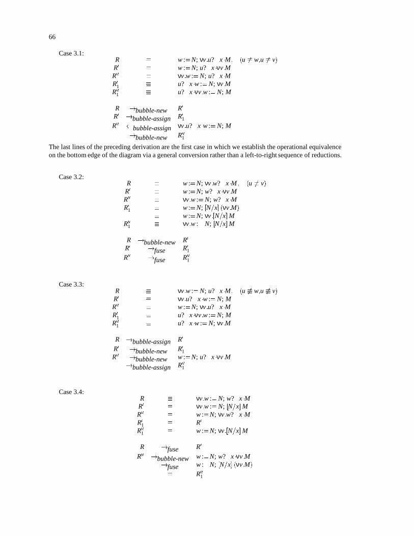
66

Case 3.1:R w :=N; νv:u? .x M; (u 6 w;u 6 v)R0 w :=N; u?.x νv:MR00 νv:w := N; u?.x MR01 u?.x w := N; νv:MR001 u?.x νv:w := N; M

R !bubble-new R0

R0 !bubble-assign R01R00 bubble-assign νv:u? .x w := N; M

!bubble-new R001

The last lines of the preceding derivation are the first case in which we establish the operational equivalenceon the bottom edge of the diagram via a general conversion rather than a left-to-right sequence of reductions.

Case 3.2:R w :=N; νv:w? .x M ; (u 6 v)

R0 w :=N; w?.x νv:MR00 νv:w := N; w?.x MR01 w :=N; [N=x] (νv:M)

w :=N; νv:[N=x]MR001 νv:w := N; [N=x]M

R !bubble-new R0

R0 !fuse R01R00 !fuse R001

Case 3.3:R νv:w := N; u?.x M; (u 6 w;u 6 v)R0 νv:u? .x w := N; MR00 w :=N; νv:u? .x MR01 u?.x νv:w := N; MR001 u?.x w := N; νv:M

R !bubble-assign R0

R0 !bubble-new R01R00 !bubble-new w :=N; u?.x νv:M

!bubble-assign R001

Case 3.4:R νv:w := N; w?.x M

R0 νv:w := N; [N=x]MR00 w :=N; νv:w? .x MR01 R0

R001 w :=N; νv:[N=x]M

R !fuse R0

R00 !bubble-new w :=N; w?.x νv:M!fuse w :=N; [N=x] (νv:M)

R001

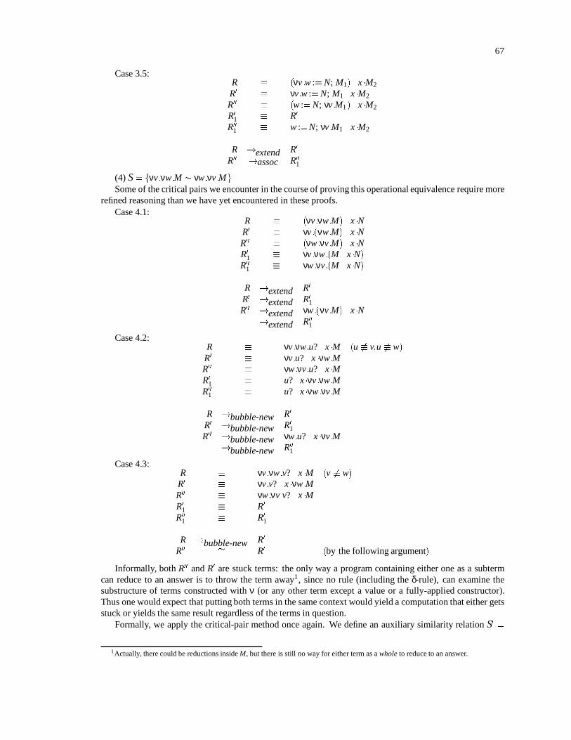
67

Case 3.5:R (νv:w := N; M1).x M2R0 νv:w := N; M1 .x M2R00 (w := N; νv:M1).x M2R01 R0

R001 w :=N; νv:M1 .x M2

R !extend R0

R00 !assoc R001

(4) S = fνv:νw:M νw:νv:MgSome of the critical pairs we encounter in the course of proving this operational equivalence require more

refined reasoning than we have yet encountered in these proofs.Case 4.1:

R (νv:νw:M).x NR0 νv:(νw:M) .x NR00 (νw:νv:M).x NR01 νv:νw:(M. x N)R001 νw:νv:(M. x N)

R !extend R0

R0 !extend R01R00 !extend νw:(νv:M) .x N

!extend R001

Case 4.2:R νv:νw:u? .x M (u 6 v;u 6 w)

R0 νv:u? .x νw:MR00 νw:νv:u? .x MR01 u?.x νv:νw:MR001 u?.x νw:νv:M

R !bubble-new R0

R0 !bubble-new R01R00 !bubble-new νw:u? .x νv:M

!bubble-new R001

Case 4.3:R νv:νw:v? .x M (v 6 w)

R0 νv:v? .x νw:MR00 νw:νv:v? .x MR01 R0

R001 R01

R !bubble-new R0

R00 = R0 (by the following argument)

Informally, both R00 and R0 are stuck terms: the only way a program containing either one as a subtermcan reduce to an answer is to throw the term away1, since no rule (including the δ-rule), can examine thesubstructure of terms constructed with ν (or any other term except a value or a fully-applied constructor).Thus one would expect that putting both terms in the same context would yield a computation that either getsstuck or yields the same result regardless of the terms in question.

Formally, we apply the critical-pair method once again. We define an auxiliary similarity relation S0 =

1Actually, there could be reductions inside M, but there is still no way for either term as a whole to reduce to an answer.

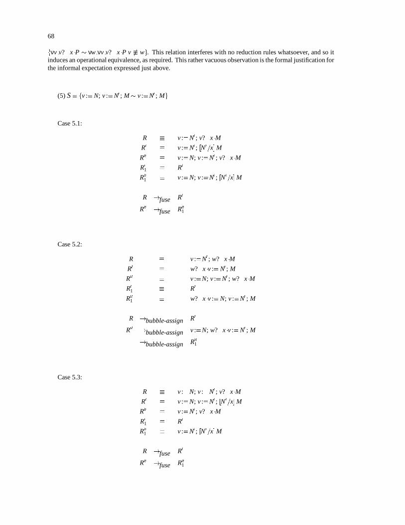
68

fνv:v? .x P νw:νv:v? .x Pjv 6 wg. This relation interferes with no reduction rules whatsoever, and so itinduces an operational equivalence, as required. This rather vacuous observation is the formal justification forthe informal expectation expressed just above.

(5) S = fv := N; v :=N0 ; M v :=N0 ; Mg

Case 5.1:

R v :=N0 ; v? .x M

R0 v :=N0 ; [N0=x]M

R00 v :=N; v :=N0 ; v? .x M

R01 R0

R001 v :=N; v :=N0 ; [N0=x] M

R !fuse R0

R00 !fuse R001

Case 5.2:

R v :=N0 ; w?.x M

R0 w?.x v := N0 ; M

R00 v :=N; v :=N0 ; w?.x M

R01 R0

R001 w?.x v := N; v :=N0 ; M

R !bubble-assign R0

R00 !bubble-assign v :=N; w?.x v := N0 ; M

!bubble-assign R001

Case 5.3:

R v :=N; v :=N0 ; v? .x M

R0 v :=N; v :=N0 ; [N0=x] M

R00 v :=N0 ; v? .x M

R01 R0

R001 v :=N0 ; [N0=x]M

R !fuse R0

R00 !fuse R001

69

Case 5.4:R v :=N; v :=N0 ; u?.x M (u 6 v)R0 v :=N; u?.x v := N0 ; MR00 v :=N0 ; u?.x MR01 u?.x v := N; v :=N0 ; MR001 u?.x v := N0 ; M

R !bubble-assign R0

R0 !bubble-assign R01R00 !bubble-assign R001

(6) For this equivalence, we adopt the similarity relation defined by S = fP .x " x Pg, where the meta-variable P ranges over procedures only. This similarity relation only interferes with the rule (assoc).

R (P .x " x).y Q

R0 P.x (" x.y Q)

R00 P.y Q

R01 P.x [x=y]Q

R001 R01

R !assoc R0

R0 !unit R01R00 R001

The last equivalence mentioned is just the α-renaming of R01.This concludes the proof of Proposition 4.2.1.

Proof: (7) S = fSeag [P] P j Seag[] an eager store-context, fv Seag[P] = fv P, and no free store-variable of Pis assigned in Seag[]gThis similarity relation can interfere both with the purification rules and with the assignment rules. All thecritical pairs having to do with the purification laws yield essentially the same diagram verification task, sowe give only a single example:

R pure(Seag [" (λx:M)])

R0 λx:pure Seag["M]

R00 pure(" (λx:M))

R01 R0

R001 λx:pure("M)

R !pure-eager R0

R00 !pure-eager R001

The uses of in the converse direction are equally simple to verify.The verification of the proof conditions in the cases of interference with assignment rules requires that we

invoke our knowledge concerning the structure of Seag[]. By the definition of a store-context (Figure 2.11),all assignments in Seag[] must be to tags defined in Seag[]. Also, we have assumed that Seag[] is nonempty, sothe immediate context of the metavariable M in the definition of S is either of the form νv:Seag [] or the formv :=N; Seag[]. We work out one of the three simple cases of interference with an assignment rule:

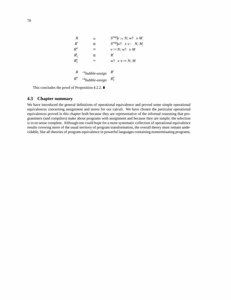
70

R Seag[v := N; w?.x M ]

R0 Seag[w? .x v := N; M]

R00 v :=N; w?.x M

R01 R0

R001 w?.x v := N; M

R !bubble-assign R0

R00 !bubble-assign R001

This concludes the proof of Proposition 4.2.2.

4.3 Chapter summaryWe have introduced the general definitions of operational equivalence and proved some simple operationalequivalences concerning assignment and stores for our calculi. We have chosen the particular operationalequivalences proved in this chapter both because they are representative of the informal reasoning that pro-grammers (and compilers) make about programs with assignment and because they are simple; the selectionis in no sense complete. Although one could hope for a more systematic collection of operational equivalenceresults covering more of the usual territory of program transformation, the overall theory must remain unde-cidable, like all theories of program equivalence in powerful languages containing nonterminating programs.

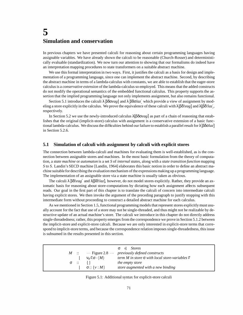
5Simulation and conservation

In previous chapters we have presented calculi for reasoning about certain programming languages havingassignable variables. We have already shown the calculi to be reasonable (Church-Rosser) and deterministi-cally evaluable (standardization). We now turn our attention to showing that our formalisms do indeed havean interpretation mapping procedures to state transformers on a suitable abstract machine.

We use this formal interpretation in two ways. First, it justifies the calculi as a basis for design and imple-mentation of a programming language, since one can implement the abstract machine. Second, by describingthe abstract machine in terms of a lambda-calculus with constants, we are able to establish that the eager-storecalculus is a conservative extension of the lambda-calculus so employed. This means that the added constructsdo not modify the operational semantics of the embedded functional calculus. This property supports the as-sertion that the implied programming language not only implements assignment, but also remains functional.

Section 5.1 introduces the calculi λ[βδσeag] and λ[βδσlaz] which provide a view of assignment by mod-eling a store explicitly in the calculus. We prove the equivalence of these calculi with λ[βδ!eag] and λ[βδ!laz],respectively.

In Section 5.2 we use the newly-introduced calculus λ[βδσeag] as part of a chain of reasoning that estab-lishes that the original (implicit-store) calculus with assignment is a conservative extension of a basic func-tional lambda-calculus. We discuss the difficulties behind our failure to establish a parallel result for λ[βδσlaz]in Section 5.2.6.

5.1 Simulation of calculi with assignment by calculi with explicit stores

The connection between lambda-calculi and machines for evaluating them is well-established, as is the con-nection between assignable stores and machines. In the most basic formulation from the theory of computa-tion, a state machine or automaton is a set S of internal states, along with a state transition function mappingS to S. Landin’s SECD machine [Landin, 1964] elaborates this basic notion in order to define an abstract ma-chine suitable for describing the evaluation mechanism of the expressions making up a programming language.The implementation of an assignable store via a state machine is usually taken as obvious.

The calculi λ[βδ!eag] and λ[βδ!laz], however, do not model stores explicitly. Rather, they provide an ax-iomatic basis for reasoning about store-computations by dictating how each assignment affects subsequentreads. Our goal in the first part of this chapter is to translate the calculi of concern into intermediate calculihaving explicit stores. We then invoke the argument of the preceding paragraph to justify stopping with thisintermediate form without proceeding to construct a detailed abstract machine for each calculus.

As we mentioned in Section 1.5, functional programming models that represent stores explicitly must usu-ally account for the fact that use of a store may not be single-threaded, and thus might not be realizable by de-structive update of an actual machine’s store. The calculi we introduce in this chapter do not directly addresssingle-threadedness; rather, this property emerges from the correspondence we prove in Section 5.1.2 betweenthe implicit-store and explicit-store calculi. Because we are only interested in explicit-store terms that corre-spond to implicit-store terms, and because the correspondence relation imposes single-threadedness, this issueis subsumed in the results presented in this section.

σ 2 StoresM ::= Figure 2.8 previously defined constructs

j νσ~v:σ hMi term M in store σ with local store-variables~vσ ::= fg the empty store

j σfv : Mg store augmented with a new binding

Figure 5.1: Additional syntax for explicit-store calculi

71

72

domσ The set of store-variables in the domain of σσ# v The binding of store-variable v in store σ, if one exists

σ! v : M The store having binding M for v, and all other bindings as in σ

Figure 5.2: Notation for explicit stores

νσ~v:σ hνv:Ni ! νσf~v;vg:σ hNi (σν)νσ~v:σ hv :=M; Ni ! νσ~v:(σ ! v : M : ) hNi (σ:=)

νσ~v:σ hv?.x Ni ! νσ~v:σ h[σ# v=x]Ni (v 2 domσ) (σ?)pureM ! νσfg:fg hMi (σblock )

f~v;vg ~v[fvg (abbreviation)

Figure 5.3: Common reduction rules for explicit-store calculi

νσ~v:σ h"(cn M1 Mk)i ! cn (νσ~v:σ h"M1i) (νσ~v:σ h"Mki) σpeag

νσ~v:σ h" f i ! f σpeag

νσ~v:σ h"λx:Mi ! λx:νσ~v:σ hMi σpeag

Figure 5.4: Reduction rules for eager explicit-store calculus λ[βδσeag]

νσ~v:σ hSlaz[" (cn M1 Mk)]i ! cn (νσ~v:σ hSlaz["M1]i) (νσ~v:σ hSlaz["Mk]i) σplaz

νσ~v:σ hSlaz[" f ]i ! f σplaz

νσ~v:σ hSlaz[" λx:M]i ! λx:νσ~v:σ hSlaz[M]i σplaz

Figure 5.5: Reduction rules for lazy explicit-store calculus λ[βδσlaz]

5.1.1 The calculi with explicit stores

The calculi λ[βδσeag] and λ[βδσlaz] are defined in Figures 5.1, 5.3, 5.4, and 5.5. The basic idea of these calculiis to replace rules fuse, bubble-assign, and bubble-new of λ[βδ!eag] and λ[βδ!laz] by rules for the explicitmanipulationof a store σ. Instead of acting as a boundary for observations, the pure construct initializes a storecomputation with an empty store. Instead of observations of the store bubbling from right to left, allocationof locations, updates, and reads are performed from left to right. The computation within a pure can thus beregarded as a machine execution embedded within the reductions of an expression-oriented calculus. Storesare unordered sets of bindings in which no store-variable is bound more than once; this is the same notion asthat of finite functions or records.

It is notable that the syntax for stores in Figure 5.1 admits arbitrary expressions for the value bound to astore-variable. This definition conforms to the semantics implied in the definitions of the implicit-store calculiλ[βδ!eag] and λ[βδ!laz]: the value stored is subject to the evaluation order of application, which is always by-name for our calculi. The distinctionbetween λ[βδ!eag] and λ[βδ!laz] lies in the evaluation order that pertainsto the relationship between a store-variable and the expression stored, which is an entirely orthogonal issue. Itwould be quite surprising if merely assigning an expression to a store-variable forced it to be reduced to weakhead normal form!

Figure 5.2 gives the meta-notations that we use in referring to explicit stores in this chapter. Like the no-tation [M=x]N that we use for substitution, these notations are not themselves part of the formal syntax of thecalculi, whereas the notation σ v : M is part of the formal syntax.

As Figure 5.1 shows, the explicit-store calculi extend λ[βδ!eag] and λ[βδ!laz] with an extra kind of termdenoting a term in the context of an explicit store. This syntactic construct is rather complex because thescoping of store-variable names is independent of the locality of stores in our calculi. The term νσ~v:σ hMideclares a set of store-variables ~v fv1 ;: : : ;vng;n 0 to be local to the notated store σ and to the term M

73

(we use ~v as a compact notation for such a set of variables). The store σ may contain bindings of non-localstore-variables, and the terms bound to store-variables may contain non-local store-variables.

The syntax νσ~v:σ hMi is intended to be used when M is a command; however, other terms are not prohib-ited (although we do not assign them an informal meaning—they will all become “stuck”). It is not possible toprohibitnested occurrences of νσ~v:σ hMibecause this syntax models pure-expressions, and pure-expressionscan be nested. We tolerate the proliferation of meaningless terms based on this syntax because we intend touse the explicit-store calculi primarily as a target of translation from λ[βδ!eag] and λ[βδ!laz]; the terms thatdo not actually occur as translations are thus filtered out naturally.

The reduction rules specified in Figure 5.3 make use of the notations for explicit stores that are tabulated inFigure 5.2. These rules are straightforward transcriptions of the meaning of the various assignment constructsinto the notation of explicit stores. Since our notation for explicit stores separates the declaration of the exis-tence of a store-variable from its binding in the store, an undefined store-variable is represented by its absencefrom the store in which it is sought—this is the side condition on rule σ?. Rule σν merely transfers the localscope of the newly-declared store-variable from the command sequence in which it occurs to the explicit storein which the command was encountered. As always in this dissertation, we observe Barendregt’s conventionthat bound and free names are distinct; there is thus no danger of semantic gibberish resulting from capture ofoccurrences of v in σ because the bound v is really α-renamed behind the reduction arrow where we can’t seeit. We also note that rule σ:= is indifferent to the prior existence of a binding for v in the store σ and that allof the rules are indifferent to the locality of declaration of a store-variable.

Rule σblock initializes a store; it corresponds to a pure boundary in λ[βδ!eag] and λ[βδ!laz].The eager- and lazy-store versions of the explicit-store calculus differ, as before, in the rules for propagat-

ing the store into the subterms of a returned value. In the eager version (Figure 5.4), all store actions must havebeen reduced away before the store is pushed past a constructor of the result; this corresponds to the structureof store contexts Seag[], in which there may be no outstanding reads. In the lazy version (Figure 5.5), the storemay be pushed past the constructor as soon as the fact that a result is returned can be seen from the structure ofthe argument to pure; this corresponds to the more lenient lazy store contexts Slaz[]. The presence of the store-context in the rules in Figure 5.5 reflects the possibility of pushing the store-computation into the structure ofa result term before having executed all the commands in the context.

The calculi λ[βδσeag] and λ[βδσlaz] have both the Church-Rosser property and standard orders of re-duction. Because the proof techniques involved are basically a repetition of the corresponding proofs forλ[βδ!eag] and λ[βδ!laz] in Chapter 3, we have placed the proofs of these properties for λ[βδσeag] and λ[βδσlaz]in Appendix A.

In the following discussion of explicit-store calculi reductions in an explicit-store calculus are denoted!σ where the distinction is not obvious from the context. Figure 5.2 gives several other notatio used in thefollowing exposition.

5.1.2 Equivalence of bubble/fuse rules and store-transition rules

In Section 5.1.1, we introduced calculi that represent a store explicitly. In this section, we consider programsin λ[βδ!eag] and λ[βδ!laz] under the reduction rules of λ[βδσeag] and λ[βδσlaz]; since every term of eachimplicit-store calculus is also a legal term of the corresponding explicit-store calculus this endeavor makessense. We show that such programs are assigned the same semantics by both the explicit-store and the implicit-store calculi.

The central step in establishing this equivalence is to establish the correspondence of λ[βδ!eag]or λ[βδ!laz]terms with λ[βδσeag] or λ[βδσlaz] terms such that the correspondence relates terms in different calculi thathave the same informal meaning as store operations. We first define the correspondence relation and then show(in a sense to be defined) that the correspondence is preserved under reductions.

In the following definition, we refer to eager store-contexts Seag[] despite the fact that the definition isapplicable to lazy-store calculi as well: we are referring only to the syntactic form of such contexts, not totheir role in defining reductions for eager-store calculi.

The correspondence relation, which we denote by the symbol b=, relates terms of an implicit-store cal-culi and terms of explicit-store calculi. The relation links a term of λ[βδ!eag] or λ[βδ!laz] (on the left) andλ[βδσeag] and λ[βδσlaz] (on the right). We define b= by means of two mutually inductive sets of inference

74

MM0

M b=M0

Seag[] b= νσ~v:σ h[]i M b=M0

pureSeag[M] b= νσ~v:σ hM0i

M b=M0 N b=N0

MN b=M0 N0

M b=M0

λx:M b= λx:M0

M b=M0

νv:M b= νv:M0

M b=M0

M? b=M0?

M b=M0 N b=N0

(M := N) b= (M0 :=N0 )

M b=M0 N b=N0

(M. x N) b= (M0 .x N0 )

M b=M0

"M b= "M0

M b=M0

pureM b= pureM0

Figure 5.6: The correspondence relation for terms

[] b= νσfg:fg h[]i

Seag[] b= νσ~v:σ h[]iνSeag []:b=νσf~v;vg:σ h[]i

Seag[] b= νσ~v:σ h[]i M b=M0

(v 62 domσ)v :=M; Seag[] b=νσ~v:σ ! v : M0 h[]i

Seag[] b= νσ~v:σ h[]i(v 2 domσ)

v :=M; Seag[] b=νσ~v:σ h[]i

Figure 5.7: The correspondence relation for store-contexts and stores

rules given in Figure 5.6. The rule whose hypothesis is MM0 acts as the axiom for the inference system; allbut one of the other rules are those we would expect if we were defining b= to be a congruence. The exception isthe rule involving pure, which acts as the interface to the definition of correspondence between store-contexts(on the left) and explicit stores (on the right) given in Figure 5.7.

Among the inference rules given in Figure 5.7 there is an obvious axiom relating empty store-contexts andempty stores. The rule for store-variable declaration straightforwardly relates the declaration mechanisms inthe two pairs of calculi. The remaining rules implement the informal notion that the store corresponding to animplicit store-context records only the most recent (innermost) assignment to a store-variable; the presence ofan overriding binding is detected by the presence of the store-variable in the domain of the store given by anested application of the inference rules. The interface back into the rules for terms is the hypothesis M b=M0

of the rule for introducing the actually effective assignment into both contexts.This definition of correspondence implies that every term or store in an explicit-store calculus has a cor-

responding term or store context in an implicit-store calculus:

Lemma 5.1.1 (i) For any term M in an explicit-store calculus, there exists a term implicit(M) in the cor-responding implicit-store calculus such that implicit(M) b= M.

(ii) Likewise, for any explicit store context νσ~v:σh []i there exists an implicit store-context Seag[]= implicit(σ)such that Seag[] b= νσ~v:σ h[]i.

Proof: The proof consists of the obvious structural induction. The base cases for terms are the terminal syn-tactic classes; the induction for terms is by the rules in Figure 5.6, and that for contexts is by the rules inFigure 5.7.

The next lemma assures that reductions in the explicit-store calculi act as an inverse to implicit, in thatthey actually build, step by step, a store corresponding to a store context.

75

Lemma 5.1.2 For any term M and store context Seag[] in an explicit-store calculus there is an explicit storecontext νσ~v:σ h[]i such that Seag[] b= νσ~v:σ h[]i and such that

pureSeag[M]! νσ~v:σ hMi:

Proof: We can immediately apply a σblock -reduction to the initial term, giving pureSeag[M]!fg hSeag[M]i.A straightforward induction on the structure of Seag[], carrying out σ:=- and σν-reductions as required, buildsa store that corresponds to Seag[].

Now we come to the central lemma in our proof that explicit-store computations simulate implicit-storereductions.

Lemma 5.1.3 Given terms M0 and N0 in an explicit-store calculus, and term M b= M0 in the correspondingimplicit-store calculus, if M0!σ N0 , then there is a term N such that N b=N0 and M! N.

In a picture, there exists a term N that makes the following diagram commute:

M0

M N

N0

b=

-.........

b=

. . . . . . . . .--

Proof: We decompose the problem into one case for each possible reduction rule that might give M0! N0 .Since the relation b= distributes through all term-forming operators in the explicit-store calculus, we can as-sume without loss of generality that the redex in M0!N0 is the whole term M0.

If M0 is a β-, δ-, assoc-, extend-, unit-, or assign-result-redex, the result follows immediately, since theserules are also reduction rules in the corresponding implicit-store calculus: we just take M M0, N N0 .

The remaining cases are as follows. We use Lemma 5.1.1 freely without mention.

Case (1) M0 νσ~v:σ hνv:P0 i.

In this case, M pureSeag[νv:P] for some eager store context Seag[] and term P such that Seag[] b=νσ~v:σ h[]i and P b=P0 . The result of the lemma then follows from the diagram

νσ~v:σ hνv:P0 i

pureSeag[νv:P]:

νσf~v;vg:σ hP0 i-

b=

b=

Case (2) M0 νσ~v:σ hv :=M0

2; P0 i

In this case M pureSeag[v := M2; P] for some store context Seag[] and terms M2 and P such that

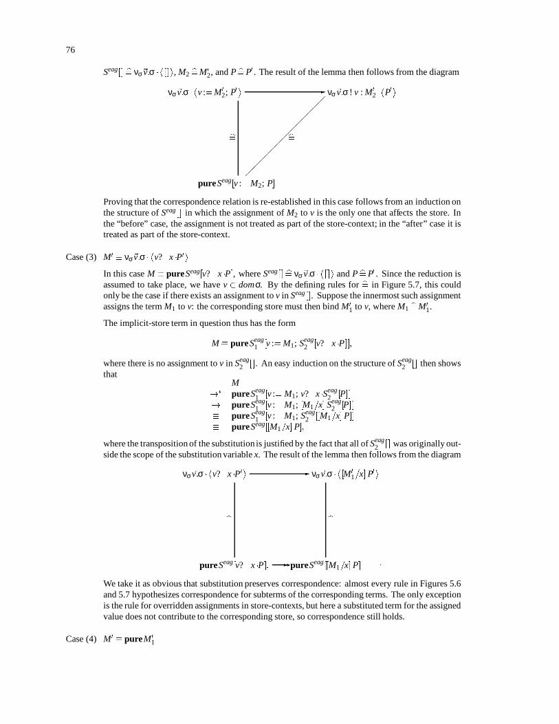
76

Seag[] b= νσ~v:σ h[]i, M2 b=M0

2, and P b=P0 . The result of the lemma then follows from the diagram

νσ~v:σ hv :=M0

2; P0 i

pureSeag[v := M2; P]:

νσ~v:σ ! v : M0

2 hP0 i-

b=

b=

Proving that the correspondence relation is re-established in this case follows from an induction onthe structure of Seag[] in which the assignment of M2 to v is the only one that affects the store. Inthe “before” case, the assignment is not treated as part of the store-context; in the “after” case it istreated as part of the store-context.

Case (3) M0 νσ~v:σ hv? .x P0 i

In this case M pureSeag[v? .x P], where Seag[] b= νσ~v:σ h[]i and P b=P0 . Since the reduction isassumed to take place, we have v 2 domσ. By the defining rules for b= in Figure 5.7, this couldonly be the case if there exists an assignment to v in Seag[]. Suppose the innermost such assignmentassigns the term M1 to v: the corresponding store must then bind M0

1 to v, where M1 b=M0

1.

The implicit-store term in question thus has the form

M pureSeag1 [v := M1; Seag

2 [v? .x P]];

where there is no assignment to v in Seag2 []. An easy induction on the structure of Seag

2 [] then showsthat

M! pureSeag

1 [v := M1; v?.x Seag2 [P]]

! pureSeag1 [v := M1; [M1=x] Seag

2 [P]] pureSeag

1 [v := M1; Seag2 [[M1=x]P]]

pureSeag[[M1=x]P];

where the transposition of the substitution is justified by the fact that all of Seag2 [] was originally out-

side the scope of the substitution variable x. The result of the lemma then follows from the diagram

νσ~v:σ hv? .x P0 i

pureSeag[v? .x P]:

νσ~v:σ h[M0

1=x]P0 i

pureSeag[[M1=x]P]--

-

b= b=

:

We take it as obvious that substitution preserves correspondence: almost every rule in Figures 5.6and 5.7 hypothesizes correspondence for subterms of the corresponding terms. The only exceptionis the rule for overridden assignments in store-contexts, but here a substituted term for the assignedvalue does not contribute to the corresponding store, so correspondence still holds.

Case (4) M0 pureM0

1

77

In this case M pureM1 for some M1 b=M0

1. The result of the lemma follows from the diagram

pureM0

1

pureM1:

νσfg:fg hM0

1i-

b=

b=

Case (5) (λ[βδσeag] only) M0 νσ~v:σ h"(λx:M0

1)i

We take this case as representative of the purification reductions; the proofs in the other cases aresimilar. In this case M pureSeag[" (λx:M1)], where Seag[] b=~v hσi[] and M1 b=M0

1. The result ofthe lemma then follows from the diagram

νσ~v:σ h" (λx:M0

1)i

pureSeag[" (λx:M1)]

λx:νσ~v:σ h"M0

1i

λx:pure Seag["M1]:

-

-

b= b=

Case (6) (λ[βδσlaz] only) M0 νσ~v:σ hSlaz[" (λx:M0

1)]i

Again, we take this case as representative of the purification reductions. The proofs in the othercases are similar. In this case M pureSeag[Slaz

1 [" (λx:M1)]], where Seag[] b= νσ~v:σ h[]i, and

Slaz1 [" (λx:M1)] b= Slaz

1 [" (λx:M0

1)]:

Noting that every eager store-context is also a lazy store-context, and that the nesting of two lazystor- contexts is again a lazy store context, we have the diagram

νσ~v:σ hSlaz[" (λx:M0

1)]i

pureSeag[Slaz1 [" (λx:M1)]]

λx:(νσ~v:σ hSlaz["M0

1]i)

λx:(pure Seag[Slaz1 ["M1]]):

-

-

b= b=

:


The maintenance of correspondence under reduction established by Lemma 5.1.3 forms the core of themain simulation theorem (Theorem 5.1.7), but the full theorem requires some additional lemmas concerningthe action of imperative reductions in the implicit-store calculi on the form of store contexts. We now begin a

78

series of results intended to characterize the behavior of reductions in command sequences in λ[βδ!eag] andλ[βδ!laz].

Our first lemma notes that much of the structure of command sequences is preserved “up to bubbling” byreductions in the implicit-store calculi.

Definition 5.1.4 A bubble context is a context defined by the productions

B[] ::= [] j v?.x B[ ]:

Lemma 5.1.5 (Persistence of store-context) Assume that λ[βδ!eag] ` M! M0 or λ[βδ!laz] ` M! M0.Then:

(i) If M νv:N then there is a term N0 and a bubble context B[] such that M0 B[νv:N0 ].

(ii) If M v :=N; P then there are terms N0 and P0 and a bubble context B[] such that M0 B[v := N0 ; P0 ].

(iii) If M "N then there is a term N0 such that M0 "N0 .

(iv) If M v?.x P then there is a term P0 such that M0 v? .x P0 .

Proof: By inspection of the reduction rules for λ[βδ!eag] and λ[βδ!laz], it is clear that only the rules pure-eagerand pure-lazy can remove a ν or := from a term. Furthermore, there is no rule that can reduce a term prefixedwith one of these constructs to one that has it only within the context of a pure. The only remaining reductionrules that explicitly involve terms of the form in (i) and (ii) are the rules bubble-assign and bubble-new, whichclearly act to embed the former top-level constructs within a bubble context. Similar reasoning establishes (iii)and (iv).

The next result shows that, if reduction of a command-redex is essential in a computation that produces ananswer, then that redex must occur in the context of a pure-expression. The informal notion of “essential” isrepresented by being a head redex. The proof of Lemma 5.1.6 argues in several places that a stuck reductionin an evaluation context prevents a term from reducing to an answer. In this form of reasoning, getting stuckmeans never reducing either to part of an answer or to a subterm that makes some containing term a redex.This clearly prevents the standard reduction from progressing to an answer, and hence the whole term couldnot have reduced to an answer in the first place.

Lemma 5.1.6 (Only pure purifies) Let M be a term in λ[βδ!eag] or λ[βδ!laz], and assume that ME[∆h ]!

A, where ∆h is a fuse-, bubble-assign-, or bubble-new-redex that is head redex in M.Then there is an evaluation context E1[] and an eager store context Seag[] such that M E1[pure Seag[∆h ]].

Proof: Assume the contrary, that is, that M is not of the required form. We consider each remaining possiblestructure of the term M (as determined by the structure of the evaluation context E[]) and show, as a contra-diction, that these structures cannot reduce to an answer.

Case (1) If E[] Seag[] for some store-context Seag[], then Lemma 5.1.5 applies to show that M 6! A, andwe have an immediate contradiction.

Case (2) The alternative is that the structure of E[] is interrupted by some nested evaluation context that isnot also an eager store-context. We introduce names for the contexts implied by this statment byasserting that E[] E1[E2 [Seag []]], where E1[] is an evaluation context, E2[] is a non-empty evalu-ation context that is not an unrestricted store context, and Seag[] is an eager store-context. Withoutloss of generality, we can assume that E1[] [] and that E2[] is minimal, that is, that E2[] can beobtained by exactly one application of a production in Figures 3.2, 3.3, and 3.4. We subdivide thiscase according to the form of E2[].

79

Case (2a) E2[] [] N.Assume Seag[∆h ]!

A. By Theorem 3.7.10, we can choose the reduction sequenceto reduce ∆h first. By Lemma 5.1.5, the reduction can only yield a term of the formB[Seag

1 [N1 ]], where N1 cannot be an abstraction. Such a residual term can only inter-act with its context Seag[] by means of one of the rules bubble-assign or bubble-new;hence, there is no way to reduce Seag[∆h ] to an abstraction or to a primitive-functionname. There can thus be no way to reduce the application to an answer; this is the de-sired contradiction.

Case (2b) E2[] f [].The argument for this case is similar to that for Case (2a), noting instead that Seag[∆h ]can reduce neither to an abstraction nor to a constructed value.

Case (2c) E2[] []?, E2[] [] :=N, E2[] pureSeag[" []].These cases are all similar to Case (2a).

Case (2d) E2[] [] .x N.In this case E2[Seag [∆h ]] is a redex, contradicting the assumption that ∆h is the head redex(outermost evaluation redex).

Case (2e) E2[] N1 .x [ ].For this case to apply, N1 cannot have the form E3[∆] for any evaluation context E3[] andredex ∆, because this would make ∆, not ∆h, the head redex; in other words, N1 must bein head normal form. Also, N1 .x ∆h itself cannot be a redex for the same reason. ThusN1 cannot have any of the forms N2 .y N3 , "N2 , or νv:N2 . Furthermore, if N1 has theform N2 :=N3 then N2 is not a store-variable, because then E2[] would be an eager store-context, which it was assumed not to be. Now by Lemma 5.1.5, ∆h!

B[Seag [N0

1 ]], soa head-reduction sequence will bubble the store-variable-reads that are outermost in B[]to the left, where they cannot interact with any of the remaining possible forms for N1 .Hence the entire term cannot reduce to an answer.

Case (2f) E2[] νv:[ ], E2[] v :=N .x [ ], E2[] " [].These cases all contradict the assumption that E2[] is not an eager store context.

Case (2g) (in λ[βδ!eag]) E2[] pureSeag1 [" ].

In this case M pureSeag1 [Seag [" ∆h]].

By Lemma 5.1.5 or by inspection of the set of reduction rules the residuals of ∆h aresyntactically all command-sequences, having . as their top-level syntactic constructor.There is thus no way for these residuals to interact with their containing" construct, andhence it is impossible for M to reduce to an answer, a contradiction.

Case (2h) (in λ[βδ!laz]) E2[] pureSlaz1 [].

In this case M pureSlaz1 [Seag [∆h ]], and we proceed by the same reasoning as that used

for the corresponding case in λ[βδ!eag].

The only remaining case is E2[] pure[], hence we must have

M E1[E2 [Seag [∆h ]]] E1[pure Seag[∆h ]]:

But this proves Lemma 5.1.6.

We are now prepared to state and prove the main theorem on the mutual simulation between λ[βδ!eag]and λ[βδ!laz] on the one hand and λ[βδσeag] and λ[βδσlaz] on the other. The notion of operational seman-tics we use in this proof is of reduction to a constant c0. It is possible to extend this semantics to compoundanswers at the meta-level by testing several programs, each of which is the application of a composition ofselection primitives to the original program. We restrict the form of answer considered because standard re-duction sequences to constants have a particularly simple form: they are always head reduction sequences (byTheorem 3.7.12).

80

Theorem 5.1.7 For every closed term M and constant c0,

(i) λ[βδ!eag] `M = c0 if and only if λ[βδσeag] `M = c0.

(ii) λ[βδ!laz] `M = c0 if and only if λ[βδσlaz] `M = c0.

Proof: We first prove the “only if” direction of the implications.Assume that λ[βδ!eag] `M = c0. By Theorem 3.7.12 there exists a head reduction sequence reducing M

to c0. We now carry out an induction on the length of this head reduction sequence.The base case of the induction is a reduction sequence of length zero, in which case M c0 and there is

nothing to show.For the induction step, assume that the statement of the theorem holds for head reduction sequences of

length n or less, and consider M such that M! c0 by head reductions in n+ 1 steps (in the implicit-storecalculus). Then the head reduction sequence from M has the form

M E[∆]! E[L] M0! c0

for some evaluation context E[], head redex ∆, and terms L and M0. We now show that λ[βδσeag] `M = M0

by a case analysis on the form of ∆.

Case 1: If ∆ is a β-, δ-, assoc-, extend-, assign-result-, or unit-redex, the result is immediate because thesereduction rules apply in λ[βδσeag] and λ[βδσlaz] as well.

Case 2: ∆ v :=N; v?.x P

By Lemma 5.1.6 there is an evaluation context E[] and an eager store context Seag[] such that

M E[pure Seag[v := N; v? .x P]]:

By Lemma 5.1.2, M! Mσ in the explicit-store calculus, where

Mσ E[νσ~v:σSeag [] hv :=N; v?.x Pi];

where νσ~v:σSeag [] h[]i is the explicit store context whose existence is guaranteed by Lemma 5.1.1.

Then we have the followingderivation that λ[βδσeag]`Mσ = M0, which in turn implies λ[βδσeag]`M = c0 via the transitivity of conversion.

Mσ E[νσ~v:σSeag [] hv :=N; v?.x Pi]! E[νσ~v:σSeag [] ! v : N hv? .x Pi] (σ:=)! E[νσ~v:σSeag [] ! v : N h[N=x]Pi] (σ?) E[pure Seag[v := N; [N=x]P]] (Lemma 5.1.2, σ:=) M0

This derivation works equally well for λ[βδ!laz] being simulated by λ[βδσlaz].

Case 3: ∆ v :=N; w?.x P

Reasoning as in the previous case, we have

M E[pure Seag[v := N; w?.x P]]!Mσ;

whereMσ E[νσ~v:σSeag [] hv :=N; w?.x Pi]:

We now have the following derivation showing that λ[βδσeag] ` Mσ = M0. We are assured thatSeag[] contains an assignment to w because we know that the store-context eventually reduces away;whereas a read of an unassigned variable w bubbles leftward to meet either the pure or a declaration

81

of w. It must do so via head reductions because we know that the spine of a store-context with apure within an evaluation context is itself within an evaluation context.

Mσ E[νσ~v:σSeag [] hv :=N; w?.x Pi]! E[νσ~v:σSeag [] ! v : N hw?.x Pi] (σ:=)! E[νσ~v:σSeag [] ! v : N h[σ0 #w=x]Pi] (σ?) E[νσ~v:σSeag [] hv :=N; [σ0 #w=x]Pi] (σ:=) E[νσ~v:σSeag [] h[σ0 #w=x] (v := N; P)i] (Note: x 62 fv N) E[νσ~v:σSeag [] hw?.x v := N; Pi] (σ?) E[pure Seag[w? .x v := N; P]] (Lemma 5.1.2) M0

Case 4: ∆ νv:w? .x P;v 6= w

Once again we invoke Lemma 5.1.6 to place our redex ∆ in context as

M E[pure Seag[νv:w? .x P]]:

Lemma 5.1.2 allows us to begin the following derivation of the desired result. Our assurance that wis bound in the store rests here on the same ground as in the previous case.

M ! E[νσ~v:σSeag [] hνv:w? .x Pi] (Lemma 5.1.2)! E[νσf~v;vg:σSeag [] hw?.x Pi] (σν)! E[νσf~v;vg:σSeag [] h[σSeag [] #w=x]Pi] (σ?) E[νσ~v:σSeag [] hνv:[σSeag [] #w=x]Pi] (σν) E[νσ~v:σSeag [] h[σSeag [] #w=x] νv:Pi] E[νσ~v:σSeag [] hw?.x νv:Pi] (σ?) E[pure Seag[w? .x νv:P]] Lemma 5.1.2 M0:

Case 5: (λ[βδ!eag]/λ[βδσeag] only) ∆ pureSeag[" (λx:M)].

Again using Lemma 5.1.2, we have:

M E[pure Seag[" (λx:M)]]! E[νσ~v:σSeag [] h"(λx:M)i] (Lemma 5.1.2)! E[λx:νσ~v:σSeag [] h"Mi] (σblock ) E[λx:pure Seag["M]] (Lemma 5.1.2) M0:

The cases of the other pure-eager-reduction rules behave similarly.

Case 6: (λ[βδ!laz]/λ[βδσlaz]/ only) ∆ pureSlaz[" (λx:M)].

By the same general form of reasoning as in the other cases, we have

M E[pure Slaz[" (λx:M)]]! E[νσfg:fg hSlaz[" (λx:M)]i] (σblock)

E[λx:νσfg:fg hSlaz["M]i] (σplaz ) E[λx:pure Slaz["M]] (σblock) M0:

This concludes the proof that λ[βδ!eag] `M = c0 implies λ[βδσeag] `M = c0.

82

We establish the converse by applying Lemma 5.1.3. Assume that λ[βδ!eag 0] `M = c0. By the definitionof (b=), M b=M; furthermore, c0 b=c00 implies c0 c00. The theorem can then be established by pasting togetherdiagrams of the form provided by Lemma 5.1.3 as follows:

M M0

1 c0

M M1 c0

-σ

-σ

- -

b= b= b=

. . . . . . . .

. . . . . . . .

This concludes the proof of Theorem 5.1.7.

5.2 Calculi with assignments as conservative extensions of lambda-calculi

Every term and reduction in the calculus λ[βδ] is also a term or reduction of λ[βδ!eag] and λ[βδ!laz]. Henceany convertibility relation that holds in λ[βδ] must also hold in λ[βδ!eag] and λ[βδ!laz]. We recall from Chap-ter 4, however, that the operational-equivalence theory of a lambda-calculus is really the interesting theory forreasoning about programs. The definition of operational equivalence involves a universal quantification overall contexts in a calculus. When we embed a term from λ[βδ] into a calculus with assignments, some of thesecontexts will contain constructs that are not present in the original λ[βδ]. We could thus conceive of a situ-ation in which the operational-equivalence theory of the imperative calculus either equates or distinguishesλ[βδ]-terms that are not equated or distinguished by the operational-equivalence theory of λ[βδ].

In this section, we show that the calculi λ[βδ!eag] is, in fact, a conservative extension of λ[βδ]: it preservesthe operational-equivalence theory of λ[βδ] exactly. The strategy we employ is to give meaning-preservingtranslations in both directions between the language of λ[βδσeag] and the language of λ[βδ] with specially-designed primitives that carry out a simulation of the imperative constructs. The preservation of meaning,along with the definability of the constructs in λ[βδ], is sufficient to establish conservative extension.

Before we prove this result we must be more precise about what we actually prove. Because we have leftthe constructors and primitive functions unspecified, every one of the “calculi” proposed in this dissertationis actually an entire family of calculi. Up to this point, we have not belabored this distinction because allour results have held uniformly for all calculi in each family. We must now break this pattern in order to beprecise about our conservative-extension results, since it is not the case that every calculus with assignment isan extension of every member of the family λ[βδ]. Instead, for each calculus with assignment we will showthat there exists a member of the family λ[βδ] for which the original calculus is a conservative extension. Theproof of conservative extension will use this freedom to construct a basic lambda-calculus in an essential way:the constructs implementing the translation from the calculi with assignments will be new primitives withina basic lambda-calculus, and we will construct inverse translations that recognize these primitives as such.

We actually carry out the proof of conservative extension using the explicit-store calculus λ[βδσeag]; wethen use the results of Section 5.1 to conclude that λ[βδ!eag] itself is a conservative extensions of λ[βδ] in thesense in which we use the term here. The proof that λ[βδσeag] is a conservative extension of λ[βδ] is itselfmediated by a translation into a calculus λν devised by Odersky [Odersky, 1993b; Odersky, 1994]; Oderskyhas shown λν to be a conservative extension of λ[βδ]. Section 5.2.1 introduces the technical notion of syn-tactic embedding which forms the backbone of the proof. Section 5.2.2 introduces the relevant features ofthe calculus λν, Section 5.2.3 details the translation from λ[βδσeag] into λν, Section 5.2.4 gives an inversetranslation that is needed to show the existence of a syntactic embedding, and Section 5.2.5 joins the piecestogether to give a proof of conservative extension. Section 5.2.5 comments on the difficulty of carrying outthis process for λ[βδσlaz].

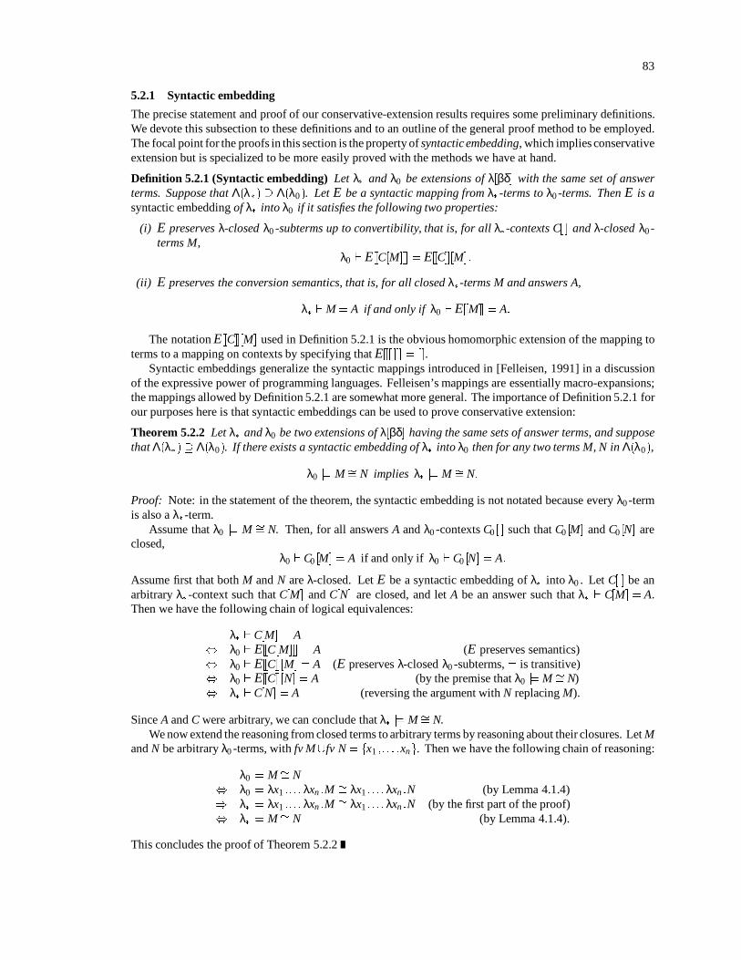
83

5.2.1 Syntactic embedding

The precise statement and proof of our conservative-extension results requires some preliminary definitions.We devote this subsection to these definitions and to an outline of the general proof method to be employed.The focal point for the proofs in this section is the property of syntactic embedding, which implies conservativeextension but is specialized to be more easily proved with the methods we have at hand.

Definition 5.2.1 (Syntactic embedding) Let λ and λ0 be extensions of λ[βδ] with the same set of answerterms. Suppose that Λ(λ ) Λ(λ0 ). Let E be a syntactic mapping from λ -terms to λ0 -terms. Then E is asyntactic embedding of λ into λ0 if it satisfies the following two properties:

(i) E preserves λ-closed λ0 -subterms up to convertibility, that is, for all λ -contexts C[ ] and λ-closed λ0 -terms M,

λ0 ` E[[C[M]]] = E[[C]][M]:

(ii) E preserves the conversion semantics, that is, for all closed λ -terms M and answers A,

λ `M = A if and only if λ0 ` E[[M]] = A:

The notation E[[C]][M] used in Definition 5.2.1 is the obvious homomorphic extension of the mapping toterms to a mapping on contexts by specifying that E[[[ ]]] = [].

Syntactic embeddings generalize the syntactic mappings introduced in [Felleisen, 1991] in a discussionof the expressive power of programming languages. Felleisen’s mappings are essentially macro-expansions;the mappings allowed by Definition 5.2.1 are somewhat more general. The importance of Definition 5.2.1 forour purposes here is that syntactic embeddings can be used to prove conservative extension:

Theorem 5.2.2 Let λ and λ0 be two extensions of λ[βδ] having the same sets of answer terms, and supposethat Λ(λ ) Λ(λ0). If there exists a syntactic embedding of λ into λ0 then for any two terms M, N in Λ(λ0),

λ0 j= M= N implies λ j= M = N:

Proof: Note: in the statement of the theorem, the syntactic embedding is not notated because every λ0 -termis also a λ -term.

Assume that λ0 j= M = N. Then, for all answers A and λ0 -contexts C0 [ ] such that C0 [M] and C0 [N] areclosed,

λ0 ` C0 [M] = A if and only if λ0 ` C0 [N] = A:

Assume first that both M and N are λ-closed. Let E be a syntactic embedding of λ into λ0 . Let C[ ] be anarbitrary λ -context such that C[M] and C[N] are closed, and let A be an answer such that λ ` C[M] = A.Then we have the following chain of logical equivalences:

λ ` C[M] = A, λ0 ` E[[C[M]]] = A (E preserves semantics), λ0 ` E[[C]][M] = A (E preserves λ-closed λ0 -subterms, = is transitive), λ0 ` E[[C]][N] = A (by the premise that λ0 j= M = N), λ ` C[N] = A (reversing the argument with N replacing M).

Since A and C were arbitrary, we can conclude that λ j= M= N.We now extend the reasoning from closed terms to arbitrary terms by reasoning about their closures. Let M

and N be arbitrary λ0 -terms, with fv M[fv N = fx1 ;: : : ;xng. Then we have the following chain of reasoning:

λ0 j= M= N, λ0 j= λx1 :: : : λxn :M = λx1 :: : : λxn :N (by Lemma 4.1.4)) λ j= λx1 :: : : λxn :M = λx1 :: : : λxn :N (by the first part of the proof), λ j= M= N (by Lemma 4.1.4).

This concludes the proof of Theorem 5.2.2

84

v 2 Local names

M ::= (Figure 2.2) j νv:M local name v over scope Mj M1 == M2 test of name equality

Figure 5.8: Syntax of the local-name calculus λν

(Figure 2.3) νn:cm M1 Mk ! cm (νn:M1) (νn:Mk ): λνcn

νn:λx:M ! λx:νn:M: λνλv== v ! true λν ==v== w ! false (v 6 w) λν ==

Figure 5.9: Reduction rules for the local-name calculus λν

5.2.2 The calculus λν

Before we prove the conservative-extension theorem for the calculi of concern, we quickly state why findinga syntactic embedding of those calculi into λ[βδ] is nontrivial. A natural implementation of a store calculus interms of λ[βδ] maps assignments and reads to read and write operations on an actual store. This suggests usingthe explicit-store calculi defined earlier in this chapter as an intermediate step in the implementation. Becauseall operational equivalences of λ[βδ!eag] and λ[βδ!laz] are preserved in the corresponding explicit-store cal-culi, proving our conservative-extension results for the explicit-store calculi will immediately establish theresults for the implicit-store calculi as well.

With this scheme in mind, a store from an explicit-store calculus can be represented in λ[βδ] as a mappingfrom store-variables to terms. Unfortunately, store-variables have no obvious corresponding entity in λ[βδ]:they are pure names with scope and a test for equality, but they are not locuses of substitutionas are the normalλ-variables. We can try to encode the allocation of names by some technique from pure functional program-ming, such as passing around a supply of names, but then we cannot fulfill the part of the definition of syntacticembedding that demands that closed programs in the target calculus as found in the extended calculus map tothemselves—name-supply passing is a pervasive transformation (as is continuation-passing).

The papers [Odersky, 1993b; Odersky, 1994] define a calculus λν which specifically solves this problem.Rather than attempting any implementation of locations as some more primitive entity, Odersky’s calculusprovides a direct axiomatization of the important properties of distinct names defined over scopes. The calcu-lus λν is itself a conservative extension of λ[βδ], so it provides another suitable intermediate calculus for theoverall proof that the calculi of concern conservatively extend λ[βδ]. Odersky’s proof that λν forms a con-servative extension of λ[βδ] constructs a syntactic embedding from λν to λ[βδ] that encodes a de Bruijn-likelevel-numbering scheme for the name bindings into the target lambda calculus. The technique of translatingλν-terms into a name-supply-passing style is ruled out by the requirement that a syntactic embedding mustpreserve those λ[βδ]-terms that are present in λν.

Basically, λν adds only one feature to λ[βδ]: the name-introductionconstruct νn:M, along with a primitive== for detecting the equality of names. To the reader of this dissertation, therefore, λν may just seem like astripped-downversion of our calculi with assignment. The reduction rules of λν are all the rules of λ[βδ] (givenin Figure 2.3) augmented as given in Figure 5.9. The calculus λν does not require any construct analogous topure to demarcate subterms over which local names are in use—the entire term acts as the unit of ‘purification’when we are concerned to get rid of local names.

Rule λνcn allows the scope of a local name to be pushed down through a constructed value; the splittingofthe scope is rationalized in much the same fashion as the splitting of the store-context in the purification rulesof λ[βδ!eag] and λ[βδ!laz]. Rule λνλ allows the scope of a local name to be pushed down through a lambda-abstraction. This allows the lambda-abstraction to be exposed, perhaps to participate in a β-reduction thatplaces the argument of the lambda inside of the name’s scope: this is a characteristic mode of computation in

85

λν. As usual, the bound names v are α-renamable, and we observe Barendregt’s convention for the avoidanceof name-capture issues.

Rule λν == behaves similarly to its counterpart in λ[βδ!eag] and λ[βδ!laz].

5.2.3 Translating λ[βδσeag] into λνThroughout the preceding parts of this dissertation we have been able to treat calculi for eager and lazy stores inparallel, since it has turned out that the differences between them are rather minor. We now come to the partingof the ways: the translations we are about to define work very differently in the two cases. The situation isanalogous to the treatment of the call-by-name and call-by-value lambda-calculi: the calculi only differ in asyntactic condition in their β-rules, but when we come to translate them into continuation-passing style (as in[Fischer, 1972; Plotkin, 1975; Fischer, 1993]) the translations have significantly different structure.

We now give an implementation of λ[βδσeag] in terms of a particular member of the λν family. We re-quire the target calculus to have certain constructors and primitive functions that make our implementationstraightforward. Essentially, these constructs allow us to imitate sum-of-products data types by testing forunique tags which we know not to be used for any other purpose in the target calculus.

The main thrust of the implementation translation given in Figures 5.10 and 5.11 is to define a syntacticembedding F from λ[βδσeag] to λν. The first requirement to be satisfied is to preserve the λν terms thathappen to be present in the larger language λ[βδσeag]. It is easy to see that F satisfies this requirement. Thenontrivial portion of the translation is the implementation of the store constructs by selected new constructsin the target calculus. The essence of this translation is to give a concrete functional implementation along theoutlines of the state-transformers delineated in [Wadler, 1992a] (among other places).

The mapping F defined in Figure 5.10 is defined in terms of the auxiliary definitions given in Figure 5.11.The auxiliary functions themselves are defined as primitive functions in λν. In these definitions we use apattern-matching notation (based on the syntax of functional programming languages) in the interest of con-ciseness, but the expanded definitions should be clear enough. These auxiliary definitions are essentially thesame as the definitions of state-transformers one would write in a functional programming language. It is inthese definitions that the ability to freely coin constructors and primitives in the target calculus comes intoplay.

State-transformers are represented in continuation-passing, store-passing style. A state-transformer is afunction accepting a continuation and a store and producing a result; a continuation is a function acceptingan intermediate result and a store and producing a final result. This basic structure of the definitions given inFigure 5.11 reflects this simple conception; however, there is additional administrative structure dictated byconsiderations which we will treat shortly.

Stores themselves are represented in classic denotational-semantics style as functions from names (store-variables) to their bindings. The λν primitive upd serves to construct new stores on this principle. We abusenotation to give the freshly-devised constructor for representing the empty store in λν the same notation fgthat we use for the empty store in λ[βδσeag].

Variables and store-variables in λ[βδσeag] are mapped to variables and names in λν having the samename.1

Some of the complexity of the translation arises from the need to maintain a semantic distinction betweenresults of store computations and other values in the target calculus λν. Such results are wrapped in a distinctconstructor Res; the constructor Unit represents the result of an assignment command. Without this wrapping,a term such as pureM, where M is a functional term in λν that happens to behave like a state-transformer,would be translated to pureM, which might well reduce to a result. However, the original term pureM willalways get stuck in reduction, since M is not a command. Hence, the naive translation scheme would fail topreserve operational semantics, and would thus fail to be a syntactic embedding. In Figure 5.11, the functionstrip is introduced to coerce wrapped results back to ordinary terms for passing to other functions. This entirecomplication essentially arises as an attempt to encode an abstract data type in an untyped calculus.

1In [Odersky and Rabin, 1993] the specification of the translation keeps track explicitly of the mapping between corresponding namesin the two calculi. Although this level of attention is required for the strictest accuracy, it encumbers the technical development, and sois suppressed here.

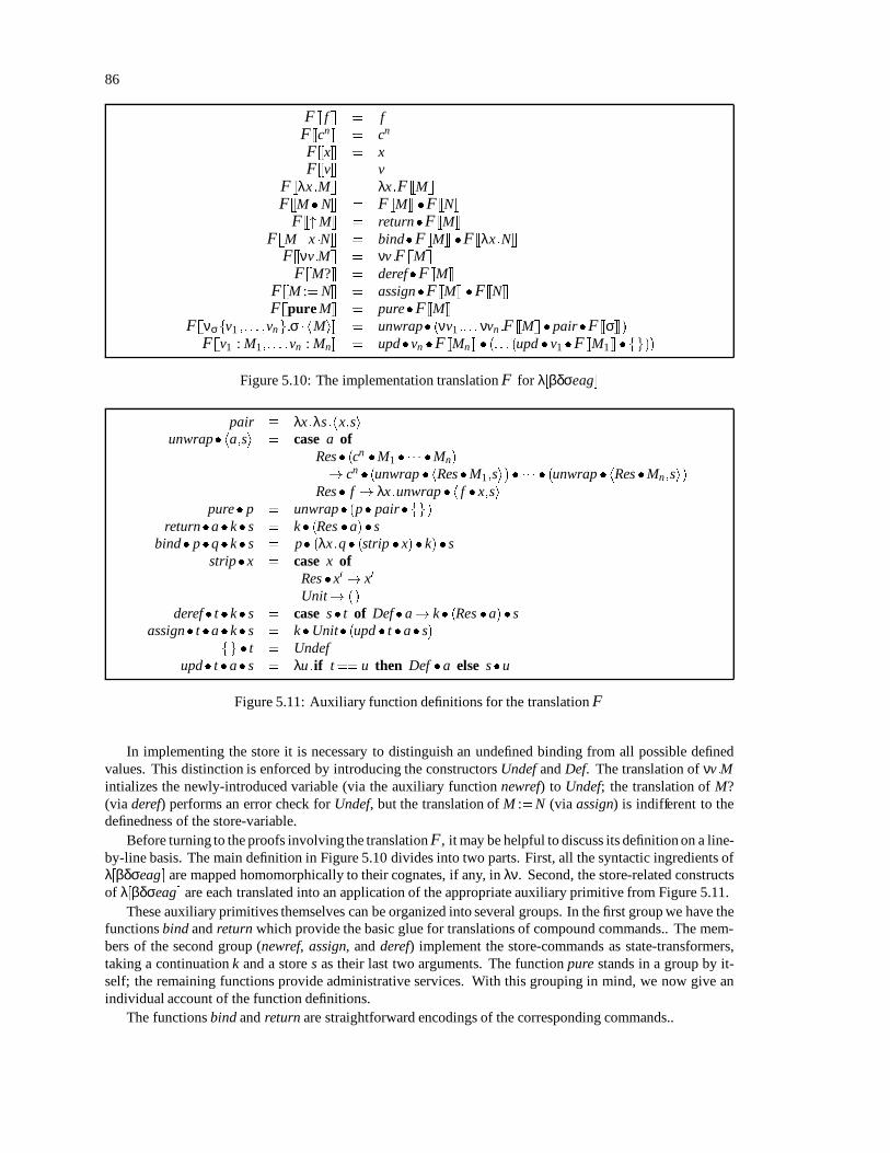
86

F [[ f ]] = fF [[cn ]] = cn

F [[x]] = xF [[v]] = v

F [[λx:M]] = λx:F [[M]]F [[MN]] = F [[M]] F [[N]]

F [["M]] = returnF [[M]]F [[M. x N]] = bindF [[M]] F [[λx:N]]

F [[νv:M]] = νv:F [[M]]F [[M?]] = derefF [[M]]

F [[M := N]] = assignF [[M]] F [[N]]F [[pure M]] = pureF [[M]]

F [[νσfv1 ;: : : ;vng:σ hMi]] = unwrap (νv1 :: : :νvn :F [[M]] pairF [[σ]])F [[v1 : M1;: : : ;vn : Mn]] = updvn F [[Mn ]] (: : : (upd v1 F [[M1 ]] fg))

Figure 5.10: The implementation translation F for λ[βδσeag]

pair λx:λs:hx;siunwrap ha;si = case a of

Res (cn M1 Mn)! cn (unwrap hResM1;si) (unwrap hRes Mn;si)

Res f ! λx:unwrap h f x;sipure p = unwrap (p pairfg)

returna k s = k (Res a) sbind pq k s = p (λx:q (strip x) k) s

stripx = case x ofRes x0 ! x0

Unit! ()deref t k s = case s t of Def a! k (Res a) s

assign t a k s = kUnit (upd t a s)fg t = Undef

upd t a s = λu:if t== u then Def a else su

Figure 5.11: Auxiliary function definitions for the translation F

In implementing the store it is necessary to distinguish an undefined binding from all possible definedvalues. This distinction is enforced by introducing the constructors Undef and Def. The translation of νv:Mintializes the newly-introduced variable (via the auxiliary function newref) to Undef; the translation of M?(via deref) performs an error check for Undef, but the translation of M :=N (via assign) is indifferent to thedefinedness of the store-variable.

Before turning to the proofs involving the translation F , it may be helpful to discuss its definition on a line-by-line basis. The main definition in Figure 5.10 divides into two parts. First, all the syntactic ingredients ofλ[βδσeag] are mapped homomorphically to their cognates, if any, in λν. Second, the store-related constructsof λ[βδσeag] are each translated into an application of the appropriate auxiliary primitive from Figure 5.11.

These auxiliary primitives themselves can be organized into several groups. In the first group we have thefunctions bind and return which provide the basic glue for translations of compound commands.. The mem-bers of the second group (newref, assign, and deref) implement the store-commands as state-transformers,taking a continuation k and a store s as their last two arguments. The function pure stands in a group by it-self; the remaining functions provide administrative services. With this grouping in mind, we now give anindividual account of the function definitions.

The functions bind and return are straightforward encodings of the corresponding commands..

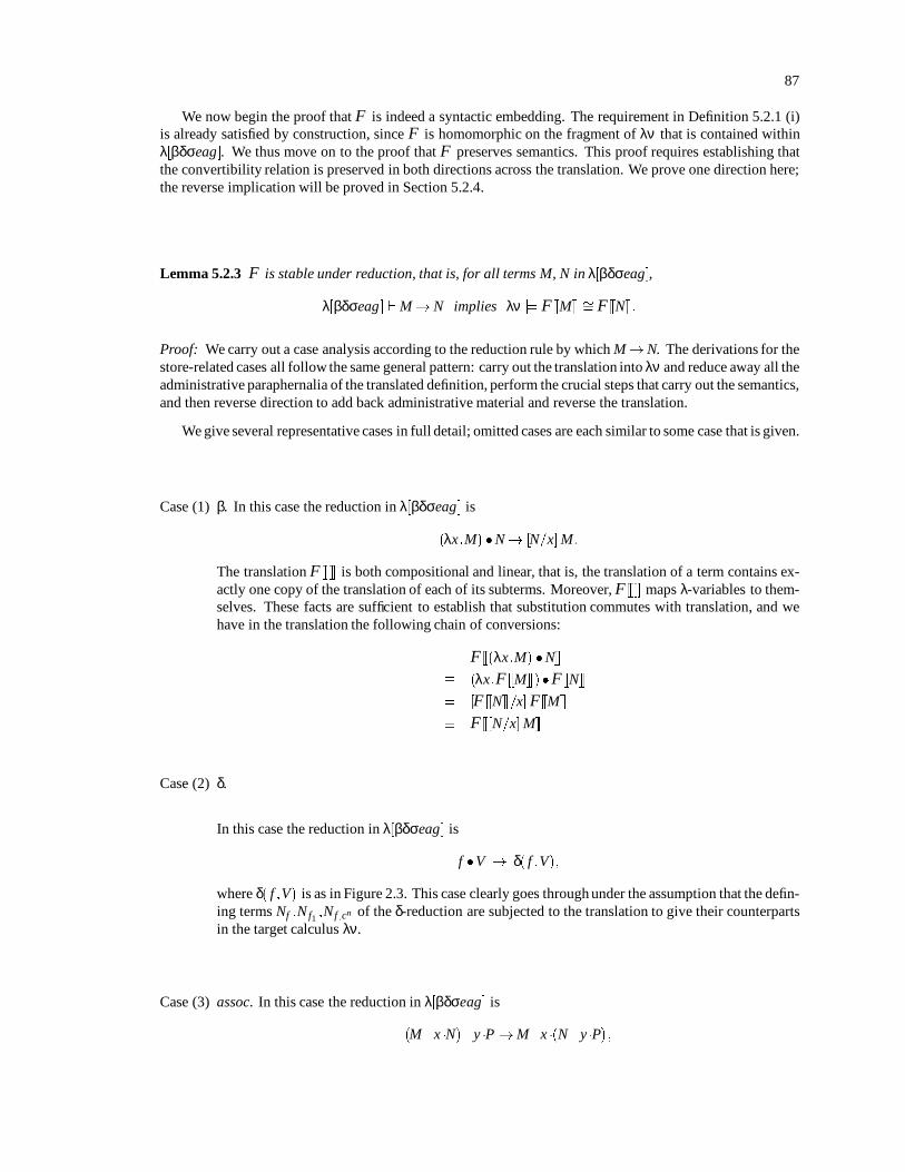
87

We now begin the proof that F is indeed a syntactic embedding. The requirement in Definition 5.2.1 (i)is already satisfied by construction, since F is homomorphic on the fragment of λν that is contained withinλ[βδσeag]. We thus move on to the proof that F preserves semantics. This proof requires establishing thatthe convertibility relation is preserved in both directions across the translation. We prove one direction here;the reverse implication will be proved in Section 5.2.4.

Lemma 5.2.3 F is stable under reduction, that is, for all terms M, N in λ[βδσeag],

λ[βδσeag] `M!N implies λν j= F [[M]] = F [[N]]:

Proof: We carry out a case analysis according to the reduction rule by which M!N. The derivations for thestore-related cases all follow the same general pattern: carry out the translation into λν and reduce away all theadministrative paraphernalia of the translated definition, perform the crucial steps that carry out the semantics,and then reverse direction to add back administrative material and reverse the translation.

We give several representative cases in full detail; omitted cases are each similar to some case that is given.

Case (1) β. In this case the reduction in λ[βδσeag] is

(λx:M) N! [N=x]M:

The translation F [[ ]] is both compositional and linear, that is, the translation of a term contains ex-actly one copy of the translation of each of its subterms. Moreover, F [[ ]] maps λ-variables to them-selves. These facts are sufficient to establish that substitution commutes with translation, and wehave in the translation the following chain of conversions:

F [[(λx:M) N]]

(λx:F [[M]])F [[N]]

= [F [[N]]=x] F [[M]]

F [[[N=x]M]]

Case (2) δ.

In this case the reduction in λ[βδσeag] is

f V ! δ( f ;V);

where δ( f ;V) is as in Figure 2.3. This case clearly goes through under the assumption that the defin-ing terms Nf ;Nf1 ;Nf ;cn of the δ-reduction are subjected to the translation to give their counterpartsin the target calculus λν.

Case (3) assoc. In this case the reduction in λ[βδσeag] is

(M. x N) .y P!M.x (N .y P);

88

and we have in the λν translation the following chain of conversions:

F [[(M. x N) .y P]] bind (bind F [[M]] (λx:F [[N]])) (λy:F [[P]])

(by definition of F)= λk:(bind F [[M]] (λx:F [[N]])) (λx0 :(λy:F [[P]]) (strip x0)k)

(by definition of bind)= λk:(λk0 :F [[M]] (λx00 :(λx:F [[N]]) (strip x00)k0)) (λx0 :(λy:F [[P]]) (strip x0) k)

(by definition of bind)= λk:F [[M]] (λx00 :(λx:F [[N]]) (strip x00) (λx0 :(λy:F [[P]]) (strip x0) k))

(by β)= λk:F [[M]] (λx00 :[(strip x00)=x]F [[N]] (λx0 :(λy:F [[P]]) (strip x0) k))

(by β)

Starting with the translation of the reduct, we have the derivation

F [[M. x (N .y P)]]= bindF [[M]] (λx:bind F [[N]] (λy:F [[P]]))

(by the definition of F)= λk:F [[M]] (λx0 :(λx:bind F [[N]] (λy:F [[P]])) (strip x0)k)

(by the definition of bind)= λk:F [[M]] (λx0 :(λx:λk:F [[N]] (λx00 :(λy:F [[P]]) (strip x00)k)) (strip x0)k)

(by the definition of bind)! λk:F [[M]] (λx0 :([(strip x0)=x] (λk:F [[N]] (λx00 :(λy:F [[P]]) (strip x00) k)))k)

(by β) λk:F [[M]] (λx0 :(λk:[(strip x0)=x]F [[N]] (λx00 :(λy:F [[P]]) (strip x00) k))k)

(because the original scope of x is N only) λk:F [[M]] (λx0 :[(strip x0)=x]F [[N]] (λx00 :(λy:F [[P]]) (strip x00) k))

(by β):

Since the two derivations reach the same term (up to α-renaming), the redex and its reduct are con-vertible (and hence operationally equivalent).

Case (4) unit.

In this case the reduction in λ[βδσeag] is

("M).x N ! [M=x]N:

Starting with the translation of the redex, we obtain the derivation

F [[("M).x N]] bind (return F [[M]]) (λx:F [[N]])

(by definition of F)! λks:(λks:k (Res F [[M]]) s) (λx0 :(λx:F [[N]]) (strip x0) k) s

(by the definitions of bind and return)! λks:(λx0 :(λx:F [[N]]) (strip x0)k) (Res F [[M]]) s

(by β)! λks:(λx:F [[N]]) (strip (Res F [[M]])) k s

(by β)! λks:(λx:F [[N]])F [[M]] k s

(by definition of strip)! λks:[F [[M]]=x]F [[N]] x s:

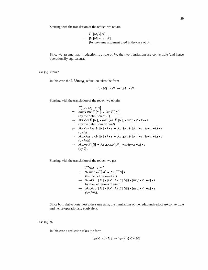
89

Starting with the translation of the reduct, we obtain

F [[[M=x]N]] [F [[M]]=x]F [[N]]

(by the same argument used in the case of β):

Since we assume that η-reduction is a rule of λν, the two translations are convertible (and henceoperationally equivalent).

Case (5) extend.

In this case the λ[βδσeag] reduction takes the form

(νv:M) .x N ! νM . x N ::

Starting with the translation of the redex, we obtain

F [[(νv:M) .x N]] bind (νv:F [[M]]) (λx:F [[N]])

(by the definition of F)! λks:(νv:F [[N]]) (λx0 :(λx:F [[N]]) stripx0 k) s

(by the definitions of bind) λks:(νv:λks:F [[N]] k s) (λx0 :(λx:F [[N]]) stripx0 k) s

(by η)! λks:(λks:νv:F [[N]] k s) (λx0 :(λx:F [[N]]) stripx0 k) s

(by λνλ)! λks:νv:F [[N]] (λx0 :(λx:F [[N]]) stripx0 k) s

(by β):

Starting with the translation of the reduct, we get

F [[νM. x N :]] νv:bind F [[M]] (λx:F [[N]])

(by the definition of F)! νv:λks:F [[M]] (λx0 :(λx:F [[N]]) (strip x0) k) s

by the definitions of bind! λks:νv:F [[M]] (λx0 :(λx:F [[N]]) (strip x0) k) s

(by λνλ):

Since both derivations meet a the same term, the translations of the redex and reduct are convertibleand hence operationally equivalent.

Case (6) σν.

In this case a reduction takes the form

νσ~v:σ hνv:Mi ! νσf~v;vg:σ hMi:

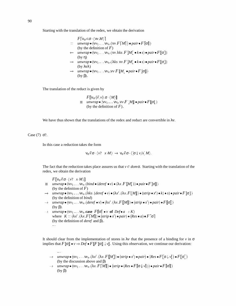
90


F [[νσ~v:σ hνv:Mi]] unwrap (νv1 :: : :νvn :(νv:F [[M]])pairF [[σ]])

(by the definition of F) unwrap (νv1 :: : :νvn :(νv:λks:F [[M]] k s)pairF [[σ]])

(by η)! unwrap (νv1 :: : :νvn :(λks:νv:F [[M]] k s)pairF [[σ]])

(by λνλ)! unwrap (νv1 :: : :νvn :νv:F [[M]] pairF [[σ]])

(by β):

The translation of the reduct is given by

F [[νσf~v;vg:σ hMi]] unwrap (νv1 :: : : νvn :νv:F [[M]] pairF [[σ]])

(by the definition of F):

We have thus shown that the translations of the redex and reduct are convertible in λν.

Case (7) σ?.

In this case a reduction takes the form

νσ~v:σ hv? .x Mi ! νσ~v:σ h[σ# v=x]Mi:

The fact that the reduction takes place assures us that v 2 domσ. Starting with the translation of theredex, we obtain the derivation

F [[νσ~v:σ hv?.x Mi]] unwrap (νv1 :: : : νvn :(bind (deref v) (λx:F [[M]]))pairF [[σ]])

(by the definition of F)! unwrap (νv1 :: : : νvn :(λks:(deref v) (λx0 :(λx:F [[M]]) (strip x0)k) s)pairF [[σ]])

(by the definition of bind)! unwrap (νv1 :: : : νvn :(deref v) (λx0 :(λx:F [[M]]) (strip x0)pair)F [[σ]])

(by β):! unwrap (νv1 :: : : νvn :case F [[σ]] v of Def a! K)

where K (λx0 :(λx:F [[M]]) (strip x0)pair) (Res a)F [[σ]](by the definition of deref and β):

It should clear from the implementation of stores in λν that the presence of a binding for v in σimplies that F [[σ]] v!Def F [[F [[σ]] # v]]. Using this observation, we continue our derivation:

! unwrap (νv1 :: : : νvn :(λx0 :(λx:F [[M]]) (strip x0)pair) (Res F [[σ# v]])F [[σ]])(by the discussion above and β)

! unwrap (νv1 :: : : νvn :(λx:F [[M]]) (strip (Res F [[σ# v]]))pairF [[σ]])(by β)

91


F [[νσ~v:σ h[σ# v=x]Mi]] unwrap (νv1 :: : : νvn :F [[[σ# v=x]M]] pairF [[σ]])

(by the definition of F) unwrap (νv1 :: : : νvn :[F [[σ# v]]=x] F [[M]] pairF [[σ]])

(by the substitutivity of F)

Case (8) σ:=. In this case the reduction in λ[βδσeag] is

νσ~v:σ hv :=N; Mi ! νσ~v:(σ ! v : N) hMi:

We show that this conversion translates into an operational equivalence via the following chain ofreasoning.

F [[νσ~v:σ hv :=N; Mi]] unwrap (νv1 :: : : νvn :(bind (assign vF [[N]]) (λz:F [[M]]))pairF [[σ]])

(by the definition of F ; z has no bound occurrences)! unwrap (νv1 :: : : νvn :(assign vF [[N]]) (λx0 :(λz:F [[M]]) (strip x0)pair)F [[σ]])

(by the definition of bind and β)! unwrap (νv1 :: : : νvn :(λx0 :(λz:F [[M]]) (strip x0)pair)Unit (upd v (Def a)F [[σ]]))

(by the definition of assign and β)! unwrap (νv1 :: : : νvn :((λz:F [[M]]) (strip Unit)pair) (upd v (Def a)F [[σ]]))

(by β)! unwrap (νv1 :: : : νvn :F [[M]] pair (upd v (Def a)F [[σ]]))

(by β, noting that z has no bound occurrences)


F [[νσ~v:(σ ! v : N) hMi]] unwrap (νv1 :: : :νvn :F [[M]] pairF [[σ ! v : N]])

(by the definition of F)

We have the desired result if we can show that

upd v (Def a)F [[σ]] = F [[σ ! v : N]]

in λν.

Case (9) σblock .

In this case the reduction takes the form

pureM ! νσfg:fg hMi:


F [[pure M]] pureF [[M]]

(by the definition of F)! unwrap (F [[M]] pairfg);

which is exactly the translation of the reduct νσfg:fg hMi.

92

Case (10) σpeag . Using the purification of an abstraction as a representative case, the reduction in λ[βδσeag]takes the form

νσ~v:σ h"λx:Mi ! λx:νσ~v:σ h"Mi:

We establish the semantic faithfulness of F in this case via the following chain of reasoning:

F [[νσ~v:σ h"λx:Mi]] unwrap (νv1 :: : : νvn :(return (λx:F [[M]]))pairF [[σ]])

(by the definition of F)! unwrap (νv1 :: : : νvn :pair Res (λx:F [[M]])F [[σ]])

(by the definition of return and β)! unwrap (νv1 :: : : νvn :hRes (λx:F [[M]]);F [[σ]]i)

(by the definition of pair)! unwrap hνv1 :: : : νvn :Res (λx:F [[M]]);νv1 :: : : νvn :F [[σ]]i

(by λνcn )! λx:unwrap hνv1 :: : : νvn :Res F [[M]];νv1 :: : :νvn :F [[σ]]i

(by the definition of unwrap, β, and δ):

The translation of the reduct is given by

F [[λx:νσ~v:σ h"Mi]] λx:unwrap (νv1 :: : :νvn :(return F [[M]])pairF [[σ]]);

from which a similar derivation leads to the last term in the derivation from the redex. This estab-lishes the convertibility of the translations.

The proofs involving the other forms of σpeag -rule are similar.


5.2.4 Reversing the translation

Lemma 5.2.3 shows that convertible terms in λ[βδσeag] are mapped by F to operationally-equivalent termsin λν. This result goes part of the way toward showing that F preserves semantics, since it shows that Fpreserves semantic equalities. However, we are also obligated to show that semantic distinctionsare preservedas well. The present section is dedicated to proving the implication in this direction.

To do so, we define a left inverse F1 for F , and show that F1 also preserves semantics in the same sensethat F does. The definition of F1 is given in Figure 5.12. Since F1 only needs to apply to λν-terms that arein the range of F , not all possible λν-terms are represented in the left-hand-sides of the defining equations forF1 . One particular nuance of the definition is that terms of the form νv:M in λν arise in two different waysas a result of F : as a translation of a λ[βδσeag] term of the form νv:M0 , or as the translation of a λ[βδσeag]term of the form σhM0i. The definition of F1 takes advantage of the detectable syntactic difference betweenthese two cases to distinguish them for the purpose of mapping them back to their original forms.

Lemma 5.2.4 (Left inverse) For all terms M in λ[βδσeag],

F1 [[F [[M]]]] M:

Proof: This proof of Lemma 5.2.4 is a straightforward induction on the structure of M; the definition in Fig-ure 5.12 does all the work.

Lemma 5.2.5 (F1 is substitutive) If M and N are terms in λν such that F1 [[M]] and F1 [[N]] are defined,then

F1 [[[N=x]M]] [F1 [[N]]=x]F1 [[M]]:

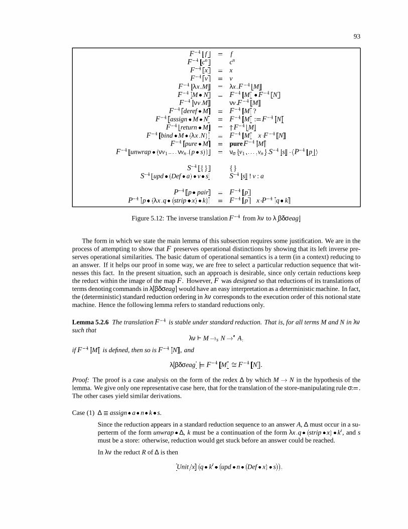
93

F1 [[ f ]] = fF1 [[cn ]] = cn

F1 [[x]] = xF1 [[v]] = v

F1 [[λx:M]] = λx:F1 [[M]]F1 [[M N]] = F1 [[M]] F1 [[N]]F1 [[νv:M]] = νv:F1 [[M]]

F1 [[deref M]] = F1 [[M]]?F1 [[assign MN]] = F1 [[M]] :=F1 [[N]]

F1 [[return M]] = "F1 [[M]]F1 [[bind M (λx:N)]] = F1 [[M]] .x F1 [[N]]

F1 [[pure M]] = pureF1 [[M]]F1 [[unwrap (νv1 :: : : νvn :(p s))]] = νσfv1 ;: : : ;vng:S1 [[s]] hP1 [[p]]i

S1 [[fg]] = fg

S1 [[upd (Def a) v s]] = S1 [[s]] ! v : a

P1 [[p pair]] = F1 [[p]]P1 [[p (λx:q (strip x) k)]] = F1 [[p]] .x P1 [[q k]]

Figure 5.12: The inverse translation F1 from λν to λ[βδσeag]

The form in which we state the main lemma of this subsection requires some justification. We are in theprocess of attempting to show that F preserves operational distinctions by showing that its left inverse pre-serves operational similarities. The basic datum of operational semantics is a term (in a context) reducing toan answer. If it helps our proof in some way, we are free to select a particular reduction sequence that wit-nesses this fact. In the present situation, such an approach is desirable, since only certain reductions keepthe reduct within the image of the map F . However, F was designed so that reductions of its translations ofterms denoting commands in λ[βδσeag] would have an easy interpretation as a deterministic machine. In fact,the (deterministic) standard reduction ordering in λν corresponds to the execution order of this notional statemachine. Hence the following lemma refers to standard reductions only.

Lemma 5.2.6 The translation F1 is stable under standard reduction. That is, for all terms M and N in λνsuch that

λν `M!s N! A;

if F1 [[M]] is defined, then so is F1 [[N]], and

λ[βδσeag] j= F1 [[M]] = F1 [[N]]:

Proof: The proof is a case analysis on the form of the redex ∆ by which M! N in the hypothesis of thelemma. We give only one representative case here, that for the translation of the store-manipulating rule σ:=.The other cases yield similar derivations.

Case (1) ∆ assignan k s.

Since the reduction appears in a standard reduction sequence to an answer A, ∆ must occur in a su-perterm of the form unwrap ∆, k must be a continuation of the form λx:q (strip x) k0, and smust be a store: otherwise, reduction would get stuck before an answer could be reached.

In λν the reduct R of ∆ is then

[Unit=x] (q k0 (upd n (Def x) s));

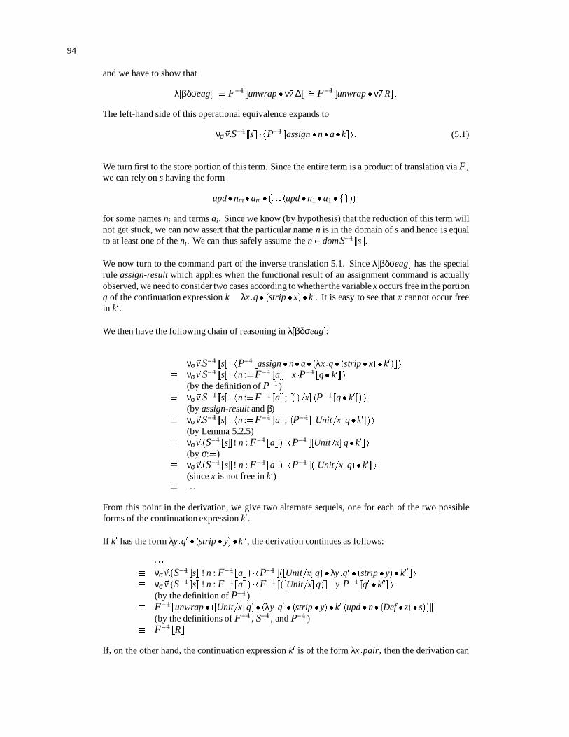
94

and we have to show that

λ[βδσeag] j= F1 [[unwrap ν~v:∆]] = F1 [[unwrap ν~v:R]]:

The left-hand side of this operational equivalence expands to

νσ~v:S1 [[s]] hP1 [[assign nak]]i: (5.1)

We turn first to the store portion of this term. Since the entire term is a product of translation via F ,we can rely on s having the form

updnm am (: : : (upd n1 a1 fg));

for some names ni and terms ai. Since we know (by hypothesis) that the reduction of this term willnot get stuck, we can now assert that the particular name n is in the domain of s and hence is equalto at least one of the ni. We can thus safely assume the n 2 domS1 [[s]].

We now turn to the command part of the inverse translation 5.1. Since λ[βδσeag] has the specialrule assign-result which applies when the functional result of an assignment command is actuallyobserved, we need to consider two cases according to whether the variable x occurs free in the portionq of the continuation expression k = λx:q (strip x) k0. It is easy to see that x cannot occur freein k0.

We then have the following chain of reasoning in λ[βδσeag]:

νσ~v:S1 [[s]] hP1 [[assign na (λx:q (strip x) k0)]]i νσ~v:S1 [[s]] hn :=F1 [[a]] .x P1 [[q k0]]i

(by the definition of P1 )= νσ~v:S1 [[s]] hn :=F1 [[a]]; [( )=x] (P1 [[q k0]])i

(by assign-result and β) νσ~v:S1 [[s]] hn :=F1 [[a]]; (P1 [[[Unit=x] qk0]])i

(by Lemma 5.2.5)= νσ~v:(S1 [[s]]! n : F1 [[a]]) hP1 [[[Unit=x] qk0]]i

(by σ:=) νσ~v:(S1 [[s]]! n : F1 [[a]]) hP1 [[([Unit=x] q) k0]]i

(since x is not free in k0)

From this point in the derivation, we give two alternate sequels, one for each of the two possibleforms of the continuation expression k0.

If k0 has the form λy:q0 (strip y)k00, the derivation continues as follows:

νσ~v:(S1 [[s]] ! n : F1 [[a]]) hP1 [[([Unit=x] q)λy:q0 (strip y) k00]]i νσ~v:(S1 [[s]] ! n : F1 [[a]]) hF1 [[([Unit=x] q)]] .y P1 [[q0 k00]]i

(by the definition of P1 ) F1 [[unwrap ([Unit=x] q) (λy:q0 (strip y) k00(upd n (Def z) s))]]

(by the definitions of F1 , S1 , and P1 ) F1 [[R]]

If, on the other hand, the continuation expression k0 is of the form λx:pair, then the derivation can

95

be continued as follows:

νσ~v:S1 [[s]] ! n : F1 [[a]] hP1 [[([Unit=x] q)pair]]i νσ~v:S1 [[s]] ! n : F1 [[a]] hP1 [[[Unit=x] q]]i

(by the definition of P1 ) F1 [[unwrap ([Unit=x] q)pair (upd n (Def a) s]]

(by the definitions of F1 and S1 ) F1 [[R]]

This concludes the proof for the case in which x occurs free in q. When x does not occur free in q,the steps in the derivation are the same except that the step involving assign-result is omitted, andthere is no need to carry along the substition of Unit for x.


5.2.5 Establishing conservative extension

We now have all the ingredients necessary to establish our desired conservative extension result. We firstobserve that we have in hand a syntactic embedding of λ[βδσeag] into λ[βδ].

Proposition 5.2.7 The translation F is a syntactic embedding of λ[βδσeag] into λ[βδ].

Proof: We first show that F preserves λ-programs. Let M be a closed λ[βδ]-term. Then by an easy inductionon the structure of M we can establish that F [[M]] M. Since there is a syntactic embedding Eν of λν intoλ[βδ], Eν [[M]] M (syntactic embeddings preserve programs). Hence the composed mapping Eσ = Eν Fpreserves programs.

We now show that Eσ preserves semantics. Since Eν is a syntactic embedding this follows from the con-dition

λ[βδσeag] `M = A if and only if λν ` F [[M]] = A

for all terms M and answers A in λ[βδσeag].We show each direction of the “if and only if” separately. First, we tackle “only if”. Assume that M = A.

Then by an induction on the length of the reduction sequence from M to A (using Lemma 5.2.3 at each step),we obtain F [[M]] = F [[A]]. But the latter term equals A by the preservation of programs.

Now we deal with “if”. Assume F [[M]] = A. Then by an induction on the length of a standard reductionfrom F [[M]] to A, we obtain F1 [[F [[M]]]] = F1 [[A]]. The right-hand side of this operational equivalenceequals A by the preservation of programs, and the left-hand side equals M by Lemma 5.2.4. Thus we obtainM = A, which is what must be proved.

Theorem 5.2.8 (Conservative extension) λ[βδσeag] is a conservative operational extension of λ[βδ]: forany two λ[βδ]-terms M, N,

λ[βδ] j= M= N if and only if λ[βδσeag] j= M = N:

Proof: By Proposition 5.2.7, there is a syntactic embedding of λ[βδσeag] into λ[βδ]. By Theorem 5.2.2, thisimplies that λ[βδσeag] is an operational extension of λ[βδ]. It remains to be shown that the extension is con-servative.

To prove this, let M and N be arbitrary terms in the common language of λ[βδ] and λ[βδσeag], and assumethat λ[βδσeag] j= M= N. By the definition of operational equivalence, this says that, for all contexts C[ ] suchthat C[M] and C[N] are closed, we have

λ[βδσeag] ` C[M] = A if and only if λ[βδσeag] ` C[N] = A:

Since this statement is true for all λ[βδσeag]-contexts, it is true for that subset which are also λ[βδ]-contexts.Restricting the statement to those contexts, and observing that M and N are λ[βδ]-terms and hence only have

96

λ[βδ]-redexes, we establish the statement

λ[βδ] ` C[M] = A if and only if λ[βδ] ` C[N] = A;

which asserts that λ[βδ] j= M= N, which was to be proved.

Corollary 5.2.9 λ[βδ!eag] is a conservative operational extension of λ[βδ]: for any two λ[βδ]-terms M, N,

λ[βδ] j= M = N if and only if λ[βδ!eag] j= M= N:

Proof: This follows immediately from Theorems 5.2.8 and 5.1.7.

5.2.6 Conservative extension for λ[βδ!laz]

Constructing a translation from λ[βδσlaz] into λ[βδ] has so far proved a severe challenge for the techniquesused in this section. The problem is not in the evaluation order itself—the resources of continuation-passingstyle are sufficient for modeling the evaluation order we require. The problem is that we have other constraints.The nesting of ν-constructs requires that later commands in a chain be lexically contained within the transla-tions of earlier commands, but the natural functional implementation of a lazy store places later commands atouter levels so that the result appears outermost and causes the execution of earlier commands by propagationof demand. We have experimented with a couple of approaches but without success so far.

5.3 Chapter summaryThis chapter has established the relationship between the operational semantics of the calculi of concern andthe operational semantics derived from consideration of store-machines. Furthermore, the results of this chap-ter show that the eager-store assignment calculus λ[βδ!eag] can be viewed as a conservative extension of abasic lambda-calculus. We conjecture that the same is true of the lazy-store calculi but we have so far hadonly partial success in constructing a proof of this fact along the lines of the proof offerred for λ[βδ!eag].

6Typed lambda-calculi with assignment

Up to this point, our presentation of lambda-calculi with assignment has been entirely in terms of untypedcalculi. We have shown that these calculi offer a suitable basis for a theory of functional programming withassignment. Nevertheless, we have several motivations for considering the construction of type systems forthese calculi:

The current standard practice in functional programming language design is to devise typed languages.

A significant precursor of our work, the Imperative Lambda Calculus of Swarup, Reddy, and Ireland[Swarup et al., 1991; Swarup, 1992] is a typed system, and the relationship to the current work hasnever been stated precisely.

The calculi λ[βδ!eag] and λ[βδ!laz] have a couple of rough edges that can be smoothed by the introduc-tion of types:

– It is possible to have runtime errors (stuck terms) resulting from attempts to read unitialized store-variables or store-variables introduced in outer pure-scopes.

– It is possible for purification to fail owing to an attempt to return an inappropriate value as theresult of a store computation.

– As discussed in Section 2.6.3, the interpretation of store-variables as locations is inhibited by theinability of the untyped calculi to guarantee that store-variable names are used only locally.

For these reasons we now turn our attention to the construction of typed versions of λ[βδ!eag] and λ[βδ!laz].We make two contributions in so doing. First (and most distressingly), the type system of Imperative LambdaCalculus, as well as the type system for λ[βδ!eag] previously proposed by Chen and Odersky [Chen and Oder-sky, 1993; Chen and Odersky, 1994], is flawed, as has been pointed out in [Huang and Reddy, 1995]. We pro-pose a new type system to correct this flaw and establish its important properties. Second, we establish thatthis type system also suffices for λ[βδ!laz].

The guiding slogan of these type systems, as for all modern polymorphic type systems, comes from Mil-ner’s seminal paper on the ML type system [Milner, 1978]: well-typed programs do not go wrong. In ourcontext, this will mean that, in addition to assuring that all function applications match the type of the actualargument to the input type of the function, and that values stored in a store-variable have the same type overtime, these type systems assure that well-typed pure expressions never get stuck.

Section 6.1 introduces the core Hindley/Milner polymorphic type system, which serves as background tothe systems considered in this chapter. Section 6.2 discusses the additional requirements imposed on a typesystem by lambda-calculi with assignments. In Section 6.3 we present the Chen/Odersky type system, bothto exhibit its known flaw and to serve as concrete introduction to the more successful type system LPJ to bepresented in Section 6.4 along with the proof of its safety for λ[βδ!eag] and λ[βδ!laz]. Section 6.5 examinesthe possibility of devising an untyped analogue of the full Launchbury/Peyton Jones typed language.

Our consideration of type systems in this chapter is confined to their safety properties only; we do notconsider the issue of implementing type-checking or type-reconstruction algorithms, or even the question ofwhether such an algorithm exists. Although it is unrealistic to proceed with a practical language design withoutknowing whether type-checking can be implemented, we exclude these subjects in order to limit the scope ofthe present investigation. There is, in fact, little reason to doubt that the type system we propose in Section 6.4possesses reasonable typing algorithms.

6.1 The Hindley/Milner polymorphic type system for functional languagesThe untyped calculi we consider have a common functional core formed by the calculus λ[βδ]. In this sectionwe present the Hindley/Milner polymorphic type system [Hindley, 1969; Milner, 1978; Damas and Milner,

97

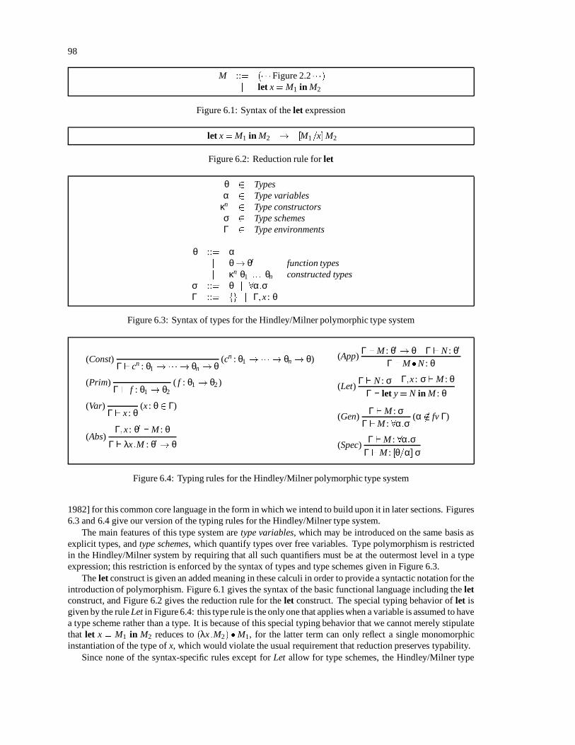
98

M ::= ( Figure 2.2 )j let x = M1 in M2

Figure 6.1: Syntax of the let expression

let x = M1 in M2 ! [M1=x]M2

Figure 6.2: Reduction rule for let

θ 2 Typesα 2 Type variables

κn 2 Type constructorsσ 2 Type schemesΓ 2 Type environments

θ ::= αj θ! θ0 function typesj κn θ1 :: : θn constructed types

σ ::= θ j 8α:σΓ ::= fg j Γ;x : θ

Figure 6.3: Syntax of types for the Hindley/Milner polymorphic type system

(Const) (cn : θ1 ! ! θn ! θ)Γ ` cn : θ1 ! ! θn ! θ

(Prim) ( f : θ1 ! θ2 )Γ ` f : θ1 ! θ2

(Var) (x : θ 2 Γ)Γ ` x : θ

Γ;x : θ0 `M : θ(Abs)

Γ ` λx:M : θ0 ! θ

Γ `M : θ0 ! θ Γ ` N : θ0(App)

Γ `MN : θ

Γ ` N : σ Γ;x : σ `M : θ(Let)

Γ ` let y = N in M : θ

Γ `M : σ(Gen) (α 62 fv Γ)

Γ `M : 8α:σ

Γ `M : 8α:σ(Spec)

Γ `M : [θ=α] σ

Figure 6.4: Typing rules for the Hindley/Milner polymorphic type system

1982] for this common core language in the form in which we intend to build upon it in later sections. Figures6.3 and 6.4 give our version of the typing rules for the Hindley/Milner type system.

The main features of this type system are type variables, which may be introduced on the same basis asexplicit types, and type schemes, which quantify types over free variables. Type polymorphism is restrictedin the Hindley/Milner system by requiring that all such quantifiers must be at the outermost level in a typeexpression; this restriction is enforced by the syntax of types and type schemes given in Figure 6.3.

The let construct is given an added meaning in these calculi in order to provide a syntactic notation for theintroduction of polymorphism. Figure 6.1 gives the syntax of the basic functional language including the letconstruct, and Figure 6.2 gives the reduction rule for the let construct. The special typing behavior of let isgiven by the rule Let in Figure 6.4: this type rule is the only one that applies when a variable is assumed to havea type scheme rather than a type. It is because of this special typing behavior that we cannot merely stipulatethat let x = M1 in M2 reduces to (λx:M2) M1, for the latter term can only reflect a single monomorphicinstantiation of the type of x, which would violate the usual requirement that reduction preserves typability.

Since none of the syntax-specific rules except for Let allow for type schemes, the Hindley/Milner type

99

Γ `M : θ(Weaken)

Γ;x : θ0 `M : θ:: : ;x1 : σ1 ;: : : ;x2 : σ2 ;: : : `M : θ

(Permute):: : ;x2 : σ2 ;: : : ;x1 : σ1 ;: : : `M : θ

Figure 6.5: Structural rules for type derivations

system provides a way of introducing and eliminating type schemes by using the rules Gen and Spec. The ruleGen allows the introductionof a schematic variable α provided that no type assumed in the type environment Γhas a free occurrence of α. Informally, this side conditionmeans that the type judgment Γ `M : σ is indifferentas to what actual type that may be represented by the type variable α. The rule Spec expresses the inverseprocess of instantiating a type scheme with any particular type. Informally, since the type scheme could onlyhave been established by indifference as to the actual type to take the place of α, this specialization ought tobe safe. The following type derivation of a polymorphic type for a use of the identity function illustrates theuse of these rules:

(Var)x : α ` x : α

(Abs)` λx:x : α! α

(Gen)` λx:x : 8α:α! α(Spec)` λx:x : Int! Int

(Const)` 1 : Int

(App)` (λx:x) 1: Int .

One feature of our presentation of the Hindley/Milner type system is not present in Milner’s paper, but isadopted following present practice (including [Chen and Odersky, 1994]): we assume the existence of typeconstructors κn of arity n. These type constructors are useful in typing the value constructors of the basiccalculus. For example, if our lambda-calculus contains a constructor pair of arity 2, we may wish to posita constructed type Pair such that pair has type 8α:8β:α ! β! Pair α β. Since value-constructors in ourbasic lambda-calculi subsume constants, the introduction of type-constructors also serves to define types ofconstants, such as the type of the integers, as nullary type constructors.

In addition to constructed types, the basic type system in Figure 6.4 provides a rule that assigns a pre-determined type to primitive function names. In order for the type system to prevent well-typed terms fromgetting stuck, we must assume that these primitive functions are defined on all arguments of their argumenttype, where f being defined on an argument V means that f V is a δ-redex. In terms of types, we assume thatfor every primitive function f with type τ1 ! τ2 and every value-constructor cn such that cn M1 Mn hastype τ1 , f (cn M1 Mn) is defined and has type τ2 . We make a similar assumption for primitives thattake functional arguments: if ` f : (τ1 ! τ2 )! τ3 and ` λx:M : τ1 ! τ2 , then f (λx:M) is a redex; likewisefor ` f 0 : τ1 ! τ2 and f f 0 . In addition to forming the base case of type safety for our functional program-ming languages, these restrictions eliminate the possibility for such pathological primitive function types as8α:8β:α! β because there is no way to generalize to such polymorphic types from the concrete definingapplication terms that we are required to provide for each primitive function. The typing of constructors isspecified by type axioms of the same form as those for primitive functions.

Our reasoning with type derivations in this chapter will make use of additional rules, called structural rules,given in Figure 6.5. The rule Weaken allows us to add irrelevant type assignments to an assumption withoutdisturbing the conclusion; the rule Permute lets us reorder the type assignments within a type environment atwill. These rules are actually theorems of the given type systems; properly stated, they give us the existenceof a derivation for the conclusion from a derivation of the premise. These theorems are established by induc-tion over the structure of type derivations. We omit the details, but we note for example that for Weaken theaxiom Var forms the interesting base case, and that the induction steps typically work because weakened typeassumptions on the subterms are just carried through from the premises to the conclusions of the rules.

The safety of the Hindley/Milner type system rests on the assumption that the primitive functions do not gowrong on arguments of the correct type: this means that when they terminate, they really do produce as resultsterms having the types implied by their declarations. In our calculus, which has multistep δ-rules, we actuallyneed the stronger assumption that every δ-rewriting preserves types; this is a condition on the the constant

100

terms Nf and so forth that appear in the definitions of primitive functions. The proof of soundness is essen-tially an induction on reductions showing that well-typed terms not only contain no applications of primitivefunctions to expressions of inappropriate type but also can never produce such an application by reduction.The key component of this proof is the proof of subject reduction, the property that any type derivable for aterm is also derivable for any of its reducts. The contrapositive statement of this property is that the antecedentof an ill-typed term must also have been ill-typed; there is therefore no way to arrive at an ill-typed primitiveapplication from a well-typed starting term.

A key part of a proof of subject reduction, in turn, is a substitutivity lemma establishing that the β-rulepreserves well-typing. In the basic functional programming language with only the β- and δ-rules this is almostthe whole of subject reduction, but in the treatment of our extended calculi to follow we have many additionalcases to consider.

One further aspect of the Hindley/Milner type system is noteworthy for the developments in this chap-ter: it works equally well for call-by-name and call-by-value versions of the underlying lambda-calculus. In-formally, this property may be understood as deriving from the fact that the type system infers the possibleconsequences of an application based on approximate information that does not capture the time of reduction.Formally, the soundness result for the call-by-name calculus is a consequence of soundess for call-by-value bythe following reasoning: Every call-by-value β-redex is also a call-by-name β-redex, therefore a stuck termin the call-by-name calculus is also stuck in the call-by-value calculus. The type system is sound for call-by-value, therefore the term in question must be ill-typed, a property that is independent of the evaluation orderof the calculus. Thus a stuck call-by-name term is ill-typed. This establishes soundness for the call-by-namecalculus. This form of reasoning depends on establishing the subject-reduction property for both calculi.

6.2 What should a type system for a lambda-calculus with assignments do?The assignment constructs that we have added to the basic lambda-calculus present several new challenges fora type system. The most important of these, and the most complex to address, is to assure that the purificationof the result of a store-computation never becomes stuck. Encountering a stuck purification in the calculuscorresponds informally to an attempt to export observation of a store outside its lifetime; only terms that canbe interpreted independently of a particular store can be purified in the calculus.1

Besides assuring that purification of well-typed terms always proceeds to completion, a type system forlambda-calculi with assignment can also ease a couple of less important nuisances present in the untyped cal-culi. As discussed in Chapter 2, the untyped calculi cannot enforce a requirement that store-variables involvedin a particular store-computation are local to that computation. This shortcoming prevents us from interpret-ing the name of a store-variable as a particular location in which a value is stored because it only becomesmeaningful to speak of a location with respect to a particular store. If non-local names can be used to accessa store, the interpretation of such a name must be associated with the point of use, not the point of definition.

A type system typically performs a static analysis that approximates a dynamic behavior of a program. Inthe basic Hindley-Milner type system, this analysis tracks which types of values might be supplied to prim-itives through all the twists and turns of lambda-abstractions and applications; a type system for a lambda-calculus with assignment ought correspondingly to track locality of declaration for uses of store-variables.We will see below that this analysis can be carried out in a straightforward fashion.

With a type system to enforce that only locally-declared store-variables affect a store-computation, it ispossible to restore our originally-intended semantics identifying store-variables with locations: now there isonly one store relevant for the interpretation of such names.

6.3 The Chen/Odersky type system for λ[βδ!eag] and λ[βδ!laz]

The type system of Chen and Odersky (given both in [Chen and Odersky, 1993] and in [Chen and Odersky,1994]) was proposed to provide a sound typing mechanism for λvar , the predecessor of λ[βδ!eag]. Many of the

1But not nearly all such independently-meaningful terms can be purified in λ[βδ!eag] and λ[βδ!laz ]. The language-feature designproposed by Launchbury and Peyton Jones [Launchbury and Peyton Jones, 1994] allows far more such terms than our present calculi;we discuss the difficulties of modeling their proposal as a lambda-calculus with assignment in Section 6.5.

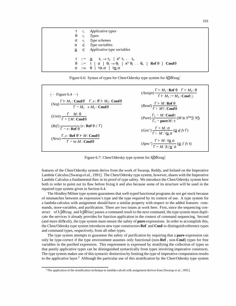
101

τ 2 Applicative typesθ 2 Typesσ 2 Type schemesα 2 Type variablesα 2 Applicative type variables

τ ::= α j τ1 ! τ2 j κn τ1 :: : τn

θ ::= τ j α j θ1 ! θ2 j κn θ1 :: : θn j Ref θ j Cmdθσ ::= θ j 8α:σ j 8α:σ

Figure 6.6: Syntax of types for Chen/Odersky type system for λ[βδ!eag]

( Figure 6.4 )

Γ `M1 : Cmdθ0 Γ;x : θ0 `M2 : Cmdθ(Seq)

Γ `M1 .x M2 : Cmdθ

Γ `M : θ(Unit)Γ ` "M : Cmdθ

(Ref ) (v : Ref θ 2 Γ)Γ ` v : Ref θ

Γ;v : Ref θ0 `M : Cmdθ(New)

Γ ` νv:M : Cmdθ

Γ `M1 : Ref θ Γ `M2 : θ(Assign)

Γ `M1 :=M2 : Cmd ()

Γ `M : Ref θ(Read)

Γ `M?: Cmdθ

Γτ `M : Cmdτ(Pure) (M Slaz["N])

Γτ ` pureM : τ

Γ `M : σ(Gen’) (α 62 fv Γ)Γ `M : 8α:σ

Γ `M : 8α:σ(Spec’) (α 62 fv τ)

Γ `M : [τ=α]σ

Figure 6.7: Chen/Odersky type system for λ[βδ!eag]

features of the Chen/Odersky system derive from the work of Swarup, Reddy, and Ireland on the ImperativeLambda Calculus [Swarup et al., 1991]. The Chen/Odersky type system, however, shares with the ImperativeLambda Calculus a fundamental flaw in its proof of type safety. We introduce the Chen/Odersky system hereboth in order to point out its flaw before fixing it and also because some of its structure will be used in therepaired type system given in Section 6.4.

The Hindley/Milner type system guarantees that well-typed functional programs do not get stuck becauseof mismatches between an expression’s type and the type required by its context of use. A type system fora lambda-calculus with assignment should have a similar property with respect to the added features: com-mands, store-variables, and purification. There are two issues at work here. First, since the sequencing con-struct . of λ[βδ!eag] and λ[βδ!laz] passes a command result to the next command, the type system must dupli-cate the services it already provides for function application in the context of command sequencing. Second(and more difficult), the type system must ensure the safety of pure-expressions. In order to accomplish this,the Chen/Odersky type system introduces new type constructors Ref and Cmd to distinguish reference typesand command types, respectively, from all other types.

The type system attempts to guarantee the safety of purification by requiring that a pure-expression canonly be type-correct if the type environment assumes only functional (non-Ref , non-Cmd) types for freevariables in the purified expression. This requirement is expressed by stratifying the collection of types sothat purely applicative types can be distinguished syntactically from types involving imperative constructs.The type system makes use of this syntactic distinction by limiting the type of imperative computation resultsto the applicative layer.2 Although the particular use of this stratification by the Chen/Odersky type system

2The application of the stratification technique to lambda-calculi with assignment derives from [Swarup et al., 1991].

102

is insufficient to achieve its goal of assuring the safety of attempted purifications, the basic stratified structureworks and is retained in the type system LPJwhich we will introduce in Section 6.4.

The syntax of type expressions in the Chen/Oderskysystem is given in Figure 6.6, and the additional typingrules are given in Figure 6.7.

Several features of this type system require special comment. First, it is assumed that there are no con-stants of reference or command type, nor are there primitive functions involving such types (except perhapsas projections from constructed types). Second, the types in Figure 6.6 incorporate a special class of type vari-ables that are only capable of being instantiated by types in the applicative layer. Corresponding to this classof type variables are special versions of the typing rules Gen and Spec. Third, the rule Pure requires that thetypes assumed for every variable in the type environment be restricted to the applicative layer. This restrictionis notated by annotating the meta-symbol for type environments with a subscript τ. Rule Pure also requiresthat the result type of the command be an applicative type. The side condition M Slaz["N] on rule Pure isintended by Chen and Odersky to assure that the pure-expression returns some value.3 It should be noted thatthe restriction in question is very easily satisfied by writing pureM .x " x instead of pureM if M does nothave the required form; it is not clear that the restriction is really required, but it is certainly harmless.

It is in fact the formulation of the rule Pure that trips up the Chen/Odersky type system. As we discussed inSection 6.1, the property of subject reduction is a crucial step in establishing the soundness of a type systemaccording to standard proof techniques; it is subject reduction that fails for the Chen/Odersky system. Theculprit in this failure is the restriction in the rule Pure, which requires a type environment that assumes only τtypes. Unfortunately, the set of free variables that must be assigned in such an environment is subject to changeupon substitution during a β-reduction. This issue can be traced as far back as the work of Reynolds on thesyntactic control of interference [Reynolds, 1978], as pointed out in the introductory sections of [O’Hearnet al., 1995].

The following counterexample to the Chen/Odersky is similar to those given in the literature on syntacticcontrol of interference; we have adapted it to the syntax of λ[βδ!eag]. We consider the term

pureνw:w := 2; "((λx:pure "x) (fst h1;wi));

which can be given a type derivation as follows. We present first a subtree of the type derivation in consid-eration of our limited page width. This subtree is presented for completeness only; the interesting part of thederivation follows afterwards.

` fst : 8α:8β:hα;βi ! α

w : Ref Int;z : () ` fst : hInt;Ref Inti ! Int w : Ref Int;z : () ` h1;wi : hInt;Ref Inti

w : Ref Int;z : () ` fsth1;wi : Int ; (6.1)

The interesting part of the type derivation is the following:

w : Ref Int ` w :=2 : Cmd()

x : Int ` x : Intx : Int ` "x : CmdInt

x : Int ` pure"x : Int

w : Ref Int;z : () ` λx:pure "x : Int! Int (6.1)

w : Ref Int;z : () ` ((λx:pure "x) (fst h1;wi)) : Int

w : Ref Int;z : () ` " ((λx:pure "x) (fst h1;wi)) : CmdInt

w : Ref Int ` w :=2; "((λx:pure "x) (fst h1;wi)) : Cmd Int

` νw:w := 2; " ((λx:pure "x) (fst h1;wi)) : CmdInt

` pureνw:w := 2; "((λx:pure "x) (fst h1;wi)) : Int .

3The definition of Slaz[] is given in Figure 2.11. It is used here as a handy syntactic abbreviation—its role in the statement of the rule

has nothing to do with laziness.

103

Note that the inner pure-expression is judged typable in a type environment containing a type assignment onlyfor the free lambda-bound variable x. The assumption is that x has type Int, which is an applicative type, sothe side condition is satisfied.

Now let us carry out the β-reduction, obtaining the term

pureνw:w := 2; "pure"(fst h1;wi):

If we try to construct a type derivation for this term, we run into trouble: the inner pure-expression now con-tains a free occurrence of the store-variable w, which must be accounted for in the type environment present inthe application of rule Pure. The side condition will thus be violated, since the type of w is constrained by itsorigin in the outer pure to have type Ref Int. The β-reduction step has caused a loss of typability, and hencesubject reduction does not hold for the Chen/Odersky type system.

The rather fussy subterm fsth1;wi appearing in this counterexample may appear puzzling, but this con-struction is necessary in order to pin the blame on the side condition rather than on the condition that the resulttype of the pure-expression belongs to the applicative layer. Putting the offending store-variable into the ig-nored slot of a projection from a product type runs afoul of the side condition (because all free variables mustbe assigned types in the type environment, and hence must be assigned applicative types) but satisfies theresult-type condition (because the type of w is, in fact, ignored).

This counterexample to subject reduction actually only invalidates a proof technique for type soundness;its existence does not necessarily disprove type soundness itself. In fact, the counterexample given reducessuccessfully to the answer 1. When a proof technique fails without suggesting that the theorem itself is false,we are faced with a choice between finding another proof technique for establishing the same theorem or mod-ifying the theorem. In our repair of the situation in Section 6.4 we will modify the theorem by considering adifferent type system that is not sensitive to the changes in free-variable sets that come with substitution. Werationalize that subject reduction is more than just a proof technique—it is intimately tied to our informal un-derstanding that a program denotes a value and that that value has an unchanging type.

Uninitialized store-variables

One technical detail of [Chen and Odersky, 1994] that we will treat differently here has to do with the wayin which errors due to uninitialized store-variable are dealt with. Chen and Odersky introduce a reductionνv:v? .x P ! νv:v? .x P in order to make such terms diverge rather than get stuck, since the type systemdoes not, in fact, prohibit them. As a matter of taste, we choose instead to stipulate that all store-variables areinitialized immediately upon declaration (as in νv:v := M; P), and that the check for this restriction is madeindependently of the type system (perhaps by modifying the syntax of the language).

This solution to the unitialized-variableproblem creates a minor secondary problem: the original reductionrules in Figures 2.7 and 2.9 allow the creation of intermediate forms that do not satisfy our stipulation that allallocated store-variables be immediately initialized. In particular, the rule bubble-assign can bubble a store-variable read into the position between the allocation and the initialization, as in the reduction

νv:v := M1; w?.x2 M2 ! νv:w? .x2 v := M1; M2! w?.x2 νv:v := M1; M2:

The way out of this minor dilemma is to note that, if the first reduction above is permitted by virtue of v andw being distinct store-variables, then so is the second. In fact, a standard reduction will perform these re-ductions consecutively or not at all, so the condition that the declaration of a store-variable must be followedimmediately by an initial assignment to it is already maintained by the reduction semantics.

Another minor issue arising from our insistence that store-variables be immediately initialized is that build-ing certain recursive store structures becomes awkward. For example, it is perfectly reasonable in an untypedcalculus to set up two store variables having each other as assigned values, as in

νv:νw:v := w; w :=v:

It should be noted, however, that this term can have no finite type, because the reference type of each of v

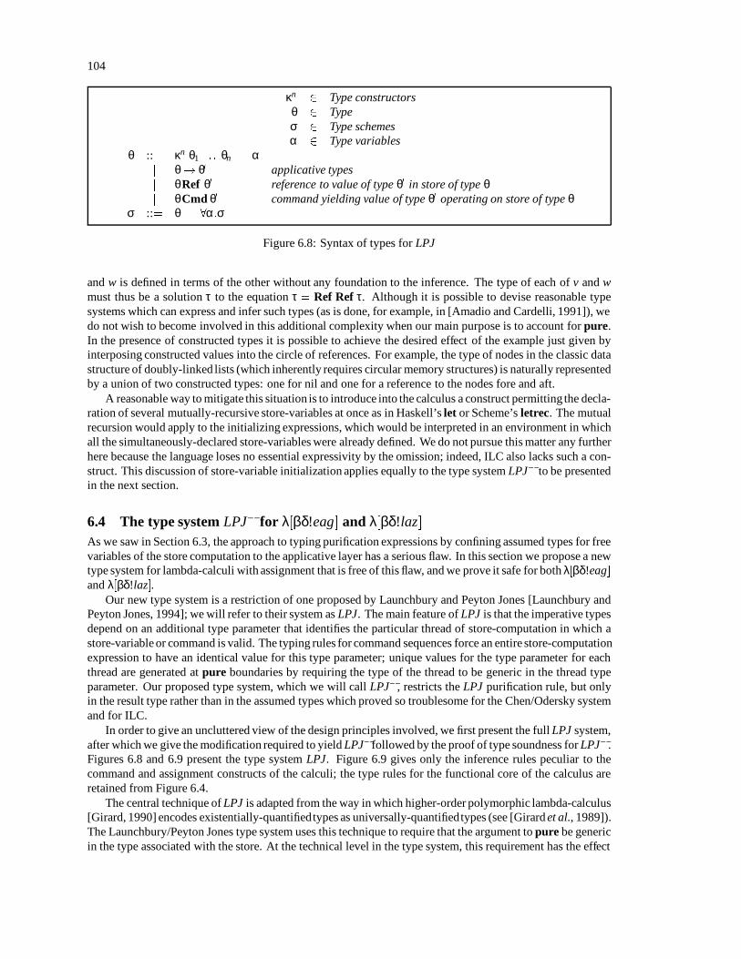
104

κn 2 Type constructorsθ 2 Typeσ 2 Type schemesα 2 Type variables

θ ::= κn θ1 :: : θn j αj θ! θ0 applicative typesj θRef θ0 reference to value of type θ0 in store of type θj θCmd θ0 command yielding value of type θ0 operating on store of type θ

σ ::= θ j 8α:σ

Figure 6.8: Syntax of types for LPJ

and w is defined in terms of the other without any foundation to the inference. The type of each of v and wmust thus be a solution τ to the equation τ = Ref Ref τ. Although it is possible to devise reasonable typesystems which can express and infer such types (as is done, for example, in [Amadio and Cardelli, 1991]), wedo not wish to become involved in this additional complexity when our main purpose is to account for pure.In the presence of constructed types it is possible to achieve the desired effect of the example just given byinterposing constructed values into the circle of references. For example, the type of nodes in the classic datastructure of doubly-linked lists (which inherently requires circular memory structures) is naturally representedby a union of two constructed types: one for nil and one for a reference to the nodes fore and aft.

A reasonable way to mitigate this situation is to introduce into the calculus a construct permitting the decla-ration of several mutually-recursive store-variables at once as in Haskell’s let or Scheme’s letrec. The mutualrecursion would apply to the initializing expressions, which would be interpreted in an environment in whichall the simultaneously-declared store-variables were already defined. We do not pursue this matter any furtherhere because the language loses no essential expressivity by the omission; indeed, ILC also lacks such a con-struct. This discussion of store-variable initialization applies equally to the type system LPJ to be presentedin the next section.

6.4 The type system LPJ for λ[βδ!eag] and λ[βδ!laz]

As we saw in Section 6.3, the approach to typing purification expressions by confining assumed types for freevariables of the store computation to the applicative layer has a serious flaw. In this section we propose a newtype system for lambda-calculi with assignment that is free of this flaw, and we prove it safe for both λ[βδ!eag]and λ[βδ!laz].

Our new type system is a restriction of one proposed by Launchbury and Peyton Jones [Launchbury andPeyton Jones, 1994]; we will refer to their system as LPJ. The main feature of LPJ is that the imperative typesdepend on an additional type parameter that identifies the particular thread of store-computation in which astore-variable or command is valid. The typing rules for command sequences force an entire store-computationexpression to have an identical value for this type parameter; unique values for the type parameter for eachthread are generated at pure boundaries by requiring the type of the thread to be generic in the thread typeparameter. Our proposed type system, which we will call LPJ, restricts the LPJ purification rule, but onlyin the result type rather than in the assumed types which proved so troublesome for the Chen/Odersky systemand for ILC.

In order to give an uncluttered view of the design principles involved, we first present the full LPJ system,after which we give the modification required to yield LPJfollowed by the proof of type soundness for LPJ.Figures 6.8 and 6.9 present the type system LPJ. Figure 6.9 gives only the inference rules peculiar to thecommand and assignment constructs of the calculi; the type rules for the functional core of the calculus areretained from Figure 6.4.

The central technique of LPJ is adapted from the way in which higher-order polymorphic lambda-calculus[Girard, 1990] encodes existentially-quantifiedtypes as universally-quantifiedtypes (see [Girard et al., 1989]).The Launchbury/Peyton Jones type system uses this technique to require that the argument to pure be genericin the type associated with the store. At the technical level in the type system, this requirement has the effect

105

Γ `M1 : θCmd θ0 Γ;x : θ0 `M2 : θCmd θ00(Seq)

Γ `M1 .x M2 : θCmd θ00

Γ `M : θ0(Unit)Γ ` "M : θCmd θ0

(Ref ) (v : θRef θ0 2 Γ)Γ ` v : θRef θ0

Γ;v : θRef θ0 `M : θCmd θ00(New)

Γ ` νv:M : θCmd θ00

Γ `M : θRef θ0(Read)

Γ `M?: θCmd θ0

Γ `M1 : θRef θ0 Γ `M2 : θ0(Assign)

Γ `M1 :=M2 : θCmd ()

Γ `M : 8α:α Cmd θ(Pure) (

α 62 fv θ;M Slaz["N]

)Γ ` pureM : θ

Figure 6.9: Type inference rules for LPJ

of requiring that the type variable be absent from the type of the returned value of the pure. Since occurrencesof the type variable correspond to occurrences of the store, the purified value must be free of references to thatparticular thread. This device goes beyond the level of polymorphism present in the Hindley/Milner, since iteffectively gives the pure operator the type scheme 8β:(8α:α Cmd β)! β, which does not have all its quan-tifiers at the outermost level, but Launchbury and Peyton Jones argue that the negative consequences of thisminor foray into second-order polymorphism are minimal.

Figure 6.8 gives the syntax of LPJ type expressions. There are two major contrasts to the Chen/Oderskysystem to be noted. First, there is only one stratum and one kind of type variable. Second, the imperative typeconstructors take an extra parameter, which we write before the keyword as in θ1 Ref θ2 and θ1 Cmd θ2 .4

This extra parameter is the unique type of the store thread in which the reference or command is valid; inexpressions of applicative type it will always be a type variable.

The type rules of LPJ are given in Figure 6.9. These rules all follow the same pattern as the correspondingChen/Odersky rules, with two exceptions. First, the rules for typing compound commands carry along the newstore-thread types and require that they match. Second, the purification rule Pure implements the trick alludedto above: a command can only be purified if its type is generic in the store-thread type that must be matched byevery component of the command. Note that this does not prohibit the presence of a different store-thread typeas a component of the result type τ as the Chen/Odersky system would. This leniency is a major contributionof the Launchbury/Peyton Jones type system.

Unfortunately, it is precisely this leniency that prohibitsus from usingLPJ as a substitutefor the Chen/Oder-sky system. Our untyped calculi do not under any circumstances permit a command or store-variable to bethe result of a store-computation, so LPJ is necessarily unsound for λ[βδ!eag] and λ[βδ!laz]. We clearly needto restrict the LPJ rule Pure so that these types of constructs will never be considered for purification.5

Our solution is to construct a hybrid of LPJ with the stratified type structure characteristic of ILC andthe Chen/Odersky type system. Figure 6.10 gives the syntax of types for the hybrid type system LPJ. Theapplicative types are denoted by τ, the more general types including the store-variable and command types byθ, and a special class of types specific to the purification rule by ψ. The ψ types are exactly the types of theconstructs that can be completely purified by the reduction rules pure-eager and pure-lazy; the modified Purerule given in Figure 6.11 restricts the type inferred for the result of the command sequence to be purified to ψtypes. Aside from this restriction, LPJ is just LPJ.

The safety provided by LPJ is a matter for the proofs to follow, but we first note that the problem raisedby the counterexample given in Section 6.3 is not present, because we have no condition on the free variablesof the store-computation’s result expression, but only on its type (which must be a ψ type). We have taken ad-vantage of an informal parametricity property of our type system: the type of an input that actually contributes

4We adopt this infix notation (which is ours) in order to reduce the need for parentheses that arise with the use of the usual style ofprefix placement of the type constructor. We cite the function-type constructor as a precedent.

5It is certainly possible to attempt to allow the LPJ type system’s attractive leniency to influence the design of an untyped lambda-calculus with assignment with respect to which LPJ can be proved sound. We report on difficulties with this attempt in Section 6.5.

106

κ 2 Type constructorsτ 2 Applicative typesθ 2 Typesψ 2 OK typesσ 2 Type schemesα 2 Applicative type variablesα 2 Type variables

τ ::= κn τ1 :: : τn j αj τ! τ0 applicative types

θ ::= α j τ j θ! θ0j κn θ1 :: : θn

j τRef τ0 reference to value of type τ0 in store of type τj τCmd τ0 command yielding value of type τ0 operating on store of type τ

ψ ::= τ j θ! ψj κn ψ1 :: : ψn

σ ::= τ j 8α:σ j 8α:σ

Figure 6.10: Syntax of types for LPJ

Γ `M : 8α:α Cmd ψ(Pure) (

α 62 fv ψ;M Slaz["N]

)Γ ` pureM : ψ

Figure 6.11: Modified inference rule for LPJ

Γ `M : σ(Gen’) (α 62 fv Γ)

Γ `M : 8α:σ

Γ `M : 8α:σ(Spec’) (α 62 fv τ)

Γ `M : [τ=α]σ

Figure 6.12: Additional rules for LPJ

to the output must be reflected in the output type.We now begin the proof that LPJ is safe for λ[βδ!eag] and λ[βδ!laz]. We first prove the substitutiv-

ity lemma that supports the β-reduction case in the proof of subject reduction. We formulate the lemma interms of type schemes both because it makes a better induction hypothesis and because we need to take let-polymorphism into account.

Lemma 6.4.1 (Substitutivity) In LPJ, if Γ;x : σ1 `M1 : σ2 and Γ `M2 : σ1 , then Γ ` [M2=x]M1 : σ2 .

Proof: We carry out an inductionon the structure of the type derivation for the hypothesised judgmentΓ;x : σ1 `

M1 : σ2 .The only interesting base case is M1 x, in which case [M2=x]M1 M2 and the lemma follows from the

hypothesis Γ `M2 : σ1 . In all the other base cases (M1 v, M1 y 6 x, M1 f , M1 c0) the lemma is easilyseen to hold: no substitution actually takes place. In these cases there is no occurrence of x in M1, and thedesired conclusion follows from the hypotheses by omitting the irrelevant type assignment for x from the typejudgment.

We take as inductionhypothesis the statement of the lemma, but withM1 restricted to terms of lower heightthan the term under consideration.

Case (1) Rule App: M1 N1 N2 .

In this case the assumed typing for M1 must be supported by an inference tree of the form

107

Γ;x : σ1 ` N1 : θ3 ! θ2 Γ;x : σ1 ` N2 : θ3

Γ;x : σ1 ` N1 N2 : θ2 .

The assumptions that we are forced to make in this type derivation, along with the induction hy-pothesis, are sufficient to establish Γ ` [M2=x]N1 : θ3 ! θ2 and Γ ` [M2=x]N2 : θ2 . We use thesetype judgments as assumptions in the following type derivation, which establishes the lemma in thiscase:

Γ ` [M2=x]N1 : θ3 ! θ2 Γ ` [M2=x]N2 : θ2

Γ ` [M2=x] N1 [M2=x]N2( [M2=x]N2 N2) : θ2 .

Case (2) Rule Abs: M1 λy:N.

In this case we must have a type derivation of the form

Γ;x : σ1 ;y : θ3 ` N : θ4

Γ;x : σ1 ` λy:N : (θ3 ! θ4)( θ2).

The assumption of this derivation together with the induction hypothesis then gives the assumptionof the following type derivation, which establishes the lemma in this case. The only twist is that wehave used the fact that the type assignments within type environments may be permuted:

Γ;y : θ3 ` [M2=x]N : θ4

Γ ` λy:[M2=x]N( [M2=x] (λy:N)) : (θ3 ! θ4)( θ2).

This pattern of proof requires only the fact that substitution commutes with term-construction. Therest of the cases based on type rules for syntactic constructs follow this pattern; we treat the case forrule Pure in full because of the presence of the condition on the result type.

Case (3) Rule Gen:

In this case, we have a type derivation of the form

Γ;x : σ1 `M1 : σ2(α 62 fv Γ;x : σ1 )

Γ;x : σ1 `M1 : 8α:σ2 .

The induction hypothesis (recall that the induction is over the structure of type derivations, not thatof terms) gives us the existence of a derivation of the judgment Γ ` [M2=x]M1 : σ2 . Now if thetype variable α is not free in the type environment Γ;x : σ1 , it certainly cannot be free in the strictlysmaller type environment Γ. Hence the side condition for rule Gen is satisfied, and we can inferΓ `M1 : 8α:σ2 by rule Gen.

Case (4) Rule Spec:

In this case the root node of our given type derivation takes the form

Γ;x : σ1 `M : 8α:σ3(α 62 fv θ3 )

Γ;x : σ1 `M : [θ3=α]σ3 ( σ2 ) .

Using the assumption of this type derivation, the induction hypothesis gives us the judgment Γ `[M2=x]M : 8α:σ3 , from which the desired conclusion Γ ` [M2=x] M : [θ3=α]σ3 follows by type ruleSpec (the side condition having already been established by the fact that it must already hold for Specto have been applied in the first place).

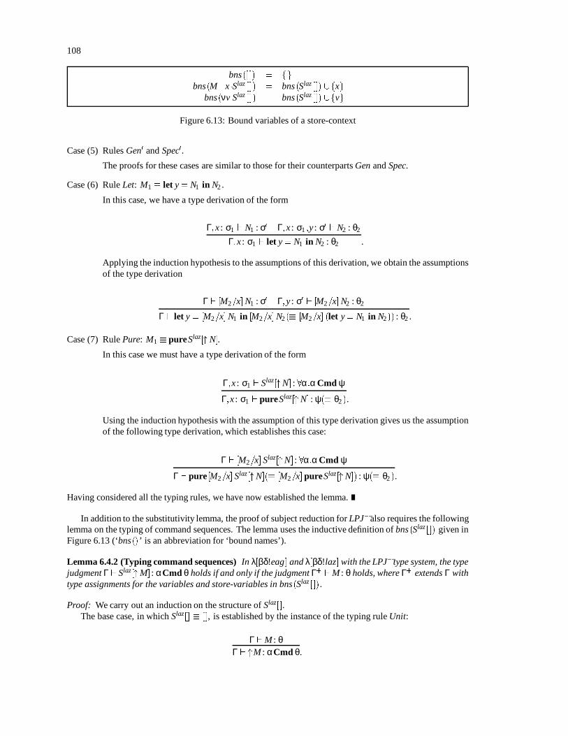
108

bns([ ]) = fg

bns(M. x Slaz []) = bns(Slaz []) [fxgbns(νv:Slaz []) = bns(Slaz []) [fvg

Figure 6.13: Bound variables of a store-context

Case (5) Rules Gen0 and Spec0.

The proofs for these cases are similar to those for their counterparts Gen and Spec.

Case (6) Rule Let: M1 let y = N1 in N2 .

In this case, we have a type derivation of the form

Γ;x : σ1 ` N1 : σ0 Γ;x : σ1 ;y : σ0 ` N2 : θ2

Γ;x : σ1 ` let y = N1 in N2 : θ2 .

Applying the induction hypothesis to the assumptions of this derivation, we obtain the assumptionsof the type derivation

Γ ` [M2=x]N1 : σ0 Γ;y : σ0 ` [M2=x]N2 : θ2

Γ ` let y = [M2=x]N1 in [M2=x]N2( [M2=x] (let y = N1 in N2)) : θ2 .

Case (7) Rule Pure: M1 pureSlaz["N].

In this case we must have a type derivation of the form

Γ;x : σ1 ` Slaz["N] : 8α:α Cmd ψ

Γ;x : σ1 ` pureSlaz["N] : ψ( θ2 ).

Using the induction hypothesis with the assumption of this type derivation gives us the assumptionof the following type derivation, which establishes this case:

Γ ` [M2=x] Slaz["N] : 8α:α Cmd ψ

Γ ` pure[M2=x] Slaz["N]( [M2=x] pureSlaz["N]) : ψ( θ2 ).

Having considered all the typing rules, we have now established the lemma.

In addition to the substitutivity lemma, the proof of subject reduction for LPJalso requires the followinglemma on the typing of command sequences. The lemma uses the inductive definition of bns(Slaz []) given inFigure 6.13 (‘bns()’ is an abbreviation for ‘bound names’).

Lemma 6.4.2 (Typing command sequences) In λ[βδ!eag] and λ[βδ!laz] with the LPJtype system, the typejudgment Γ ` Slaz["M] : αCmd θ holds if and only if the judgment Γ+ `M : θ holds, where Γ+ extends Γ withtype assignments for the variables and store-variables in bns(Slaz []).

Proof: We carry out an induction on the structure of Slaz[].The base case, in which Slaz[] [], is established by the instance of the typing rule Unit:

Γ `M : θΓ ` "M : αCmd θ.

109

That this inference also works in the reverse direction is implied by the fact that this is the only typing rulethat infers a non-schematic type for a term of the form "M.

We now treat the two inductive cases. If Slaz[] M1 .x Slaz1 [], the relevant type inference is an instance

of the rule Seq:

Γ `M1 : αCmd θ1 Γ;x : θ1 ` Slaz1 ["M] : αCmd θ

Γ `M1 .x Slaz1 [] : αCmd θ .

If we are given the right-hand assumption of this inference by means of the induction hypothesis, the conclu-sion line follows and establishes the “if” direction of the lemma in this case, since the type environment Γ isaugmented by a type assignment for the variable x that is added when going from bns(Slaz

1 []) to bns(Slaz []) .Conversely, if we are given the conclusion line, the fact that we have only one typing rule for terms of thegiven form implies the existence of derivations for the assumptions. Applying the induction hypothesis to theright-hand assumption gives Γ1 `M : θ, where Γ1 extends Γ;x : θ1 with type assignments for all the names inbns(Slaz

1 []). But this last statement is equivalent to saying that Γ1 extends Γ with type assignments for all thenames in M1 .x Slaz

1 [], which is what we have to show.The induction case in which Slaz[] νv:Slaz

1 [] follows by similar reasoning modulo use of the inferencerule New instead of Seq.

We now state and prove the subject reduction property for LPJ.

Lemma 6.4.3 (Subject reduction) In λ[βδ!eag] and λ[βδ!laz] under the type system LPJ, if Γ `M : θ andM!N, then Γ ` N : θ.

Proof: Before we get to the heart of the proof, there are a couple of reasoning principles to note in preparation.First, it is sufficient to consider only the cases in which M is a redex. We note that (1) every subtree of a

valid type derivation is a valid type derivation and (2) the typing rule for each syntactic construct depends ona type judgment for each of that construct’s subterms. Thus if we are given a valid type derivation for a termcontaining a deeply embedded redex, there will exist some subtree of that type derivation that establishes atype for the redex.

Second, we need to account for the interaction of the generalization and specialization rules with our prooftechnique. For each redex, we start with the hypothesis that there exists a valid type derivation for that redex.We then observe that the syntax-directed typing rule for the root syntactic construct of the redex requires thatcertain judgments concerning subterms of the redex must be valid; finally, we use these judgments to constructa valid type derivation for the reduct.

It is possible, however, that there may be more than one valid type derivation for the term in question, sincethe rules Spec and Gen relate judgments concerning the same term in the premise and conclusion. There maythus be some intervening applications of these polymorphism-related rules between the root of the derivationtree and the first application of the syntactically required typing rule. Nonetheless, it should be clear frominspection of the typing rules that every type derivation for a term must contain a unique instance of a syntax-directed typing that is closest to the root of the derivation. It is to this closest syntax-directed rule applicationthat we are referring in the rest of the proof when we say that a type derivation must have a certain form.Furthermore, since specializations and generalizations only depend on the type environment and adjudgedtype (and not on the typed term) it is possible to reapply them after proving that a redex and its reduct havethe same type. This reasoning lets us complete the round trip from the original type derivation for the redex tothe trimmed type derivation with a syntax-directed rule at the root to a trimmed type derivation for the reductand finally back to a full derivation for the reduct having the original type.

We consider one case for each reduction rule in λ[βδ!eag] and λ[βδ!laz].

Case (1) Rule β: (λx:M1)M2 ! [M2=x]M1.

A β-redex must have a type derivation of the form

110

Γ;x : θ1 `M1 : θ2

Γ ` λx:M1 : θ1 ! θ2 Γ `M2 : θ1

Γ ` (λx:M1)M2 : θ2 .

The assumptions we are forced to make if we assume the existence of this type derivation are ex-actly the hypotheses of the substitution lemma (Lemma 6.4.1), which allows us to conclude thatΓ ` [M2=x]M1 : θ2 , which is the required judgment concerning the type of the reduct.

Case (2) Rule δ.

This case is covered by our assumptions concerning the types of primitives defined in the calculus.

Case (3) Rule assoc: (M1 .x2 M2).x3 M3 ! M1 .x2 M2 .x3 M3 .

A type derivation for an assoc-redex must have the form

Γ `M1 : αCmd θ1 Γ;x2 : θ1 `M2 : αCmd θ2

Γ `M1 .x2 M2 : αCmd θ2 Γ;x3 : θ2 `M3 : αCmd θ3

Γ `M1 .x2 M2 .x3 M3 : αCmd θ3 .

The judgment Γ;x3 : θ2 `M3 : αCmd θ3 can be weakened to Γ;x2 : θ1 ;x3 : θ2 ` M3 : αCmd θ3 ; thevariable x2 cannot occur free in M3 because M3 is outside the scope of x2 in the redex, and we observeBarendregt’s convention that bound and free variables have distinct names. We can thus use theassumptions of the type derivation above to establish the following type derivation for the reduct:

Γ `M1 : αCmd θ1

Γ;x2 : θ1 `M2 : αCmd θ2 Γ;x2 : θ1 ;x3 : θ2 `M3 : αCmd θ3

Γ;x2 : θ1 `M2 .x3 M3 : αCmd θ3

Γ `M1 .x2 M2 .x3 M3 : αCmd θ3 .

Case (4) Rule unit: "M1 .x M2 ! [M1=x]M2.

A type derivation for the redex has the form

Γ `M1 : θ1 (α 62 fv θ1 ;α 62 fv Γ )

Γ ` "M1 : αCmd θ1 Γ;x : θ1 `M2 : αCmd θ2

Γ ` "M1 .x M2 : αCmd θ2 .

The assumptions of this type derivation match the hypotheses of Lemma 6.4.1, so we can infer thejudgment Γ ` [M1=x]M2 : αCmd θ2 for the reduct, which is what is required.

Case (5) Rule extend: (νv:M1).x M2 ! νv:M1 .x M2 .

A valid type derivation for an extend-redex takes the form

Γ;v : αRef θ0 `M1 : αCmd θ1

Γ ` νv:M1 : αCmd θ1 Γ;x : θ1 `M2 : αCmd θ2

Γ ` (νv:M1).x M2 : αCmd θ2 .

The assumptions of this type derivation (modulo some weakening to make them fit the inferencerules) give us the assumptions of the following type derivation for the reduct:

Γ;v : αRef θ0 `M1 : αCmd θ1 Γ;v : αRef θ0 ;x : θ1 `M2 : αCmd θ2

Γ;v : αRef θ0 `M1 .x M2 : αCmd θ2

Γ ` νv:M1 .x M2 : αCmd θ2 .

111

Case (6) Rule assign-result: v :=M1 .x M2 ; x 2 fv M2.

A valid type derivation for the redex in this case takes the form

Γ ` v :=M1 : αCmd () Γ;x : () `M2 : αCmd θ2

Γ ` v :=M1 .x M2 : αCmd θ2 .

Taking into account the global type assignment () : () and the assumption Γ;x : () `M2 : αCmd θ2 ,the substitution lemma lets us conclude Γ ` [( )=x]M2 : αCmd θ2 . We use this judgment aong withthe other assumption to construct the following valid type derivation for the reduct:

Γ ` v :=M1 : αCmd () Γ;z : () ` [( )=x]M2 : αCmd θ2

Γ ` v :=M1; [( )=x]M2 : αCmd θ2 ,

where z is a variable resulting from the expansion of the abbreviation “;”, and we have weakenedthe judgment given to us by the substitution lemma.

Case (7) Rule fuse: v :=M1; v? .x M2 ! v :=M1; [M1=x]M2.

A type derivation for the redex takes the form

Γ ` v : αRef θ0 Γ `M1 : θ0

Γ ` v :=M1 : αCmd ()

Γ;z : () ` v : αRef θ0

Γ;z : () ` v? : αCmd θ0 Γ; z : ();x : θ0 `M2 : αCmd θ2

Γ;z : () ` v? .x M2 : αCmd θ2

Γ ` v :=M1; v? .x M2 : αCmd θ2 ,

where the variable z arises from the expansion of the syntactic abbreviation “;” and occurs nowhereexcept its binding occurrence.

With a suitable weakening of the assumptions given by the above type derivation we can establish atype derivation for the reduct in two steps. First, the assumptions Γ;z : () `M1 : θ0 (note the weak-ened type judgment) and Γ;z : ();x : θ0 `M2 : αCmd θ2 match the hypotheses of Lemma 6.4.1, sowe can infer Γ;z : () ` [M1=x]M2 : αCmd θ2 . Second and finally, we now have enough assumptionsto construct the following type deriva for the reduct:

Γ ` v :=M1 : αCmd () Γ;z : () ` [M1=x]M2 : αCmd θ2

Γ ` v :=M1; [M1=x]M2 : αCmd θ2 .

Case (8) Rule bubble-assign: v :=M1; w?.x M2 ! w?.x v := M1; M2

A type derivation for this form of redex takes the form

Γ ` v : αRef θ0 Γ `M1 : θ0

Γ ` v :=M1 : αCmd ()

Γ; z : () ` w : αRef θ1

Γ; z : () ` w?: αCmd θ1 Γ; z : ();x : θ1 `M2 : αCmd θ2

Γ; z : () ` w?.x M2 : αCmd θ2

Γ ` v :=M1; w?.x M2 : αCmd θ2 .

The assumptions of the above derivation allow us to establish the following type derivation for thereduct. We can legitimately drop type assignments concerning the variable z from the type environ-ment because it occurs nowhere except its bindingoccurrence; we also weaken some type judgmentsto match the type inference rules:

112

Γ ` w : αRef θ1

Γ ` w?: αCmd θ1

Γ;x : θ1 ` v : αRef θ0 Γ;x : θ1 `M1 : θ0

Γ;x : θ1 ` v :=M1 : αCmd () Γ;z : ();x : θ1 `M2 : αCmd θ2

Γ;x : θ1 ` v :=M1; M2 : αCmd θ2

Γ ` w?.x v := M1; M2 : αCmd θ2 .

Case (9) Rule bubble-new: νv:w? .x M ! w?.x νv:M .

Type derivations for this form of redex take the form

Γ;v : αRef θ0 ` w : αRef θ1

Γ;v : αRef θ0 ` w?: αCmd θ1 Γ;v : αRef θ0 ;x : θ1 `M : αCmd θ2

Γ;v : αRef θ0 ` w?.x M : αCmd θ2

Γ ` νv:w? .x M : αCmd θ2 .

Before we use the assumptions of this type derivation to derive the same type for the reduct, we mustobserve that the judgment Γ;v : αRef θ0 `w : αRef θ1 actually implies the judgment Γ`w : αRef θ1 :since v and w are distinct store-variables when this reduction rule applies, the first judgment couldonly hold if Γ already holds a type assignment for w. We can now proceed in the usual way:

Γ ` w : αRef θ1

Γ ` w?: αCmd θ1

Γ;x : θ1 ;v : αRef θ0 `M : αCmd θ2

Γ;x : θ1 ` νv:M : αCmd θ2

Γ ` w?.x νv:M : αCmd θ2 .

Case (10) Rule pure-eager: pureSeag[" (λx:M)] ! λx:pure Seag["M].

A type derivation for such a redex must have the form

Γ ` Seag[" (λx:M)] : αCmd (θ!ψ)(α 62 fv Γ)

Γ ` Seag[" (λx:M)] : 8α:α Cmd (θ! ψ)

Γ ` pureSeag[" (λx:M)] : θ! ψ .

Using the assumption of this type derivation, Lemma 6.4.2 tells us that the judgment

Γ+ ` λx:M : θ! ψ

holds for some type environment Γ+ that extends Γ with type assignments for all the names in bns(Seag []).Lemma 6.4.2 applies because every eager store-context Seag[] is also a lazy store-context. This judg-ment, in turn, must arise from an application of the typing rule Abs under the assumption Γ+ ;x : θ `M : ψ. With this judgment in hand, we reverse the direction of reasoning (noting that the type envi-ronment Γ+ ;x : θ can also be thought of as being an extension (Γ;x : θ)+ of Γ;x : θ with type assign-ments for all the names in bns(Seag []). In this way we obtain the following type derivation for thereduct:

(Γ;x : θ)+ `M : ψ(Lemma 6.4.2)

Γ;x : θ ` Seag["M] : αCmd ψ(α 62 fv Γ;x : θ)

Γ;x : θ ` Seag["M] : 8α:α Cmd ψ

Γ;x : θ ` pureSeag["M] : ψΓ ` λx:pure Seag["M] : θ! ψ .

The cases of the other two forms of pure-eager-redex are proved similarly.

113

Λok ::= v j f j λx:M j cn M1 Mk; (k n) j v? .x M j Θok

Θok ::= v? j v :=Λok j "Λok j νv:v := M; Θok j v :=M; Θok

Figure 6.14: The language Λok of non-stuck normal forms

Case (11) Rule pure-lazy: pureSlaz[" (λx:M)] ! λx:pure Slaz["M].

The proof of this case is identical to that for the pure-eager.

Case (12) Rule let: let x = M1 in M2 ! [M1=x]M2.

In this case, a type derivation must take the form

Γ `M1 : σ Γ;x : σ `M2 : θΓ ` let x = M1 in M2 : θ .

By Lemma 6.4.1, the assumptions of this derivationsuffice to establish the judgment Γ` [M1=x]M2 : θ,which is the typing we desire for the reduct.

Since we have established the property of subject reduction for each of the possible forms of redex in LPJ,Lemma 6.4.3 is now proved.

We now face the task of proving that the type system LPJ is safe for the calculi λ[βδ!eag] and λ[βδ!laz].In order to state this result precisely we formalize the requirements for type safety stated in Section 6.2. Asdiscussed in that section, the primary responsibility of the type system is to ensure that certain stuck terms(normal forms that are not answer terms) cannot arise among the well-typed terms. If we can show this, thenwe can deduce that no computation starting from a well-typed term can go wrong: Lemma 6.4.3 assures thatsubsequent reducts of such a term retain the same type, and thus no stuck term can ever arise.

Our proof is that of [Chen and Odersky, 1994], adapted slightly to make use of LPJ. This proof proceedsby giving an inductively-defined language of non-stuck normal forms and proving that all the well-typed nor-mal forms belong to this language. Figure 6.14 gives this language of non-stuck normal forms. The formνv:v := M; Θok accounts for our convention that all store-variables are initialized immediately after being de-clared.

Lemma 6.4.4 (Well-typed normal forms) In λ[βδ!eag] and λ[βδ!laz]with the LPJ type system, if Γ`M : θ,where Γ fv1 : α1 Ref θ1 ;: : : ;vm : αm Ref θmg and M is irreducible, then M 2 Λok.

Proof: We prove the lemma by induction on the structure the term M in the statement of the lemma. Weconsider every possible syntactic construction of M and show that each is either reducible (and hence not asubject of the lemma) or is in Λok .

Case (1) M f , M cn, or M λx:M1 .

In all these cases the definition of Λok gives M 2 Λok directly.

Case (2) M M1 M2.

We consider several cases based on the syntactic form of M1. By the inductionhypothesis, M1 2Λok .Furthermore, since M1 is well-typed and occurs applied to another term within the well-typed typedM, it must be assigned a functional type. Among the elements of Λok only those of the followingforms satisfy this requirement:

(a) M1 f .Since we are assuming that primitives are typed as functions taking arguments of constructedtype or function type, the argument term M2 must have a constructed type or function type. Fur-thermore, the induction hypothesis demands that M2 2 Λok . Thus the only forms M2 can takein this case are f, λy:M0

2, or cn M21 M2k

; (k n). All these possibilities make M intoa δ-redex (since we assume that primitives are total on their domains of definition). Since thisform for M is not irreducible, it is removed from consideration.

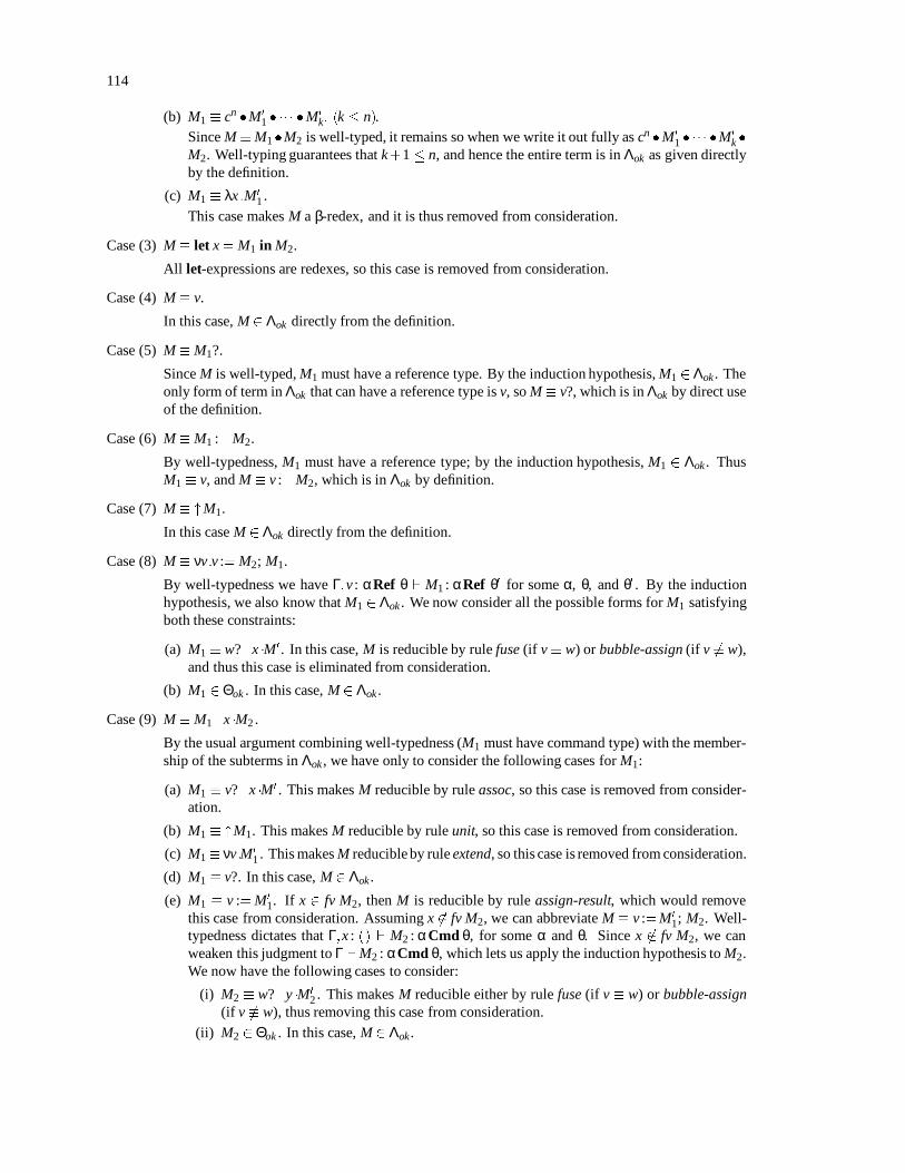
114

(b) M1 cn M0

1 M0

k; (k n).Since MM1 M2 is well-typed, it remains so when we write it out fully as cn M0

1 M0

k

M2. Well-typing guarantees that k+1 n, and hence the entire term is in Λok as given directlyby the definition.

(c) M1 λx:M0

1 .This case makes M a β-redex, and it is thus removed from consideration.

Case (3) M let x = M1 in M2.

All let-expressions are redexes, so this case is removed from consideration.

Case (4) M v.

In this case, M 2 Λok directly from the definition.

Case (5) M M1?.

Since M is well-typed, M1 must have a reference type. By the induction hypothesis, M1 2Λok . Theonly form of term in Λok that can have a reference type is v, so M v?, which is in Λok by direct useof the definition.

Case (6) M M1 :=M2.

By well-typedness, M1 must have a reference type; by the induction hypothesis, M1 2 Λok . ThusM1 v, and M v :=M2, which is in Λok by definition.

Case (7) M "M1.

In this case M 2 Λok directly from the definition.

Case (8) M νv:v := M2; M1.

By well-typedness we have Γ;v : αRef θ ` M1 : αRef θ0 for some α, θ, and θ0 . By the inductionhypothesis, we also know that M1 2 Λok . We now consider all the possible forms for M1 satisfyingboth these constraints:

(a) M1 w?.x M0 . In this case, M is reducible by rule fuse (if v w) or bubble-assign (if v 6 w),and thus this case is eliminated from consideration.

(b) M1 2Θok . In this case, M 2 Λok .

Case (9) M M1 .x M2 .

By the usual argument combining well-typedness (M1 must have command type) with the member-ship of the subterms in Λok , we have only to consider the following cases for M1:

(a) M1 v?.x M0 . This makes M reducible by rule assoc, so this case is removed from consider-ation.

(b) M1 "M1. This makes M reducible by rule unit, so this case is removed from consideration.

(c) M1 νv:M0

1 . This makes M reducible by rule extend, so this case is removed from consideration.

(d) M1 v?. In this case, M 2 Λok .

(e) M1 v := M0

1. If x 2 fv M2, then M is reducible by rule assign-result, which would removethis case from consideration. Assuming x 62 fv M2, we can abbreviate M v :=M0

1; M2. Well-typedness dictates that Γ;x : () ` M2 : αCmd θ, for some α and θ. Since x 62 fv M2, we canweaken this judgment to Γ `M2 : αCmd θ, which lets us apply the induction hypothesis to M2.We now have the following cases to consider:

(i) M2 w? .y M0

2 . This makes M reducible either by rule fuse (if v w) or bubble-assign(if v 6 w), thus removing this case from consideration.

(ii) M2 2Θok . In this case, M 2 Λok .

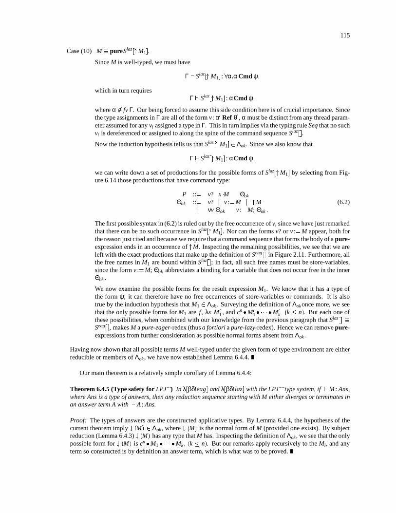
115

Case (10) M pureSlaz["M1].

Since M is well-typed, we must have

Γ ` Slaz["M1] : 8α:α Cmd ψ;

which in turn requiresΓ ` Slaz["M1] : αCmd ψ;

where α 62 fv Γ. Our being forced to assume this side condition here is of crucial importance. Sincethe type assignments in Γ are all of the form v : α0 Ref θ0 , α must be distinct from any thread param-eter assumed for any vi assigned a type in Γ. This in turn implies via the typing rule Seq that no suchvi is dereferenced or assigned to along the spine of the command sequence Slaz[].

Now the induction hypothesis tells us that Slaz["M1]2 Λok . Since we also know that

Γ ` Slaz["M1] : αCmd ψ;

we can write down a set of productions for the possible forms of Slaz["M1] by selecting from Fig-ure 6.14 those productions that have command type:

P ::= v? .x M j Θok

Θok ::= v? j v :=M j "Mj νv:Θok j v :=M; Θok :

(6.2)

The first possible syntax in (6.2) is ruled out by the free occurrence of v, since we have just remarkedthat there can be no such occurrence in Slaz["M1]. Nor can the forms v? or v :=M appear, both forthe reason just cited and because we require that a command sequence that forms the body of a pure-expression ends in an occurrence of "M. Inspecting the remaining possibilities, we see that we areleft with the exact productions that make up the definition of Seag[] in Figure 2.11. Furthermore, allthe free names in M1 are bound within Slaz[]; in fact, all such free names must be store-variables,since the form v :=M; Θok abbreviates a binding for a variable that does not occur free in the innerΘok .

We now examine the possible forms for the result expression M1. We know that it has a type ofthe form ψ; it can therefore have no free occurrences of store-variables or commands. It is alsotrue by the induction hypothesis that M1 2 Λok . Surveying the definition of Λokonce more, we seethat the only possible forms for M1 are f , λx:M0

1 , and cn M0

1 M0

k; (k n). But each one ofthese possibilities, when combined with our knowledge from the previous paragraph that Slaz[] Seag[], makes M a pure-eager-redex (thus a fortiori a pure-lazy-redex). Hence we can remove pure-expressions from further consideration as possible normal forms absent from Λok .

Having now shown that all possible terms M well-typed under the given form of type environment are eitherreducible or members of Λok , we have now established Lemma 6.4.4.

Our main theorem is a relatively simple corollary of Lemma 6.4.4:

Theorem 6.4.5 (Type safety for LPJ) In λ[βδ!eag] and λ[βδ!laz] with the LPJ type system, if `M : Ans,where Ans is a type of answers, then any reduction sequence starting with M either diverges or terminates inan answer term A with ` A : Ans.

Proof: The types of answers are the constructed applicative types. By Lemma 6.4.4, the hypotheses of thecurrent theorem imply # (M) 2 Λok , where # (M) is the normal form of M (provided one exists). By subjectreduction (Lemma 6.4.3) # (M) has any type that M has. Inspecting the definition of Λok , we see that the onlypossible form for # (M) is cn M1 Mk; (k n). But our remarks apply recursively to the Mi, and anyterm so constructed is by definition an answer term, which is what was to be proved.

116

6.5 The prospect for an untyped version of LPJThe success of the central technique of LPJ in underpinning the LPJ type system for λ[βδ!eag] and λ[βδ!laz]suggests that we investigate whether the unrestricted LPJ type system might play a similar role with respect tosome untyped lambda-calculus with assignments. As we have already remarked, LPJ is unsafe for λ[βδ!eag]and λ[βδ!laz] themselves. For example, the term

pureνv:v := 1; (pure "v)?.x " x (6.3)

is typable in LPJ but gets stuck in λ[βδ!eag] owing to the attempt to return a store-variable from the innerpure.

As a first attempt, we might consider lifting the restriction on the forms of term that can be returned frompure constructs. This, however, leads to immediate disaster, because store-contexts can bind variables thatmight be present in the returned form. We already know that imposing a condition that no variables be freedby purification leads to the problem that brings down the ILC and Chen/Odersky type systems, so we mustclassify this approach as unpromising.

The next attempt (one to which this author has devoted considerable energy) is to introduce into the un-typed calculus a new kind of name for tagging threads, in the hope that some sort of run-time check for threadidentity might cause bad purification attempts to get stuck. Unfortunately, it is not enough that all such at-tempts get stuck: our desire for confluence demands that all stuck terms resulting from reduction starting atthe same term should be identical. This demand is difficult to satisfy: a characteristic failure is that pure-contexts become duplicated around a portion of the result on one reduction path but not on another. Somesort of idempotence rule for pure-contexts seems in order, but at this point the calculus becomes vastly over-balanced toward technicalities—the hope that an untyped calculus might expose computational intuitions islost.

These negative experiences lead to the tentative conclusion that in order to obtain the generality of purifi-cation afforded by the Launchbury/Peyton Jones type system it may be best just to work in a typed frameworkfrom the start.

6.6 Chapter summaryIn this chapter, we have investigated the construction of a safe type system for λ[βδ!eag] and λ[βδ!laz]. Wehave noted a known flaw in the previous efforts along these lines (Chen/Odersky and ILC), and have con-structed and proved safe a hybrid (LPJ) of the flawed approaches with the type system proposed by Launch-bury and Peyton Jones.

7In conclusion

We now conclude this study of lambda-calculi with assignment. Section 7.1 acknowledges the ways in whichthe actual work falls short of covering its entire scope; Section 7.2 looks beyond the boundaries we have set forthis dissertation to see what further work might take advantage of the foundations we have established here.Section 7.3 provides a final summary of the work we have presented.

7.1 Unfinished businessThis dissertation has one major hole: our failed attempt to incorporate the lazy-store calculus λ[βδ!laz] intothe scheme of the conservative-extension results presented in Section 5.2. As we noted in Section 5.2.6, theprospects for such a proof using techniques analogous to those employed for λ[βδ!eag] are rather dim, sincethe syntactic structure required for a continuation-passing-style encoding of the command execution order forλ[βδ!laz] is directly at odds with the nesting structure required for the local-name construct νw:M. It might bepossible to use Odersky’s de Bruijn-like encoding scheme from [Odersky, 1993b] directly, but this approachlacks the satisfying aspect of dealing with commands and name-locality in a modular fashion. Progress infilling this gap seems to require new insight which the author of this dissertation has not yet achieved.

7.2 Future WorkThe calculi introduced in this dissertation only model store-variables with a single assignable data component,and only describe conventional sequential control constructs that can be modeled by basic blocks or procedureinvocations. We now indicate briefly two directions in which our core treatment may be extended with somefurther effort. In Section 7.2.1, we consider compound mutable entities (such as data structures or arrays) thatare allocated all at once, but have independently assignable parts. In Section 7.2.2 we consider the extensionof the techniques used in this dissertation to model non-local control constructs such as Scheme’s call=cc .

7.2.1 Mutable arrays and data structures

Our entire treatment of mutable data in this dissertation has been in terms of store-variables which can be asso-ciated with a single data value. As previously remarked on page 18, this treatment does not exactly correspondto the notion of data structure present in conventional programming languages such as C. In this section wesketch some possible further work toward bridging this semantic gap.

Object identity versus component identity

The notion of store-variable treated in this dissertation resembles the notion of variable in conventional imper-ative programming languages, but the two concepts are far from identical. Data structures in C are identifiedwith the storage they occupy. This means, for example, that in a structure with two integer fields the addressof the whole structure and of the first field are the same, and that programs can detect this sharing by assigningto the whole structure and the components separately. With store-variables, on the other hand, every allocatedentity has a distinct identity. If we want to have a structure containing two mutable integer fields, yet also itselfmutable, we are forced to allocate a single store-variable containing an immutable pair of two store-variablescontaining integers. To satisfy the semantics of the functional language, the implementation would have tobe something like a pointer to a structure of two (pointers to) integers. A conventional language implementa-tion, however, would identify the storage allocated to the structure with the storage allocated to the containedreferences. Although the difference is not semantically detectable in our functional calculi with assignment,the additional storage allocation would surely be visible to performance tools in any practical software devel-opment environment.

What is lacking in our calculi is the ability to subdivide the mutability of a store-variable. A reasonablesolution would be to introduce some structure on store-variable names so that a cluster of names can itself be

117

118

given a unique name. The semantics could be defined by translation into the calculus with individual store-variables, taking into account type information to guide the identification of storage for contained referenceswith storage for the container reference.

Arrays and pointer arithmetic

At first glance there seems to be no problem in adding the conventional notion of data arrays to our languages.If we add our assignable variables to a functional programming language already having immutable arrays,we can simulate a conventional mutable array by an immutable array of store-variables. However, in lightof the issue raised immediately above, we can see that more is required if the array itself is to be a mutableobject. Extending the solution suggested for structures above, we could introduce a notion of store-variablenames qualified with indices rather than component names.

7.2.2 Advanced control constructs

It is possible to augment the calculus λ[βδ!eag] with a non-local control operator in the style of [Felleisenet al., 1987; Felleisen and Hieb, 1992; Felleisen, 1988]. This operator is defined in a way that works with anysyntactic monad; however, we will only consider it in the context of our calculi of assignments.

The cited works by Felleisen and his colleagues investigate the introduction of syntactically-defined con-trol operators into call-by-value lambda-calculi for the purpose of providing an operational semantics for thelanguage Scheme [Clinger and Rees, 1991] including the construct call/cc. Our aim here differs from theirsin several respects. First, our base lambda-calculus is call-by-name rather than call-by-value. Second, wedo not incorporate our control construct into the applicative language; rather, we have it operate on a syntac-tically distinct monadic fragment of our calculus. We could thus conjecture that an extension of functionalprogramming with control constructs based on our monad-inspired approach might actually be a conservativeextension of the base language, whereas this is not expected of a model of Scheme. Although we are not ina position to deny that a calculus modeling Scheme with call/cc can be a conservative extension of the call-by-value lambda-calculus, this is a reasonable conjecture because of the ability of a term containing call/ccto grab its evaluation context. Perhaps such a term can discover differences in evaluation patterns betweenterms that are operationally equivalent in the base calculus. 1 At any rate, we are motivated to study controloperators by the methods of this dissertation.

A control operator for the command calculi

The idea behind the control operator C is simple. If a procedure is in!. -normal form, every tail of the proce-dure (portion following a .) represents the future of the computation (the continuation) from that point. Thecontrol operator should be able to substitute a different continuation while storing the old one.

Formally, the action of the control operator is defined by Figure 7.1, which gives the rule implementing thereplacement-with-remembrance of the current continuation. The control operator takes a procedure, called theescape continuation as an argument, and produces an escape procedure. At the point where the escape proce-dure is invoked, the then-current continuation is captured and passed as argument to the escape continuation,which is where execution now continues.

The usual control operators call=cc and abort can be defined in terms of C as follows:

call=cc λm:C (λk:m (λx:C (λk0 :k x)).x k x)abort λx:C (λk:" x)

1It is also strongly suggestive that [Felleisen, 1991] finds that an idealized Scheme with call/cc is more expressive than pure Schemein a well-defined sense that is related to operational semantics.

119

pureSlaz[(C M).x N ] ! pureSlaz[M (λx:N)]

Figure 7.1: Rule for control operator

Interaction of control and assignment

It is interesting to note that the introduction of the operator C is incompatible with λ[βδ!laz]. Consider theterm

pureC (λy:" 2).x " 1:

We can reduce this by a pure-lazy-reduction to 1, or via a control reduction to

pure(λy:" 2) (λx:" 1);

which reduces to 2 by β followed by pure-lazy. The lazy-store calculus with the added control operator is thusnot Church-Rosser. This counterexample does not apply in λ[βδ!eag] because the purification contexts theredo not allow control operators to remain along the spine of the command sequence. This failure of a coun-terexample is not the same thing as having a proof of Church-Rosser for λ[βδ!eag] plus the control operator,so it would be interesting further work to work out the theory of this calculus, compare it with the work ofFelleisen and colleagues cited above, and find the deep reason why the simple approach fails in the lazy-storecalculus.

This concludes our discussion of possible future work based on the work in this dissertation.

7.3 Summary of technical resultsWe have introduced and studied formal representations of two potential paradigms of functional programmingwith assignment statements. We have brought the apparatus of the study of the untyped lambda-calculus tobear on these representations, and have found that they have the Church-Rosser and standardization proper-ties just as do the foundations of pure functional programming. We have explored the operational-equivalencetheory implied by this reduction-semantics basis and have found it to correspond to our informal understand-ing in some simple test cases. The proposed calculi correspond in a precise way with store-computations asmodeled by alternative calculi which represent the store explicitly, and both calculi are conservative exten-sions of appropriately chosen pure functional calculi. Finally, we have shown that a reasonably simple typesystem guarantees safe usage of the assignment constructs in our untyped calculi.

We hope that the theoretical results presented here will lead to the confident adoption of a safe and rea-sonable design for a programming language combining the powerful higher-order program-construction fa-cilities of functional programming with the convenient resource-consumption model of programming withassignments.

AProofs of the fundamental properties for λ[βδσeag] and λ[βδσlaz]

We give in this appendix the proofs of the Church-Rosser and standardization theorems for the calculi λ[βδσeag]and λ[βδσlaz] introduced in Chapter 5. We use the structure of the corresponding proofs in Chapter 3 as aguide in structuring the proofs in this appendix. Our presentation here is thus rather sketchy: we give only thefeatures that differ from those in the corresponding proofs and assume that these differing features are to beembedded in a matrix of general argument that is lifted directly from Chapter 3.

In general, the proofs for λ[βδσeag] and λ[βδσlaz] require less work than the corresponding proofs forλ[βδ!eag] and λ[βδ!laz]. The shift of the axiomatization of the store from rewriting of command-sequencesto the use of an explicit store removes many critical overlaps between rules. It is still necessary, however, tocarry out the proofs in terms of .

=-equivalence classes, since the issue that led to their introduction derivesentirely from the structure of the rules assoc and extend, which are retained in the explicit-store calculi.

A.1 The reductions!. and!!

The reduction!. is the exact same for λ[βδσeag] and λ[βδσlaz] as for λ[βδ!eag] and λ[βδ!laz], and the def-inition of!! from! and!. is derived in the same way as it is in Section 3.3.2.

The first result we establish is the analogue of Proposition 3.4.1:

Proposition A.1.1 (Commutation of association) Suppose we have M!! N via reduction of a marked redex∆, and suppose also that M!. M0: Then there exist terms M00 and N0 such that M0!.

M00, N!.N0 , and

M00!! N0 by reducing ∆00 , where ∆00 is the residual of ∆ in M00.

Proof: The statement of the proposition is illustrated by the following diagram:

M

N M0

M00

N0

!!

∆

..

..

..

..

..

..

..

..

..

.R

!.

R

@@@@@R

!.

..

..

..

..R

!.

R.

..

..

..

.

!!

..

..

..

..

∆00

:

The only critical overlap of reduction rules that survives from the proof of Proposition 3.4.1 is the overlapbetween rules unit and assoc; the old proof for this case still works here. All the other overlap cases consideredin proving Proposition 3.4.1 involve reduction rules that are no longer present in the same form in λ[βδσeag]and λ[βδσlaz].

Of the reduction rules that are introduced in the explicit-store calculi, most cannot overlap with assoc orextend because they are written in terms of the term-in-store syntax σ hMi, which is not involved in eitherof the!. -rules. The only newly-introduced rule requiring consideration is the purification rule in λ[βδσlaz],which can have!. -redexes in the store-context Slaz[]. For this case, the old proof is easily translated into the

121

122

context of λ[βδσlaz]:

z |

σ hSlaz1 [(νv:M) .x Slaz

2 [" (λy:N)]| z

]i

λy:σ hSlaz1 [(νv:M) .x Slaz

2 ["N]| z

]iz |

σ hSlaz1 [νv:M. x Slaz

2 [" (λy:N)]]i

λy:σ hSlaz1 [νv:M. x Slaz

2 ["N]]i

σpure

..

..

..

..R

extend

@@@@Rextend

..

..

..

..

.

σpure

:

With the consideration of these two rule-overlaps, we have now established Proposition A.1.1.

The reasoning by which Corollaries 3.4.2 and 3.4.3 are established is independent of the calculus to whichthey apply, so we can use this reasoning to obtain these same results for the explicit-store calculi. We havenow completed proving the necessary properties of the interaction between !. and!! for λ[βδσeag] andλ[βδσlaz].

A.2 Finite developmentsWe next prove that!! for the calculi with explicit stores has the strong finite-developments property. Thefirst step is to show that marked!! -reduction is weakly Church-Rosser on

.=-equivalence classes (analogous

to Lemma 3.5.5):

Lemma A.2.1 The weak Church-Rosser property holds for the calculi λ[βδσeag] and λ[βδσlaz]under marked!! -reduction on

.=-equivalence classes.

Proof: The cases having to do with β and δ are proved just as for the implicit-store calculi, since this core ofthe calculus is unchanged. Once again, none of the previously existing overlaps carries over, and only the newrule σpure has an overlap (with unit). The proof for this case is exactly analogous to that for the correspondingcase in Lemma 3.5.5.

The next step in proving finiteness of developments is to construct a termination measure for marked!! -reduction. The explicit-store calculi require no new reasoning here, only (1) some adjustment in the defini-tion of the weighting function W [[ ]] to reflect the new reduction rules and similarly (2) modification of Def-inition 3.5.6 to reflect the new reduction rules. We thus obtain the finiteness-of-developments property, andfurther, the stronger properties given in Theorem 3.5.12.

A.3 The Church-Rosser propertyStrong finiteness of developments gives us the Church-Rosser property exactly as in Section 3.6.

A.4 StandardizationAs in Section 3.7, the standardization theorem for the explicit-store calculi requires a lot of work concernedwith evaluation contexts and head and internal redexes. We define evaluation contexts for λ[βδσeag] andλ[βδσlaz] as given in Figures A.1 and A.2; we also augment the subterm ordering with the single new orderinggiven in Figure A.3. We reinterpret Definitions 3.7.1 and 3.7.2 in terms of these new definitions of evaluationcontext and subterm ordering.

123

E[] ::= :: : Figure 3.3 :: :j σ hE[] i

Figure A.1: Evaluation contexts for λ[βδσeag]

E[] ::= :: : Figure 3.3 :: :j σ hSlaz[E[] ]i

Figure A.2: Evaluation contexts for λ[βδσlaz]

M σ hM1i ) MM1

Figure A.3: Additional subterm ordering for λ[βδσeag] and λ[βδσlaz]

We now tackle the analogues of the lemmas concerning the preservation and separation of head and internalredexes. We first consider the analogue of Lemma 3.7.6:

Lemma A.4.1 (Heads don’t sprout) If M!i N and [N] .

=has a head redex ∆h, then [M] .

=has a head redex.

Proof: We adopt the notation used in the proof of Lemma 3.7.6, and we refer to that proof for the impor-tant discussion of the effect of the interaction of!. -reduction with the case analysis. We use the same basicdivision into three cases based on the relative positions of L0 and ∆0h.

Case (1): L0 and ∆0h are disjoint.

The argument from the proof of Lemma 3.7.6 applies with little change as far as it can be carried outindependently of the actual form of evaluation contexts. For the final part of the argument in whichwe enumerate a list of possible configurations in which ∆0 can be disjoint from ∆h, the first fourcases still apply, since they deal with forms of evaluation context that still occur in the explicit-store calculi. The only case we need to add to the list is the form E[1]σ hSlaz[" E[2]∆h ]i, where∆0 Slaz[]. In this case ∆h is an evaluation redex of M, hence there exists a head redex.

Case (2): ∆0h L0.

In this case the reasoning from the proof of Lemma 3.7.6 applies without change, since it makes nouse of the actual form of evaluation contexts.

Case (3): L0 ∆0h.

The general reasoning in this case, as well as the reasoning for the subcases for reduction rules β, δ,and unit apply without change from Lemma 3.7.6. We now treat the cases resulting from reductionrules that are introduced in λ[βδσeag] and λ[βδσlaz]. We use σ0 to denote a store that reduces toa store σ by reducing a binding for a store-variable in σ0 . Since σ0 and σ have the same domainthere is never any question of a reduction becoming available or becoming forbidden because ofthe reduction from σ0 to σ.

(a) σν: ∆h σ hνv:M1i

We construct the following table of cases:bM : eval. redex:σ h∆0i ∆0

σ hνw:C[∆0 ]i bMσ0 hνv:M1i bM

(b) σ:=: ∆h σ hv :=N1 ; M1i

We construct the following table of cases:

124

bM : eval. redex:σ h∆0i ∆0σ h∆0 :=N1 ; M1i ∆0

σ hv :=C[∆0 ]; M1i bMσ hv :=N1 ; C[∆0 ]i bMσ0 hv :=N1 ; M1i bM

(c) σ?: ∆h σ hv? .x M1i

We construct the following table of cases:bM : eval. redex:σ h∆0i ∆0σ h∆0?.x M1i ∆0

σ hv?.x C[∆0 ]i bMσ0 hv? .x M1i bM

(d) σblock : ∆h pureM1

We construct the following table of cases:bM : eval. redex:pure∆0 ∆0

pureC+ [∆0 ] bM

(e) σpeag : ∆h σ h"λx:M1i; etc.

This case applies in the calculus λ[βδσeag].

We construct the following table of cases:bM : eval. redex:σ0 h"λx:M1i bMσ h∆0i ∆0σ h"∆0i ∆0

σ h"λx:C[∆0 ]i bMThe other two forms of purifiable expression require similar arguments.

(f) σplaz : ∆h σ hSlaz["V]i; etc.

This case applies in the calculus λ[βδσlaz].

The following cases are easy to describe:

bM : eval. redex:σ0 hSlaz["V]i bMσ h∆0i ∆0σ hSlaz[∆0 ]i ∆0σ hSlaz[" ∆0]i ∆0

One of the remaining possibilities occur when ∆0 produces part of the command sequence no-tated as Slaz[]. No matter how this happens, however, bM takes the form σhSlaz

1 ["V]i, and so bMis an evaluation redex.

The last possibility is that bM σ hSlaz1 [∆0 ]i , in which case ∆0 is an evaluation redex.

We have now completed the case analysis required to establish Lemma A.4.1.

The next of the lemmas supporting the standardization theorem is the analogue of Lemma 3.7.7:

Lemma A.4.2 (Heads are preserved) Let ∆h be a head redex and ∆i be an internal redex in [M] .=

. If [M] .

=

∆i!

[N] .

=, then the residual of ∆h in #. [N] consists of a single redex that is head redex in [N] .

=.

Proof: We consider the relative positiosn of ∆h and ∆i as in the proof of Lemma 3.7.7.

125

Case (1) ∆i and ∆h are disjoint.

In this case, we reason as in the proof of Lemma 3.7.7, basing our enumeration of subcases on thecorresponding case in the proof of Lemma A.4.1 instead of Lemma 3.7.6.

Case (2) ∆i ∆h.

The reasoning used in the corresponding case in Lemma 3.7.6 applies as well in the present case—not because the argument is generic, but because the properties it requires of λ[βδ!eag] and λ[βδ!laz]are also true of λ[βδσeag] and λ[βδσlaz].

The remaining lemma supporting the proof of standardization makes a generic argument, and so it holdsfor the explicit-store calculi. We can thus prove the standardization result by the same methods as used inChapter 3.

A.5 ConclusionThe remaining work in Chapter 3, i.e. lifting results about the factored reduction relations up to the originalcalculus, can now be established by the same arguments for the explicit-store calculi.

BChanges in notation and terminology from previously publishedversions

The notation employed in this dissertation differs in several respects from that presented in the antecedentworks [Odersky et al., 1993] and [Odersky and Rabin, 1993]. There are two main reasons for the authorsdecision to change notation. First, the old notation was decidedly odd in some respects, such as in giving theassigned store-variable rightmost in an assignment command. Second, the elaboration of the mathematicalexposition in the dissertation has placed a premium on compactness of notation; thus, several keyword-stylenotations were replaced with non-alphabetic symbols. The author hopes that the exposition surrounding theintroduction of these notations compensates for the loss of familiarity.

With respect to terminology, the most troublesome point has been to decide what to call the identifiersfor assignable variables. This is a problem because the use of variable in the imperative-language culture todenote these expressions is well-entrenched, yet it conflicts with the use of variable in the lambda-calculusculture to denote an identifier for which expressions are substituted in the course of computation. We havedecided to retain the lambda-calculus usage of the simple term variable, and to consistently refer to the formerkind as store-variables. In the antecedent works we employed such terms as tag and location, but we now findtag to be too unfamiliar and location to be overly evocative of implementation issues for the level of discourseof the research presented.

There are also some differences in detail between the calculi λvar and λ[βδ!eag]. In λvar , there is only onesubstitutive rule, β, and all other rules that transmit expressions are written in terms of β. In the present work,these rules are written in terms of substitutiondirectly in order to draw a cleaner boundary between functionaland imperative rules. In retrospect, the revision does not seem to have gained much.

127

BIBLIOGRAPHY

[Amadio and Cardelli, 1991] Roberto M. Amadio and Luca Cardelli. Subtyping recursive types.In Conference Record of the Eighteenth Annual ACM Symposium onPrinciples of Programming Languages, Orlando, Florida, pages 104–118. ACM Press, January 1991.

[Ariola et al., 1995] Zena M. Ariola, Matthias Felleisen, John Maraist, Martin Odersky,and Philip Wadler. The call-by-need lambda calculus. In Proceedingsof the Twenty-second ACM Symposium on Principles of ProgrammingLanguages, San Francisco, California, pages 233–246, New York,January 1995. ACM Press.

[Barendregt, 1984] H. P. Barendregt. The Lambda Calculus: its Syntax and Semantics,volume 103 of Studies in Logic and the Foundations of Mathematics.North-Holland, Amsterdam, revised edition, 1984.

[Birtwistle et al., 1973] G.M. Birtwistle, O.-J. Dahl, B. Myhrhaug, and K. Nygaard. SIMULABegin. Auerbach, 1973.

[Chen and Odersky, 1993] Kung Chen and Martin Odersky. A type system for a lambda calculuswith assignment. Research Report YALEU/DCS/RR-963, Yale Uni-versity Department of Computer Science, May 1993.

[Chen and Odersky, 1994] Kung Chen and Martin Odersky. A type system for a lambda calcu-lus with assignments. In Masami Hagiya and John C. Mitchell, edi-tors, Theoretical Aspects of Computer Science, International Sympo-sium TACS’94, Sendai, Japan, Proceedings, pages 347–64, New York,April 1994. Springer-Verlag. Lecture Notes in Computer Science 789.

[Church, 1951] Alonzo Church. The Calculi of Lambda-Conversion, volume 6 of An-nals of Mathematics Studies. Princeton University Press, second edi-tion, 1951.

[Clinger and Rees, 1991] William Clinger and Jonathan Rees. Revised4 report on the algorith-mic language Scheme. Available via World Wide Web as http://www-swiss.ai.mit.edu/ftpdir/scheme-reports/r4rs.ps, November 1991.

[Damas and Milner, 1982] L. Damas and Robin Milner. Principal type schemes for functionalprograms. In Proceedings of the Ninth ACM Symposium on Principlesof Programming Languages, January 1982.

[Felleisen and Friedman, 1986] Matthias Felleisen and Daniel P. Friedman. Control operators, theSECD-machine, and the λ-calculus. In Martin Wirsing, editor, FormalDescriptions Of Programming Concepts III. North-Holland, 1986.

[Felleisen and Friedman, 1987a] Matthias Felleisen and Daniel P. Friedman. A calculus for assignmentsin higher-order languages. In Conference Record of the FourteenthAnnual ACM Symposium on Principles of Programming Languages.Papers Presented at the Symposium, Munich, West Germany, pages314–325, New York, January 1987. Association for Computing Ma-chinery.

[Felleisen and Friedman, 1987b] Matthias Felleisen and Daniel P. Friedman. A reduction semanticsfor imperative higher-order languages. In J. W. de Bakker, A. J. Nij-man, and P. C. Treleaven, editors, PARLE: Parallel Architectures and

129

130

Languages Europe, Volume II: Parallel Languages, Eindhoven, TheNetherlands, pages 206–223, New York, June 1987. Springer-Verlag.Lecture Notes in Computer Science 259.

[Felleisen and Hieb, 1992] Matthias Felleisen and Robert Hieb. The revised report on the syn-tactic theories of sequential control and state. Theoretical ComputerScience, 103:235–271, 1992.

[Felleisen et al., 1987] Matthias Felleisen, Daniel P. Friedman, Eugene Kohlbecker, andBruce Duba. A syntactic theory of sequential control. TheoreticalComputer Science, 52(3):205–237, 1987.

[Felleisen, 1987] Matthias Felleisen. A calculus for assignments in higher-order lan-guages. In Proceedings, Fourteenth Annual ACM Symposium on Prin-ciples of Programming Languages, pages 314–325, January 1987.

[Felleisen, 1988] Matthias Felleisen. The theory and practice of first-class prompts.In Conference Record of the Fifteenth Annual ACM Symposium onPrinciples of Programming Languages, pages 180–190. ACM, ACMPress, January 1988.

[Felleisen, 1991] Matthias Felleisen. On the expressive power of programming lan-guages. Science of Computer Programming, 17:35–75, 1991.

[Fischer, 1972] Michael J. Fischer. Lambda calculus schemata. In Proceedings ofthe ACM Conference on Proving Assertions about Programs, pages104–109, January 1972. SIGPLAN Notices, Vol.7, no. 1 and SIGACTNews, No. 14.

[Fischer, 1993] Michael J. Fischer. Lambda calculus schemata. Lisp and SymbolicComputation, 6(3/4):259–288, November 1993.

[Fradet, 1991] Pascal Fradet. Syntactic detection of single-threading using continua-tions. In John Hughes, editor, Proceedings Functional ProgrammingLanguages and Computer Architecture, 5th ACM Conference, Cam-bridge, MA, USA, pages 241–258. Springer-Verlag,August 1991. Lec-ture Notes in Computer Science 523.

[Girard et al., 1989] Jean-Yves Girard, Yves Lafont, and Paul Taylor. Proofs and Types,volume 7 of Cambridge Tracts in Theoretical Computer Science.Cambridge University Press, 1989.

[Girard, 1987] Jean-Yves Girard. Linear logic. Theoretical Computer Science, 50:1–102, 1987.

[Girard, 1990] Jean-Yves Girard. The system F of variable types, fifteen yearslater. In Gerard Huet, editor, Logical Foundations of Functional Pro-gramming, The UT Year of Programming Series, chapter 6. Addison-Wesley Publishing Company, Inc., 1990.

[Gordon, 1994] Andrew D. Gordon. Functional Programming and Input/Output. Dis-tinguished Dissertations in Computer Science. Cambridge UniversityPress, New York, 1994.

[Graham and Kock, 1991] T. C. Nicholas Graham and Gerd Kock. Domesticating imperativeconstructs so that they can live in a functional world. In J. Maluszynskiand M. Wirsing, editors, Programming Language Implementation and

131

Logic Programming, pages 51–62. Springer-Verlag, August 1991.Lecture Notes in Computer Science 528.

[Guzman and Hudak, 1990] Juan Guzman and Paul Hudak. Single-threaded polymorphic lambdacalculus. In Proceedings, Fifth Annual IEEE Symposium on Logic inComputer Science, Philadelphia, Pennsylvania, pages 333–343, LosAlamitos, California, June 1990. IEEE Computer Society Press.

[Guzman, 1993] Juan Carlos Guzman. On expressing the mutation of state in a func-tional programming language. Research Report YALEU/DCS/RR-962, Yale University, Department of Computer Science, New Haven,Connecticut, May 1993. PhD Thesis.

[Hindley, 1969] J. Roger Hindley. The principal type scheme of an object in com-binatory logic. Transactions of the American Mathematical Society,146:29–60, December 1969.

[Huang and Reddy, 1995] H. Huang and U.S. Reddy. Type reconstruction for SCI. In Proceed-ings of the Glasgow Functional Programming Workshop, New York,1995. Springer-Verlag. To appear.

[Hudak and Sundaresh, 1988] Paul Hudak and Raman S. Sundaresh. On the expressiveness of purelyfunctional I/O systems. Research Report YALEU/DCS/RR-665, YaleUniversity, Department of Computer Science, New Haven, Connecti-cut, December 1988.

[Hudak et al., 1992] Paul Hudak, Simon Peyton Jones, and Philip Wadler. Report on theprogramming language Haskell: a non-strict, purely functional lan-guage, version 1.2. Technical Report YALEU/DCS/RR-777, YaleUniversity Department of Computer Science, March 1992. Also inACM SIGPLAN Notices, Vol. 27(5), May 1992.

[Hudak, 1992] Paul Hudak. Mutable abstract datatypes. Research ReportYALEU/DCS/RR-914, Yale University Department of Computer Sci-ence, December 1992.

[Huet, 1980] Gerard Huet. Confluent reductions: Abstract properties and applica-tions to term rewriting systems. Journal of the ACM, 27(4):797–821,1980.

[Jouvelot and Gifford, 1989] Pierre Jouvelot and David K. Gifford. Reasoning about continuationswith control effects. In Proceedings of the ACM SIGPLAN Conferenceon Programming Language Design and Implementation, pages 218–226. ACM, ACM Press, June 1989.

[Klop, 1992] J.W. Klop. Term rewriting systems. In S. Abramsky, Dov M. Gab-bay, and T.S.E. Maibaum, editors, Handbook of Logic in ComputerScience, Volume 2, Background: Computational Structures, pages 1–116. Oxford University Press, Clarendon Press, New York, 1992.

[Knuth and Bendix, 1970] Donald E. Knuth and P. Bendix. Simple word problems in universalalgebras. In J. Leech, editor, Compuatational Problems in AbstractAlgebra, pages 263–297. Pergamon, Oxford, 1970.

[Lafont, 1988] Yves Lafont. The linear abstract machine. Theoretical Computer Sci-ence, 59:157–180, 1988.

132

[Landin, 1964] Peter J. Landin. The mechanical evaluation of expressions. ComputerJournal, 6(5):308–320, 1964.

[Launchbury and Peyton Jones, 1994] John Launchbury and Simon L Peyton Jones. Lazy functional statethreads. In Proceedings of the ACM SIGPLAN ’94 Conference on Pro-gramming Language Design and Implementation (PLDI), Orlando,FL, pages 24–35, New York, June 1994. ACM Press. SIGPLAN No-tices 29(6).

[Launchbury, 1993] John Launchbury. Lazy imperative programming. In SIPL ’93 ACMSIGPLAN Workshop on State in Programming Languages, Copen-hagen, Denmark, pages 46–56, June 1993.

[Lucassen and Gifford, 1988] Jon M. Lucassen and David K. Gifford. Polymorphic effect systems.In Conference Record of the Fifteenth Annual ACM Symposium onPrinciples of Programming Languages, pages 47–57. ACM, ACMPress, January 1988.

[Mason and Talcott, 1991] Ian Mason and Carolyn Talcott. Equivalence in functional languageswith side effects. Journal of Functional Programming, 1(3):287–327,July 1991.

[Mason and Talcott, 1992a] Ian A. Mason and Carolyn L. Talcott. Inferring the equivalence offunctional programs that mutate data. Theoretical Computer Science,105(2):167–215, 1992.

[Mason and Talcott, 1992b] Ian A. Mason and Carolyn L. Talcott. References, local variables,and operational reasoning. In Seventh Annual IEEE Symposium onLogic in Computer Science, Santa Cruz, California, pages 186–197,Los Alamitos, California, June 1992. IEEE Computer Society Press.

[Mason, 1986] Ian A. Mason. The Semantics of Destructive Lisp, volume 5 of CSLILecture Notes. Center for the Study of Language and Information,Ventura Hall, Stanford, CA 94305, 1986.

[Milner et al., 1990] Robin Milner, Mads Tofte, and Robert Harper. The Definition of Stan-dard ML. MIT Press, 1990.

[Milner, 1978] Robin Milner. A theory of type polymorphism in programming. Jour-nal of Computer and System Science, 17:348–375, Dec 1978.

[Milner, 1991] Robin Milner. The polyadic π-calculus: A tutorial. Report ECS-LFCS-91-180, Laboratory for Foundations of Computer Science, De-partment of Computer Science, The University of Edinburgh, October1991.

[Moggi, 1989] Eugenio Moggi. Computational lambda-calculus and monads. In Pro-ceedings, Third Annual IEEE Symposium on Logic in Computer Sci-ence. IEEE, 1989.

[Moggi, 1991] Eugenio Moggi. Notions of computation and monads. Informationand Computation, 93:55–92, 1991.

[Naur et al., 1960] Peter Naur, John W. Backus, F. L. Bauer, J. Green, C. Katz, John Mc-Carthy, Alan J. Perlis, H. Rutishauser, K. Samelson, B. Vauquois, J. H.Wegstein, A. van Wijngaarden, and M. Woodger. Report on the algo-rithmic language ALGOL 60. Communications of the ACM, 3:299–314, 1960.

133

[Naur et al., 1963] Peter Naur, J.W. Backus, F.L. Bauer, J. Green, C. Katz, J. McCarthy,A.J. Perlis, H. Rutishauser, K. Samelson, B. Vauquois, J.H. Wegstein,A. van Wijngaarden, and M. Woodger. Revised report on the algorith-mic language ALGOL 60. Communications of the ACM, 6(1):1–17,1963.

[Odersky and Rabin, 1993] Martin Odersky and Dan Rabin. The unexpurgated call-by-name, assignment, and the lambda-calculus. Research ReportYALEU/DCS/RR-930, Department of Computer Science, Yale Uni-versity, New Haven, Connecticut, May 1993.

[Odersky et al., 1992] Martin Odersky, Dan Rabin, and Paul Hudak. Call-by-name, assign-ment, and the lambda-calculus. Research Report YALEU/DCS/RR-929, Department of Computer Science, Yale University, New Haven,Connecticut, October 1992.

[Odersky et al., 1993] Martin Odersky, Dan Rabin, and Paul Hudak. Call-by-name, assign-ment, and the lambda calculus. In Proceedings of the TwentiethAnnualACM SIGPLAN-SIGACT Symposium on Principles of ProgrammingLanguages, Charleston, South Carolina, January 10–13, 1993, pages43–56, January 1993.

[Odersky, 1991] Martin Odersky. How to make destructive updates less destructive.In Conference Record of the Eighteenth Annual ACM Symposium onPrinciples of Programming Languages, Orlando, Florida, pages 25–26. ACM Press, January 1991.

[Odersky, 1993a] Martin Odersky. A syntactic method for proving observational equiv-alences. Research Report YALEU/DCS/RR-964, Department ofCompter Science, Yale University, May 1993.

[Odersky, 1993b] Martin Odersky. A syntactic theory of local names. Research ReportYALEU/DCS/RR-965, Yale University Department of Computer Sci-ence, New Haven, Connecticut, May 1993.

[Odersky, 1994] Martin Odersky. A functional theory of local names. In ConferenceRecord of POPL ’94: 21st ACM SIGPLAN-SIGACT Symposium onPrinciples of Programming Languages, Portland, Oregon, pages 48–59, New York, January 1994. ACM Press.

[O’Hearn et al., 1995] P.W. O’Hearn, A.J. Power, M. Takeyama, and R.D. Tennent. Syntacticcontrol of interference revisited. In Mathematical Foundations of Pro-gramming Semantics, pages 97–136. Elsevier, 1995. Electronic Notesin Theoretical Computer Science 1.

[Peyton Jones and Wadler, 1993] Simon L. Peyton Jones and Philip Wadler. Imperative functionalprogramming. In Conference Record of the Twentieth Annual ACMSIGPLAN-SIGACT Symposium on Principles of Programming Lan-guages, Charleston, South Carolina, January 10–13, 1993, pages 71–84. ACM Press, January 1993.

[Plotkin, 1975] Gordon D. Plotkin. Call-by-name, call-by-value, and the λ-calculus.Theoretical Computer Science, 1:125–159, 1975.

[Reddy, 1991] Uday S. Reddy. Acceptors as values: Functional programming inclassical linear logic. Available via FTP from cs.uiuc.edu, December1991.

134

[Reddy, 1993] Uday S. Reddy. A linear logic model of state. Technical report,Department of Computer Science, University of Illinois at Urbana-Champaign, January 1993. Distributed electronically.

[Reynolds, 1974] John C. Reynolds. Towards a theory of type structure. In Inter-national Programming Symposium, pages 408–425. Springer-Verlag,1974. Lecture Notes in Computer Science 19.

[Reynolds, 1978] John C. Reynolds. Syntactic control of interference. In Proceedingsof the Fifth Annual ACM Symposium on Principles of ProgrammingLanguages, pages 39–46, January 1978.

[Reynolds, 1988] John C. Reynolds. Preliminary design of the programming languageForsythe. Technical Report CMU-CS-88-159, Carnegie Mellon Uni-versity, June 1988.

[Reynolds, 1989] John C. Reynolds. Syntactic control of interference, part 2. InG. Ausiello, M. Dezani-Ciancaglini, and S. Ronchi Della Rocca, ed-itors, Automata, Languages, and Programming: 16th InternationalColloquium, Stresa, Italy, pages 704–722, New York, July 1989.Springer-Verlag. Lecture Notes in Computer Science 372.

[Riecke and Viswanathan, 1995] Jon G. Riecke and Ramesh Viswanathan. Isolating side effects in se-quential languages. In Proceedings of the Twenty-second ACM Sym-posium on Principles of Programming Languages, San Francisco,California, pages 1–12, New York, January 1995. ACM Press.

[Riecke, 1993] Jon G. Riecke. Delimiting the scope of effects. In FPCA ’93: Confer-ence on Functional Programming Languages and Computer Architec-ture, Copenhagen, Denmark, pages 146–155, New York, June 1993.ACM Press.

[Sato, 1994] Masahiko Sato. A purely functional language with encapsulated as-signment. In Masami Hagiya and John C. Mitchell, editors, Theoreti-cal Aspects of Computer Science, International Symposium TACS’94,Sendai, Japan, Proceedings, pages 179–202, New York, April 1994.Springer-Verlag. Lecture Notes in Computer Science 789.

[Schmidt, 1985] David A. Schmidt. Detecting global variables in denotational specifi-cations. ACM Transactionson Programming Languages and Systems,7(2):299–310, 1985.

[Schmidt, 1986] David A. Schmidt. Denotational Semantics: A Methodology for Lan-guage Development. Allyn and Bacon, 1986.

[Stoy, 1977] Joseph Stoy. Denotational Semantics: The Scott-Strachey Approachto Programming Language Theory. MIT Press, 1977.

[Swarup et al., 1991] Vipin Swarup, Uday S. Reddy, and Evan Ireland. Assignmentsfor applicative languages. In John Hughes, editor, Functional Pro-gramming Languages and Computer Architecture, pages 192–214.Springer-Verlag, August 1991. Lecture Notes in Computer Science523.

[Swarup, 1992] Vipin Swarup. Type Theoretic Properties of Assignments. PhD thesis,University of Illinois at Urbana-Champaign, 1992.

135

[Turner, 1985] David A. Turner. Miranda: A non-strict functional language withpolymorphic types. In Proceedings, Functional Programming Lan-guages and Computer Architecture, Nancy, France, pages 1–16.Springer-Verlag, September 1985. Lecture Notes in Computer Sci-ence 201.

[Wadler, 1990a] Philip Wadler. Comprehending monads. In Proceedings of the 1990ACM Conference on Lisp and Functional Programming, 1990.

[Wadler, 1990b] Philip Wadler. Linear types can change the world! In M. Broy andC. Jones, editors, IFIP TC 2 Working Conference on ProgrammingConcepts and Methods, Sea of Galilee, Israel, pages 347–359. NorthHolland, April 1990.

[Wadler, 1991] Philip Wadler. Is there a use for linear logic? In Proc. Symposiumon Partial Evaluation and Semantics-Based Program Manipulation,pages 255–273, June 1991. SIGPLAN Notices, Volume 26, Number9.

[Wadler, 1992a] Philip Wadler. Comprehending monads. Mathematical Structures inComputer Science, 2:461–493, 1992.

[Wadler, 1992b] Philip Wadler. The essence of functional programming. In Confer-ence Record of the Nineteenth Annual ACM Symposium on Principlesof Programming Languages, Albuquerque, New Mexico, pages 1–14,January 1992.

[Wakeling and Runciman, 1991] David Wakeling and Colin Runciman. Linearity and laziness. In JohnHughes, editor, Proceedings Functional Programming Languagesand Computer Architecture, 5th ACM Conference, Cambridge, MA,USA, pages 215–240. Springer-Verlag, August 1991. Lecture Notesin Computer Science 523.

[Weeks and Felleisen, 1992] Stephen Weeks and Matthias Felleisen. On the orthogonality of as-signments and procedures in Algol. Technical Report CS 92–193,Department of Computer Science, Rice University, Houston, Texas,1992.

[Weeks and Felleisen, 1993] Stephen Weeks and Matthias Felleisen. On the orthogonality of as-signments and procedures in Algol. In Conference Record of the Twen-tieth Annual ACM SIGPLAN-SIGACT Symposium on Principles ofProgramming Languages, Charleston, South Carolina, January 10–13, 1993, pages 57–70. ACM Press, January 1993.

yale university department of computer science · yale university department of computer science...

Documents