INTRODUCTION

1

Image compression is a process of efficiently coding digital image, decreasing redundancy of

the image data or reducing the number of bits required in representing an image. Its purpose is

to reduce the storage space and transmission cost while maintaining acceptable quality.

Image compression is generally divided into two categories: lossless and lossy. Lossless

compression refers to compression without losing any image information. The decoded pixel

values will be the same as encoded pixel values. However, a lossy compression system

corrupts the pixel values so that the uncompressed or reconstructed image is an approximation

of the original image. Lossy compression has the advantage of compressing an image to a

much higher compression ratio (CR) than lossless compression since a lossy compressed

image contains less information than a lossless compressed image.

A text file or program can be compressed without the introduction of errors, but only up to a

certain extent by using lossless compression. Beyond this point, errors are introduced. In text

and program files, it is crucial that compression be lossless because a single error can

seriously damage the meaning of a text file, or cause a program not to run. In image

compression, a small loss in quality is usually not noticeable. There is no "critical point" up to

which compression works perfectly, but beyond which it becomes impossible. When there is

some tolerance for loss, the compression factor can be greater than it can when there is no loss

tolerance. For this reason, graphic images can be compressed more than text files or

programs.

With the use of digital cameras, requirements for storage, manipulation, and transfer of digital

images, has grown exponentially. These image files can be very large and can occupy a lot of

memory. A gray scale image that is 256 x 256 pixels have 65, 536 elements to store and a

typical 640 x 480 color image has nearly a million. Downloading of these files from Internet

can be very time consuming task. Image data comprise of a significant portion of the

multimedia data and they occupy the major portion of the communication bandwidth for

multimedia communication.

2

Therefore development of efficient techniques for image compression has become quite

necessary. A common characteristic of most images is that the adjacent pixels are highly

correlated and therefore contain highly redundant information. The basic objective of image

compression is to find an image representation in which pixels are less correlated. The two

fundamental principles used in image compression are redundancy and irrelevancy.

Redundancy removes redundancy from the signal source and irrelevancy omits pixel values

which are not noticeable by human eye.

There are several different ways in which image files can be compressed. For Internet use, the

two most common compressed graphic image formats are the JPEG format and the GIF

format. The JPEG method is more often used for photographs, while the GIF method is

commonly used for line art and other images in which geometric shapes are relatively simple.

Other techniques for image compression include the use of wavelets. These methods have not

gained widespread acceptance for use on the Internet as of this writing. However, the method

offers promise because they offer higher compression ratio than the JPEG or GIF methods for

some types of images.

Images are stored on computers as collections of bits (a bit is a binary unit of information

which can answer “yes” or “no” questions) representing pixels or points forming the picture

elements. Since the human eye can process large amounts of information (some 8 million

bits), many pixels are required to store moderate quality images. These bits provide the “yes”

and “no” answers to the 8 million questions that determine the image. Most data contains

some amount of redundancy, which can sometimes be removed for storage and replaced for

recovery, but this redundancy does not lead to high compression ratios. An image can be

changed in many ways that are either not detectable by the human eye or do not contribute to

the degradation of the image.

This thesis contains introduction, five chapters, conclusion and references. The first four

chapter’s present background information on the image compression, neural networks,

wavelets and wavelet neural networks, the final chapter describes the developed image

compression systems and their results.

Chapter 1 introduces some terminologies and concepts used in data compression. The

methods developed for data compression will be described. The loss-less and lossy coding

and the existing compression algorithms will be explained.

3

Chapter 2 presents an introduction to neural network based compression algorithms. The

different structures of neural networks and their supervised and unsupervised training are

explained. The learning of neural network based image compression system using back-

propogation algorithm will be described.

Chapter 3 describes the mathematical model of wavelet transform. Discrete wavelet

transform, the multiresolution analysis of wavelet will be described. The DWT subsignal

encoding is introduced.

Chapter 4 describes the structure of Wavelet Neural Network used for image compression.

Initialization of the WNN parameters, its learning algorithm and stopping conditions for

training are described. The parameter update rules of WNN is derived using the

Backpropagation learning algorithm.

Chapter 5 describes the design of image compression systems using Neural Network, Wavelet

Transform and Wavelet Network. The steps of image compression using these techniques

have been described. The comparision results of each technique for different image examples

are presented. The comparative results of used techniques using peak signal-to-noise ratio

(PSNR), mean square error (MSE) and computational time are presented.

Conclusion contains the important results obtained from the thesis.

4

CHAPTER ONE

IMAGE COMPRESSION TECHNIQUES

1.1 Overview

In this chapter some terminology and concepts used in data compression will be introduced.

The methodologies developed for data compression will be described. The loss-less and lossy

coding are explained. The existing image compression algorithms will be described.

1.2 Introduction to Image Compression

Image compression means minimizing the size in bytes of a graphics file without degrading

the quality of the image to an unacceptable level. The reduction in file size allows more im-

ages to be stored in a given amount of disk memory space. It also reduces the time required

for image to be sent over the internet or downloaded from web pages [1].

Uncompressed multimedia (graphics, audio and video) data requires considerable storage ca-

pacity and bandwidth. While the rapid progress in mass storage, processor speeds, and digital

communication system performance, demand for data storage capacity and data transmission

bandwidth continue to outstrip the capabilities of available technology. The recent growth of

data intensive multimedia based web application have not only sustained the need for more

efficient ways to encode signals and images but have made compression of such signal central

to storage and communication technology [2].

An image 2048 pixel (2048 pixel *2048 pixel *24 bit) , without compression would require

13 MB of storage and 32 second of transmission, utilizing a high speed , 4 mbps, ISDN line.

If the image is compressed at a 20:1 compression ratio, the storage requirement is reduced to

625 KB and the transmission time is reduced to less than 2 seconds. Image files in an

uncompressed form are very large, and the internet especially for people using a 1mps or

2mps dialup modem, can be pretty slow. This combination could seriously limit one of the

web’s most appreciated aspects – its ability to present images easily. Table 1.1 show

qualitative transitions from simple text to full motion video data and the disk space,

5

transmission bandwidth and the transmission time needed to store and transmit such

uncompressed data.

Table 1.1 Multimedia data types and uncompressed storage space,transmission time required [3].

Multimedia data Size of image Bits/Pixel (B/P)

Uncompressed size

Transmission time (using 256 kb modem)

Gray scale image 512 x 512 8 B/P 262 KB 11 sec

Color image 512 x 512 24 B/P 786 KB 24 sec

Medical image 2048 x 1680 12 B/P 5.16 MB 3 min 21 sec

HD image 2048 x 2048 24 B/P 12.58 MB 8 min 11 sec

Full motion video

640 x 480, 1 min 24 B/P 1.58 GB 16 hour 43 min

The examples above clearly illustrate the need for sufficient storage space and long transmis-

sion time for image. Video data at present, the only solution is to compress multimedia data

before its storage and transmission and decompress it at the receiver for play back for ex-

ample with a compression ratio of 32:1, the space and the transmission time requirements can

be reduced by a factor of 32, with acceptable quality.

1.3 Huffman Coding

Huffman algorithm is developed for compressing of text; it was developed by David A. Huff-

man and published in the 1952 paper "A Method for the Construction of Minimum-Redund-

ancy Codes". The idea of Huffman codes is to encode the more frequently occurring charac-

ters with short binary sequences, and less frequently occurring ones with long binary se-

quences. Depending on the characteristics of the file being compressed it can save from 20%

to 90%. The Huffman codes take advantages when not all symbols in the file occur with same

frequency [4].

Huffman coding is based on building a binary tree that holds all characters in the source at its

leaf nodes, and with their corresponding characters probabilities at the side. The tree is build

by going through the following steps:

Each of the characters is initially laid out as leaf node; each leaf will eventually be con-

nected to the tree. The characters are ranked according to their weights, which represent

the frequencies of their occurrences in the source.

6

Two nodes with the lowest weights are combined to form a new node, which is a parent

node of these two nodes. This parent node is then considered as a representative of the two

nodes with a weight equal to the sum of the weights of two nodes. Moreover, one child,

the left, is assigned a “0” and the other, the right child, is assigned a “1”.

Nodes are then successively combined as above until a binary tree containing all of nodes

is created.

The code representing a given character can be determined by going from the root of the

tree to the leaf node representing the alphabet. The accumulation of “0” and “1” symbols

is the code of that character.

By using this procedure, the characters are naturally assigned codes that reflect the frequency

distribution. Highly frequent characters will be given short codes, and infrequent characters

will have long codes. Therefore, the average code length will be reduced. If the count of char-

acters is very biased to some particular characters, the reduction will be very significant.

1.4 Characteristic to Judge Compression Algorithm

Image quality describes the fidelity with which an image compression scheme recreates the

source image data. There are four main characteristics to judge image compression

algorithms. These characteristics are used to determine the suitability of a given compression

algorithm for any application.

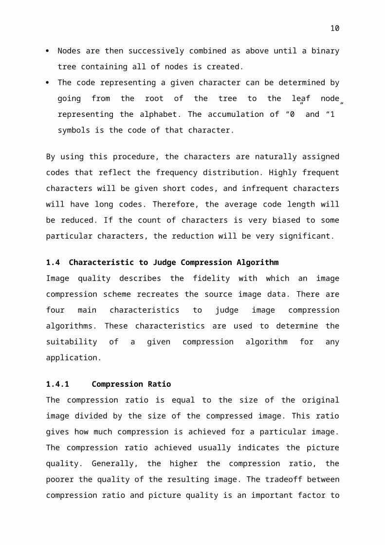
1.4.1 Compression Ratio

The compression ratio is equal to the size of the original image divided by the size of the

compressed image. This ratio gives how much compression is achieved for a particular image.

The compression ratio achieved usually indicates the picture quality. Generally, the higher the

compression ratio, the poorer the quality of the resulting image. The tradeoff between

compression ratio and picture quality is an important factor to consider when compressing

images. Some compression schemes produce compression ratios that are highly dependent on

the image content. This aspect of compression is called data dependency. Using an algorithm

with a high degree of data dependency, an image of a crowd at a football game (which

contains a lot of detail) may produce a very small compression ratio, whereas an image of a

blue sky (which consists mostly of constant colors and intensities) may produce a very high

compression ratio [5].

Amount of original dataCR = (1.1)

7

Amount of compressed data

CR%= (1 - (1/CR))*100 (1.2)

Where CR is compression rate, CR% is compression ratio in percentage.

1.4.2 Compression Speed

Compression time and decompression time are defined as the amount of time required to

compress and decompress a image, respectively. Their value depends on the following

considerations:

The complexity of the compression algorithm.

The efficiency of the software or hardware implementation of the algorithm.

The speed of the utilized processor or auxiliary hardware.

Generally, the faster that both operations can be performed, the better. Fast compression time

increases the speed with which material can be created. Fast decompression time increases the

speed with which the user can display and interact with images [6].

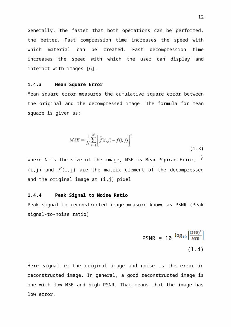
1.4.3 Mean Square Error

Mean square error measures the cumulative square error between the original and the

decompressed image. The formula for mean square is given as:

(1.3)

Where N is the size of the image, MSE is Mean Squrae Error, (i,j) and (i,j) are the matrix

element of the decompressed and the original image at (i,j) pixel

.1.4.4 Peak Signal to Noise Ratio

Peak signal to reconstructed image measure known as PSNR (Peak signal-to-noise ratio)

PSNR = 10 (1.4)

8

Here signal is the original image and noise is the error in reconstructed image. In general, a

good reconstructed image is one with low MSE and high PSNR. That means that the image

has low error.

1.5 Lossless and Lossy Compression

There are two types of image compression they are called lossy and lossless. Lossless image

compression is one of the preferred once and it is used for medical images, architectural

designs and clipart. The reason is that lossless can be converted to its original replica after

compression without losing any data from the image [5]. Second, lossy image compression is

unnoticeable data loss in the image data which is called visually lossless. The data that has

been lost is not visually noticeable to naked eye.

1.5.1 Lossless Compression

It is generally used for applications that cannot allow any difference between the original and

reconstructed data.

1.5.1.1 Run Length Encoding

The adjacent pixels in a typical image are highly correlated. Often it is observed that the

consecutive pixels in a smooth region of an image are identical or the variation among the

neighboring pixels is very small. Appearance of runs of identical values is particularly true for

binary images where usually the image consists of runs of 0's or 1's. Even if the consecutive

pixels in grayscale or color images are not exactly identical but slowly varying, it can often be

pre-processed and the consecutive processed pixel values become identical.

If there is a long run of identical pixels, it is more economical to transmit the length of the run

associated with the particular pixel value instead of encoding individual pixel values [6]. Run-

length coding is a simple approach to source coding when there exists a long run of the same

data, in a consecutive manner, in a data set. As an example, the data d = 4 4 4 4 4 4 4 19 19 19

19 19 19 19 19 19 19 19 19 2 2 2 2 2 2 2 2 11 11 11 11 11 11 contains long runs of 4’s, 19’s,

2’s, 11’s etc. Rather than coding each sample in the run individually, the data can be

represented compactly by simply indicating the value of the sample and the length of its run

when it appears.

9

In this manner the data d can be run-length encoded as (4 7) (19 12) (2 8) (11 6). Here the first

value represents the pixel, while the second indicates the length of its run. In some cases, the

appearance of runs of symbols may not be very apparent. But the data can possibly be pre-

processed in order to aid run-length coding. Consider the data d = 26 29 32 35 38 41 44 50 56

62 68 78 88 98 108 118 116 114 112 110 108 106 104 102 100 98 96.

A simple pre-process on this data, by taking the sample difference e (i) = d (i) – d (i-1), to

produce the processed data e’ = 26 3 3 3 3 3 3 3 6 6 6 6 10 10 10 10 10 -2 -2 -2 -2 -2 -2 -2 -2 -

2 -2 -2. This pre-processed data can now be easily run-length encoded as (26 1) (3 6) (6 4) (10

5) (-2 11). A variation of this technique is applied in the baseline JPEG standard for still-

picture compression.

1.5.1.2 Arithmetic Coding

Arithmetic coding can code more than one symbol with a single code word, thereby allowing

arithmetic coding to achieve a lower bit rate than any variable length coding technique.

Huffman coding was considered the best symbol coding technique, until arithmetic coding

invention; It is able to compress strings of symbols better than Huffman coding. The

arithmetic coding algorithm is better suited to using adaptive statistical models. In other

words, arithmetic coding can adapt to changing symbol probabilities from a source. With an

adaptive statistical model, the symbol probabilities are determined while the symbols are

being coded instead of being determined beforehand as with the Huffman algorithm.

Arithmetic coding is also more computationally efficient than Huffman coding. Huffman

decoding can be computationally expensive since, with each bit read from a compressed file,

the decoder must scan through a look-up table containing the symbol codes [7].

However, with the arithmetic compression program coding and decoding is performed

through integer multiplication and division which is very fast on modem computers. Also

with arithmetic coding, symbols from different sources can easily be encoded mixed together

without loss of compression efficiency [8].

1.5.1.3 Lempel- Ziv - Welch (LZW) Encoding

LZW is a universal lossless data compression algorithm created by Abraham Lempel, Jacob

Ziv, and Terry Welch. It was published by Welch in 1984 as an improved implementation of

the LZ78 algorithm published by Lempel and Ziv in 1978. The algorithm is simple to

implement, and has the potential for very high throughput in hardware implementations [9].

10

LZW compression replaces strings of characters with single codes. It does not do any analysis

of the incoming text. Instead, it just adds every new string of characters to a table of strings.

Compression occurs when a single code is output instead of a string of characters. The code

that the LZW algorithm output can be of any arbitrary length, but it must have more bits in it

than a single character. The first 256 codes when using eight bit characters are by default

assigned to the standard character set. The remaining codes are assigned to strings as the

algorithm proceeds.

1.5.1.4 Chain Codes

A chain code is a lossless compression algorithm for monochrome images. The basic

principle of chain codes is to separately encode each connected component in the image.

For each such region, a point on the boundary is selected and its coordinates are transmitted.

The encoder then moves along the boundary of the region and, at each step, transmits a

symbol representing the direction of this movement. This continues until the encoder returns

to the starting position, at which point the pixel has been completely described, and encoding

continues with the next pixel in the image [6].

This encoding method is particularly effective for images consisting of a reasonably small

number of large connected components.

1.5.2 Lossy Compression

Lossy compression techniques involve some loss of information, and data cannot be re-

covered or reconstructed exactly. In some applications, exact reconstruction is not necessary.

For example, it is acceptable that a reconstructed video signal is different from the original as

long as the differences do not result in annoying artifacts.

1.5.2.1 Quantization

Quantization is a lossy compression technique achieved by compressing a range of values to a

single quantum value. When the number of discrete symbols in a given stream is reduced, the

stream becomes more compressible. For example, reducing the number of colors required to

represent a digital image makes it possible to reduce its file size. Specific applications include

DCT (Discrete cosine transform) data quantization in JPEG and DWT (Discrete wavelet

transform) data quantization in JPEG 2000 [10].

11

There are two types of quantization - Vector Quantization and Scalar Quantization. Vector

quantization (VQ) is similar to scalar quantization except that the mapping is performed on

vectors or blocks of pixels rather than on individual pixels [11]. The general VQ algorithm

has three main steps. First the image is partitioned into blocks which are usually 2X2or 4X4

in size. After blocking the image, a codebook which best estimates the blocks of the image is

constructed and indexed. Finally, the original image blocks are substituted by the index of

best estimate code from the codebook.

1.5.2.2 Predictive Coding

It is a tool used mostly in audio signal processing and speech processing for representing the

spectral envelope of a digital signal of speech in compressed form, using the information of a

linear predictive model.

It is one of the most powerful speech analysis techniques, and one of the most useful methods

for encoding good quality speech at a low bit rate and provides extremely accurate estimates

of speech parameters [12].

1.5.2.3 Fractal Compression

Fractal compression is a lossy compression method for digital images, based on fractals. The

method is best suited for textures and natural images, relying on the fact that parts of an image

often resemble other parts of the same image. Fractal algorithms convert these parts into

mathematical data called "fractal codes" which are used to recreate the encoded image [6].

With fractal compression, encoding is extremely computationally expensive because of the

search used to find the self-similarities. Decoding however is quite fast. While this asymmetry

has so far made it impractical for real time applications, when video is archived for

distribution from disk storage or file downloads fractal compression becomes more

competitive.

1.5.2.4 Wavelet Transform

Mathematically a “wave” is expressed as a sinusoidal (or oscillating) function of time or

space. Fourier analysis expands an arbitrary signal in terms of infinite number of sinusoidal

functions of its harmonics. Fourier representation of signals is known to be very effective in

analysis of time-invariant (stationary) periodic signals. In contrast to a sinusoidal function, a

wavelet is a small wave whose energy is concentrated in time. Properties of wavelets allow

both time and frequency analysis of signals simultaneously because of the fact that the energy

12

of wavelets is concentrated in time and still possesses the wave-like (periodic) characteristics.

Wavelet representation thus provides a versatile mathematical tool to analyze transient, time-

variant (nonstationary) signals that may not be statistically predictable especially at the region

of discontinuities a special feature that is typical of images having discontinuities at the edges

[13].

Transform coding of images is performed by the projection of an image on some basis. The

basis is chosen so that the projection will effectively decorrelate the pixel values, and thus,

represent the image in a more compact form. The transformed (decomposed) image is then

quantized and coded using different methods such as scalar and vector quantization,

arithmetic coding, run length coding, Huffman coding, and others.

1.6 The Use of Neural and Wavelet Techniques for Image Compression

With the growth of multimedia and internet, compression techniques have become the thrust

area in the fields of computers. Multimedia combines many data types like text, graphics,

images, animation, audio and video. Image compression is a process of efficiently coding

digital image to reduce the number of bits required in representing images. Its purpose is to

reduce the storage space and transmission cost while maintaining good quality. Many

different image compression techniques currently exist for the compression of different types

of images. In [16] back propagation neural network training algorithm has been used for

image compression. Back propagation neural network algorithm helps to increase the

performance of the system and to decrease the convergence time for the training of the neural

network.

The aim of this work is to develop an edge preserving image compressing technique using

one hidden layer feed forward neural network of which the neurons are determined adaptively

.The processed image block is fed as a single input pattern while single output pattern has

been constructed from the original image unlike other neural network based technique where

multiple image blocks are fed to train the network.

In [17] an adaptive method for image compression based on complexity level of the image

and modification on levenberg-marquardt algorithm for MLP neural network learning is used.

In adaptive method different back propagation artificial neural networks are used as

compressor and de-compressor and it is achieved by dividing the image into blocks,

computing the complexity of each block and then selecting one network for each block

13

according to its complexity value. The proposed algorithm has good convergence. This

method reduces the amount of oscillation in learning procedure.

Multilayer neural network (MLP) is employed to achieve image compression in [23]. The

network parameters are adjusted using different learning rules for comparison purposes.

Mainly, the input pixels will be used as target values so that assigned mean square error can

be obtained, and then the hidden layer output will be the compressed image. It was noticed

that selection between learning algorithms is important as a result of big variations among

them with respect to convergence time and accuracy of results.

After decomposing an image using the discrete wavelet transforms (DWT), a neural network

may be able to represent the DWT coefficients in less space than the coefficients themselves

[15]. After splitting the image and the decomposition using several methods, neural networks

were trained to represent the image blocks. By saving the weights and bias of each neuron, an

image segment can be approximately recreated. Compression can be achieved using neural

networks. Current results have been promising except for the amount of time needed to train a

neural network.

Wavelet network is the tight combination of wavelet decomposition and neural network,

where wavelet basis function works as the activation function. In [18] Wavelet network is

used to compress images in this paper the comparison between wavelet network and

traditional neural network is presented. The result shows that wavelet network method

succeeded in improving performances and efficiency in image compression.

[27] Discusses important features of wavelet transform in compression of still images,

including the extent to which the quality of image is degraded by the process of wavelet

compression and decompression. Image quality is measured objectively, using peak signal-to-

noise ratio or picture quality scale, and subjectively, using perceived image quality. The

effects of different wavelet functions, image contents and compression ratios are assessed. A

comparison with a discrete-cosine transform-based compression system is given. His results

provide a good reference for application developers to choose a good wavelet compression

system for their application.

Image compression is now essential for applications such as transmission and storage in data

bases. [3] Review and discuss about the image compression, need of compression, its

principles, and classes of compression and various algorithm of image compression. [3]

14

Attempts to give a recipe for selecting one of the popular image compression algorithms

based on Wavelet, JPEG/DCT, VQ, and Fractal approaches. He reviews and discuss the

advantages and disadvantages of these algorithms for compressing grayscale images, give an

experimental comparison on 256×256 commonly used image of Lena and one 400×400

fingerprint image.

[26] Describes a method of encoding an image without blocky effects. The method

incorporates the wavelet transform and a self development neural network-Vitality

Conservation (VC) network to achieve significant improvement in image compression

performance. The implementation consists of three steps. First, the image is decomposed at

different scales using wavelet transform to obtain an orthogonal wavelet representation of the

image. Each band can be subsequently processed in parallel. At the second step, the discrete

Karhunen-Loeve transform is used to extract the principal components of the wavelet

coefficients. Thus, the processing speed can be much faster than otherwise. Finally, results of

the second step are used as input to the VC network for vector quantization our simulation

results show that such implementation can; achieve superior reconstructed images to other

methods, in much less time.

[28] Proposes a neuro- wavelet based model for image compression which combines the

advantage of wavelet transform and neural network. Images are decomposed using wavelet

filters into a set of sub bands with different resolution corresponding to different frequency

bands. Different quantization and coding schemes are used for different sub bands based on

their statistical properties. The coefficients in low frequency band are compressed by

differential pulse code modulation (DPCM) and the coefficients in higher frequency bands are

compressed using neural network. Using this scheme we can achieve satisfactory

reconstructed images with large compression ratios.

For many years, there are increasing growth in the need of numeric pictures (whether

stationary or animate) in numerous fields such as telecommunications, multimedia diffusion,

medical diagnosis, telesurveillance, meteorology, robotics, etc. However, this type of data

represents a huge mass of information that is difficult to transmit and to stock with the current

means. Thus, it was necessary to have new techniques that rely on the efficiency of images

compression. Recent researches on images compression have shown an increasing interest

toward exploiting the power of wavelet transforms and neural networks to improve the

compression efficiency. [19] Has chosen to implement a new approach combining both

15

wavelets and neural networks (and called wavelet networks). The results are compared to

some classical MLP neural networks techniques and to other schemes of networks depending

on the wavelets used in the hidden layer, the number of these wavelets and the number of

iterations. The obtained results perfectly matches the results from the experiments mentioned

in the paper, which prove that wavelet networks outperform neural networks in term of both

compression ratio and quality of the reconstructed images.

[20] Presents a new image compression scheme which uses the wavelet transform and neural

networks. Image compression is performed in three steps. First, the image is decomposed at

different scales, using the wavelet transform, to obtain an orthogonal wavelet representation

of the image. Second, the wavelet coefficients are divided into vectors, which are projected

onto a subspace using a neural network. The number of coefficients required to represent the

vector in the subspace is less than the number of coefficients required to represent the original

vector, resulting in data compression. Finally, the coefficients which project the vectors of

wavelet coefficients onto the subspace are quantized and entropy coded.

The need for an efficient technique for compression of Images ever increasing because the

raw images need large amounts of disk space seems to be a big disadvantage during

transmission & storage. Even though there are so many compression techniques already

present a better technique which is faster, memory efficient and simple surely suits the

requirements of the user. [5] proposed the Lossless method of image compression and

decompression using a simple coding technique called Huffman coding. This technique is

simple in implementation and utilizes less memory. A software algorithm has been developed

and implemented to compress and decompress the given image using Huffman coding

techniques in a MATLAB platform.

1.7 Summary

In this chapter, the methodologies used for data compression are described. Commonly used

compression algorithms including both lossless and lossy comporisions are presented. The

characteristics of compression algorithms and the use of neural and wavelet technologies for

image compression are given.

16

CHAPTER TWO

NEURAL NETWORK STRUCTURE FOR IMAGE COMPRESSION

2.1 Overview

In this chapter an introduction to neural network based compressing algorithm is given. The

different structures of neural networks and their supervised and unsupervised training ap-

proaches are given. The learning of neural network based image compression system using

back-propogation algorithm will be described.

2.2 Introduction to Neural Networks

A neural network is a powerful data modeling tool that is able to capture and represent

complex input/output relationships. The motivation for the development of neural network

technology stemmed from the desire to develop an artificial system that could perform

"intelligent" tasks similar to those performed by the human brain. Neural networks resemble

the human brain in the following two ways:

A neural network acquires knowledge through learning.

A neural network's knowledge is stored within inter-neuron connection strengths known

as synaptic weights.

Artificial Neural Networks are being counted as the wave of the future in computing. They

are indeed self learning mechanisms which don't require the traditional skills of a programmer

[14]. Neural networks are a set of neurons connected together in some manner. These neurons

can contain separate transfer functions and have individual weights and biases to determine an

output value based on the inputs. An example of a basic linear neuron can be thought of as a

function which takes several inputs, multiplies each by its respective weight, adds an overall

bias and outputs the result. Other types of neurons exist and there are many methods with

which to train a neural network. Training implies modifying the weights and bias of each

17

neuron until an acceptable output goal is reached. During training, if the output is far from its

desired target, the weights and biases are changed to help achieve a lower error [15].

A biological neural network is composed of a group or groups of chemically connected or

functionally associated neurons. A single neuron may be connected to many other neurons

and the total number of neurons and connections in a network may be extensive. Connections,

called synapses, are usually formed from axons to dendrites, though dendro dendritic

microcircuits and other connections are possible. Apart from the electrical signaling, there are

other forms of signaling that arise from neurotransmitter diffusion, which have an effect on

electrical signaling. As such, neural networks are extremely complex.

2.3 Neural Networks versus Conventional Computers

Neural networks take a different approach to problem solving than that of conventional com-

puters.

Conventional computers use an algorithmic approach i.e., the computer follows a set of

instructions in order to solve a problem. Unless the specific steps that the computer needs to

follow are known the computer cannot solve the problem. That restricts the problem solving

capability of conventional computers to problems that we already understand and know how

to solve. But computers would be so much more useful if they could do things that we don't

exactly know how to do [16].

Neural networks on the other hand, process information in a similar way the human brain

does. The network is composed of a large number of highly interconnected processing

elements (neurons) working in parallel to solve a specific problem. Neural networks learn by

training. They cannot be programmed to perform a specific task [17]. The disadvantage of

neural networks is that because the network finds out how to solve the problem by itself; its

operation can be unpredictable. On the other hand, conventional computers use a cognitive

approach to problem solving, the way the problem is to be solved must be known and stated

in small unambiguous instructions.

These instructions are then converted to a high level language program and then into machine

code that the computer can understand. These machines are totally predictable, if anything

goes wrong is due to a software or hardware fault. Neural networks and conventional

algorithmic computers are not in competition but complement each other. There are tasks that

are more suited to an algorithmic approach like arithmetic operations and tasks that are more

18

suited to neural networks. Even more, a large number of tasks require systems that use a

combination of the two approaches (normally a conventional computer is used to supervise

the neural network) in order to perform at maximum efficiency.

2.4 Neural Network Architecture

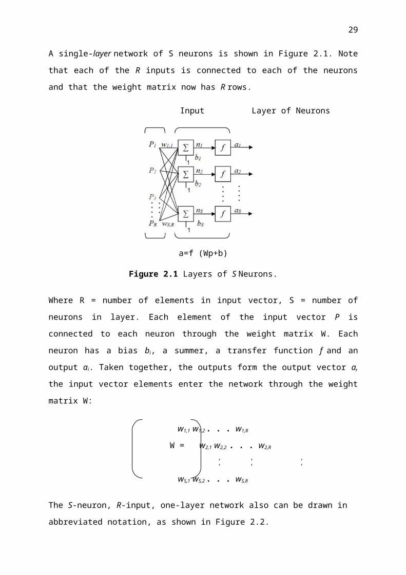
A single-layer network of S neurons is shown in Figure 2.1. Note that each of the R inputs is

connected to each of the neurons and that the weight matrix now has R rows.

Input Layer of Neurons

a=f (Wp+b)

Figure 2.1 Layers of S Neurons.

Where R = number of elements in input vector, S = number of neurons in layer. Each element

of the input vector P is connected to each neuron through the weight matrix W. Each neuron

has a bias bi, a summer, a transfer function f and an output ai. Taken together, the outputs

form the output vector a, the input vector elements enter the network through the weight

matrix W:

w1,1 w1,2 . . . w1,R

W = w2,1 w2,2 . . . w2,R

wS,1 wS,2 . . . wS,R

The S-neuron, R-input, one-layer network also can be drawn in abbreviated notation, as

shown in Figure 2.2.

19

Figure 2.2 Layers of S Neurons, Abbreviated Notation [14].

Here again, the symbols below the variables tell you that for this layer, P is a vector of length

R, W is a matrix, a and b are vectors of length S. The layer includes the weight matrix, the

summation and multiplication operations, the bias vector b, the transfer function boxes and

the output vector.

2.4.1 Multiple Layers of Neurons

Now consider a network with several layers. Each layer has its own weight matrix W, its own

bias vector b, a net input vector n and an output vector a, We need to introduce some

additional notation to distinguish between these layers. We will use superscripts to identify

the layers. Thus, the weight matrix for the first layer is written as W1, and the weight matrix

for the second layer is written as W2. This notation is used in the three-layer network shown in

Figure 2.4 As shown, there are R inputs, S1 neurons in the first layer, S2 neurons in the second

layer, etc. As noted, different layers can have different numbers of neurons [18][19].

Connections Hidden Layers

Input Layer

Output Layer

Figure 2.3 Multilayers Neural Networks

20

The outputs of layers one and two are the inputs for layers two and three. Thus layer 2 can be

viewed as a one-layer network with R=S1inputs, S=S2 neurons, and an S2xS1 weight matrix

W2 the input to layer 2 is a1, and the output is a2.

A layer whose output is the network output is called an output layer. The other layers are

called hidden layers. The network shown in Figure 2.4 has an output layer (layer 3) and two

hidden layers (layers 1 and 2).

Figure 2.4 Three-Layer Networks [14].

2.5 Training an Artificial Neural Network

The brain basically learns from experience. Neural networks are sometimes called machine-

learning algorithms, because changing of its connection weights (training) causes the network

to learn the solution to a problem. The strength of connection between the neurons is stored as

a weight-value for the specific connection. The system learns new knowledge by adjusting

these connection weights [20].

The learning ability of a neural network is determined by its architecture and by the

algorithmic method chosen for training. The training method usually consists of two schemes:

2.5.1 Supervised Learning

The majority of artificial neural network solutions have been trained with supervision. In this

mode, the actual output of a neural network is compared to the desired output. Weights, which

are usually randomly set to begin with, are then adjusted by the network so that the next

iteration, or cycle, will produce a closer match between the desired and the actual output. The

learning method tries to minimize the current errors of all processing elements.

21

This global error reduction is created over time by continuously modifying the input weights

until acceptable network accuracy is reached. With supervised learning, the artificial neural

network must be trained before it becomes useful. Training consists of presenting input and

output data to the network. This data is often referred to as the training set. That is, for each

input set provided to the system, the corresponding desired output set is provided as well. This

training is considered complete when the neural network reaches a user defined performance

level [21].

This level signifies that the network has achieved the desired statistical accuracy as it

produces the required outputs for a given sequence of inputs. When no further learning is

necessary, the weights are typically frozen for the application. Training sets need to be fairly

large to contain all the needed information. Not only do the sets have to be large but the

training sessions must include a wide variety of data.

After a supervised network performs well on the training data, then it is important to see what

it can do with data it has not seen before. If a system does not give reasonable outputs for this

test set, the training period is not over. Indeed, this testing is critical to insure that the network

has not simply memorized a given set of data but has learned the general patterns involved

within an application.

2.5.2 Unsupervised Learning

Unsupervised learning is the great promise of the future. It shouts that computers could

someday learn on their own in a true robotic sense. Currently, this learning method is limited

to networks known as self organizing maps.

Training algorithms that adjust the weights in a neural network by reference to a training data

set including input variables only. Unsupervised learning algorithms attempt to locate clusters

in the input data. The hidden neurons must find a way to organize themselves without help

from the outside. In this approach, no sample outputs are provided to the network against

which it can measure its predictive performance for a given vector of inputs. This is learning

by doing [22].

An unsupervised learning algorithm might emphasize cooperation among clusters of processing elements. In such a scheme, the clusters would work together. If some external input activated any node in the cluster, the cluster's activity as a whole could be increased. Likewise, if external

22

input to nodes in the cluster was decreased, that could have an inhibitory effect on the entire cluster.

Competition between processing elements could also form a basis for learning. Training of

competitive clusters could amplify the responses of specific groups to specific stimuli. As

such, it would associate those groups with each other and with a specific appropriate

response. Normally, when competition for learning is in effect, only the weights belonging to

the winning processing element will be updated.

At the present state of the art, unsupervised learning is not well understood and is still the

subject of research. This research is currently of interest to the government because military

situations often do not have a data set available to train a network until a conflict arises.

2.6 Back-propagation Training Algorithm

Back-propagation is a technique discovered by Rumelhart, Hinton and Williams in 1986 and

it is a supervised algorithm that learns by first computing the output using a feed forward net-

work, then calculating the error signal and propagating the error backwards through the net-

work.

With back-propagation algorithm, the input data is repeatedly presented to the neural network.

With each presentation the output of the neural network is compared to the desired output and

an error is computed. This error is then feedback (back-propagated) to the neural network and

used to adjust the weights such that the error decreases with each iteration and the neural

model gets closer and closer to producing the desired output. This process is known as "train-

ing" [23].

The back-propagation algorithm is perhaps the most widely used training algorithm for multi-

layered feed-forward networks. However, many people find it quite difficult to construct mul-

tilayer feed-forward networks and training algorithms, whether it is because of the difficulty

of the math or the difficulty involved with the actual coding of the network and training al-

gorithm.

Multilayer feed-forward networks normally consist of three or four layers, there is always one

input layer and one output layer and usually one hidden layer, although in some classification

problems two hidden layers may be necessary, this case is rare however.

23

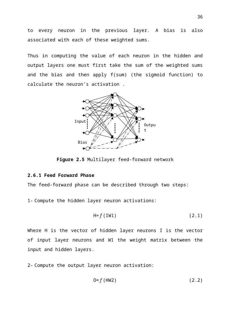
In a fully connected multilayer feed-forward network (See Figure 2.5), each neuron in one

layer is connected by a weight to every neuron in the previous layer. A bias is also associated

with each of these weighted sums.

Thus in computing the value of each neuron in the hidden and output layers one must first

take the sum of the weighted sums and the bias and then apply f(sum) (the sigmoid function)

to calculate the neuron's activation .

Figure 2.5 Multilayer feed-forward network

2.6.1 Feed Forward Phase

The feed-forward phase can be described through two steps:

1- Compute the hidden layer neuron activations:

H= f (IW1) (2.1)

Where H is the vector of hidden layer neurons I is the vector of input layer neurons and W1

the weight matrix between the input and hidden layers.

2- Compute the output layer neuron activation:

O= f (HW2) (2.2)

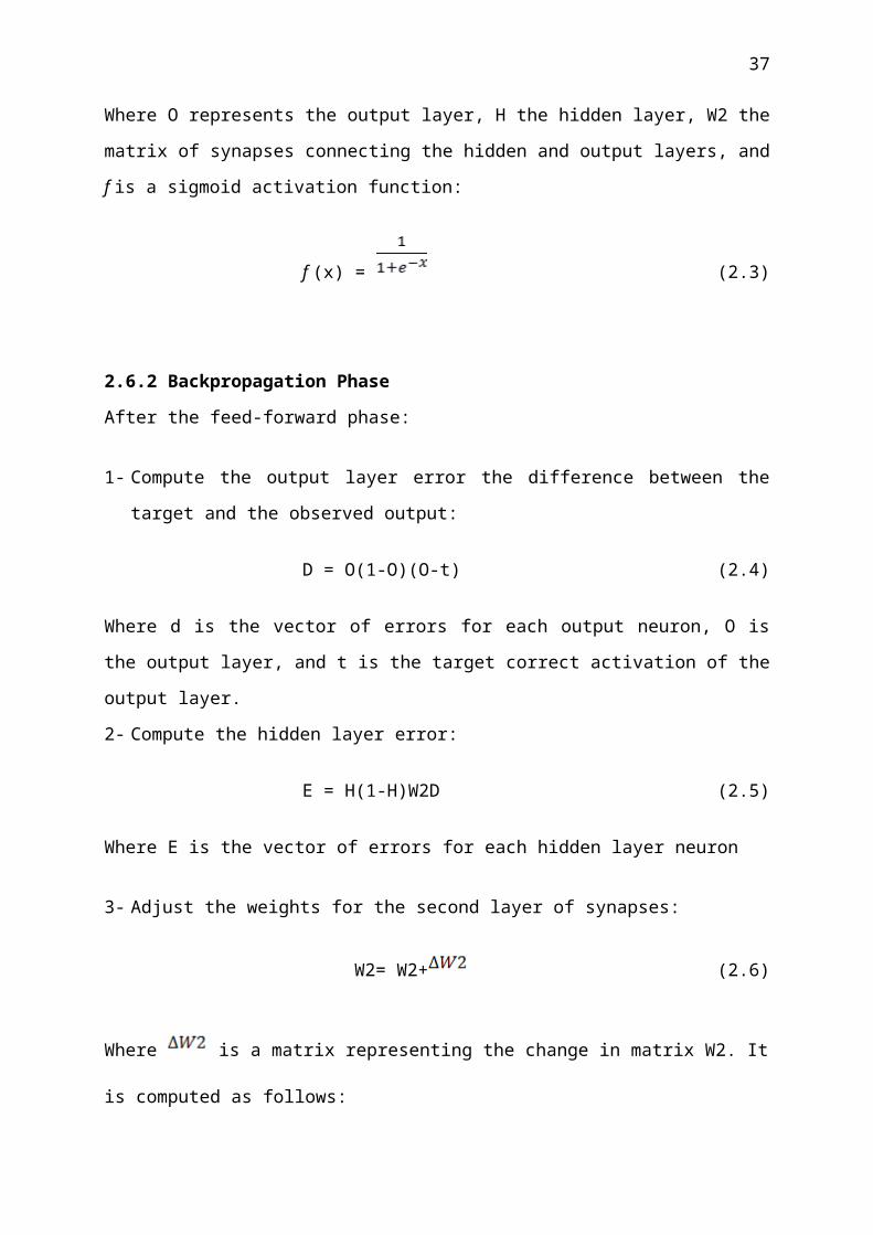
Where O represents the output layer, H the hidden layer, W2 the matrix of synapses

connecting the hidden and output layers, and f is a sigmoid activation function:

f (x) = (2.3)

Bias

InputOutput

24

2.6.2 Backpropagation Phase

After the feed-forward phase:

1- Compute the output layer error the difference between the target and the observed output:

D = O(1-O)(O-t) (2.4)

Where d is the vector of errors for each output neuron, O is the output layer, and t is the target

correct activation of the output layer.

2- Compute the hidden layer error:

E = H(1-H)W2D (2.5)

Where E is the vector of errors for each hidden layer neuron

3- Adjust the weights for the second layer of synapses:

W2= W2+ (2.6)

Where is a matrix representing the change in matrix W2. It is computed as follows:

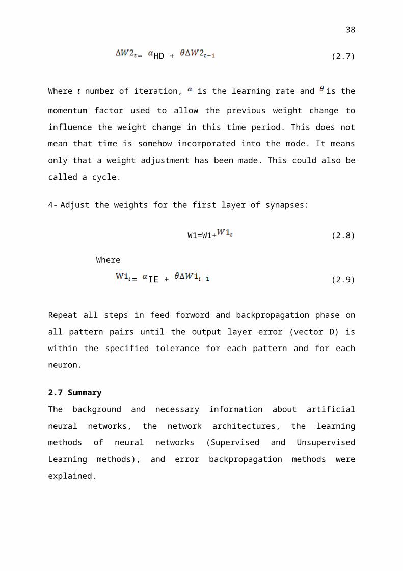
= HD + (2.7)

Where t number of iteration, is the learning rate and is the momentum factor used to

allow the previous weight change to influence the weight change in this time period. This

does not mean that time is somehow incorporated into the mode. It means only that a weight

adjustment has been made. This could also be called a cycle.

4- Adjust the weights for the first layer of synapses:

W1=W1+ (2.8)

Where

= IE + (2.9)

25

Repeat all steps in feed forword and backpropagation phase on all pattern pairs until the

output layer error (vector D) is within the specified tolerance for each pattern and for each

neuron.

2.7 Summary

The background and necessary information about artificial neural networks, the network

architectures, the learning methods of neural networks (Supervised and Unsupervised

Learning methods), and error backpropagation methods were explained.

CHAPTER THREE

WAVELET TRANSFORM FOR IMAGE COMPRESSION

3.1 Overview

In this chapter the mathematical model of wavelet transform is given. The power of wavelet

analysis is explained. The multiresolution analysis of wavelet, discrete wavelet transform will

be described. The DWT subsignal encoding and decoding and an example of multiresolution

analysis of wavelet for image compression shall be demonstrated.

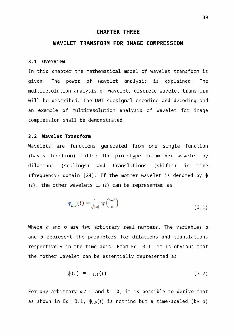
3.2 Wavelet Transform

Wavelets are functions generated from one single function (basis function) called the

prototype or mother wavelet by dilations (scalings) and translations (shifts) in time

(frequency) domain [24]. If the mother wavelet is denoted by ψ (t), the other wavelets ψa,b(t)

can be represented as

(3.1)

Where a and b are two arbitrary real numbers. The variables a and b represent the parameters

for dilations and translations respectively in the time axis. From Eq. 3.1, it is obvious that the

mother wavelet can be essentially represented as

ψ(t) = ψ1,0(t) (3.2)

26

For any arbitrary a ≠ 1 and b = 0, it is possible to derive that as shown in Eq. 3.1, ψa,0(t) is

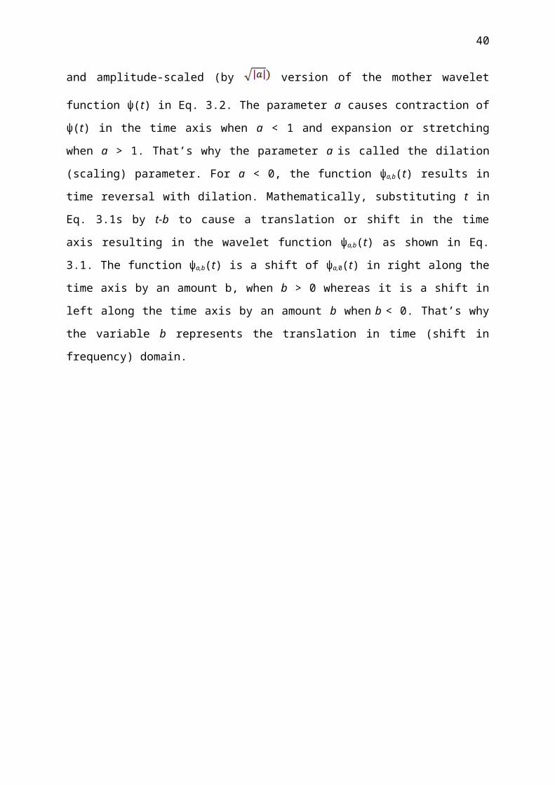
nothing but a time-scaled (by a) and amplitude-scaled (by version of the mother

wavelet function ψ(t) in Eq. 3.2. The parameter a causes contraction of ψ(t) in the time axis

when a < 1 and expansion or stretching when a > 1. That’s why the parameter a is called the

dilation (scaling) parameter. For a < 0, the function ψa,b(t) results in time reversal with

dilation. Mathematically, substituting t in Eq. 3.1s by t-b to cause a translation or shift in the

time axis resulting in the wavelet function ψa,b(t) as shown in Eq. 3.1. The function ψa,b(t) is a

shift of ψa,0(t) in right along the time axis by an amount b, when b > 0 whereas it is a shift in

left along the time axis by an amount b when b < 0. That’s why the variable b represents the

translation in time (shift in frequency) domain.

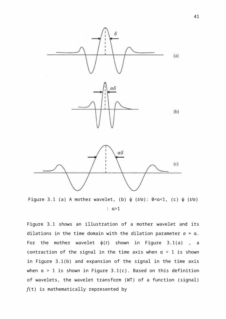
Figure 3.1 (a) A mother wavelet, (b) ψ (t/a): 0<α<1, (c) ψ (t/a) : α>1

27

Figure 3.1 shows an illustration of a mother wavelet and its dilations in the time domain with

the dilation parameter a = α. For the mother wavelet ψ(t) shown in Figure 3.1(a) , a

contraction of the signal in the time axis when α < 1 is shown in Figure 3.1(b) and expansion

of the signal in the time axis when α > 1 is shown in Figure 3.1(c). Based on this definition of

wavelets, the wavelet transform (WT) of a function (signal) f(t) is mathematically represented

by

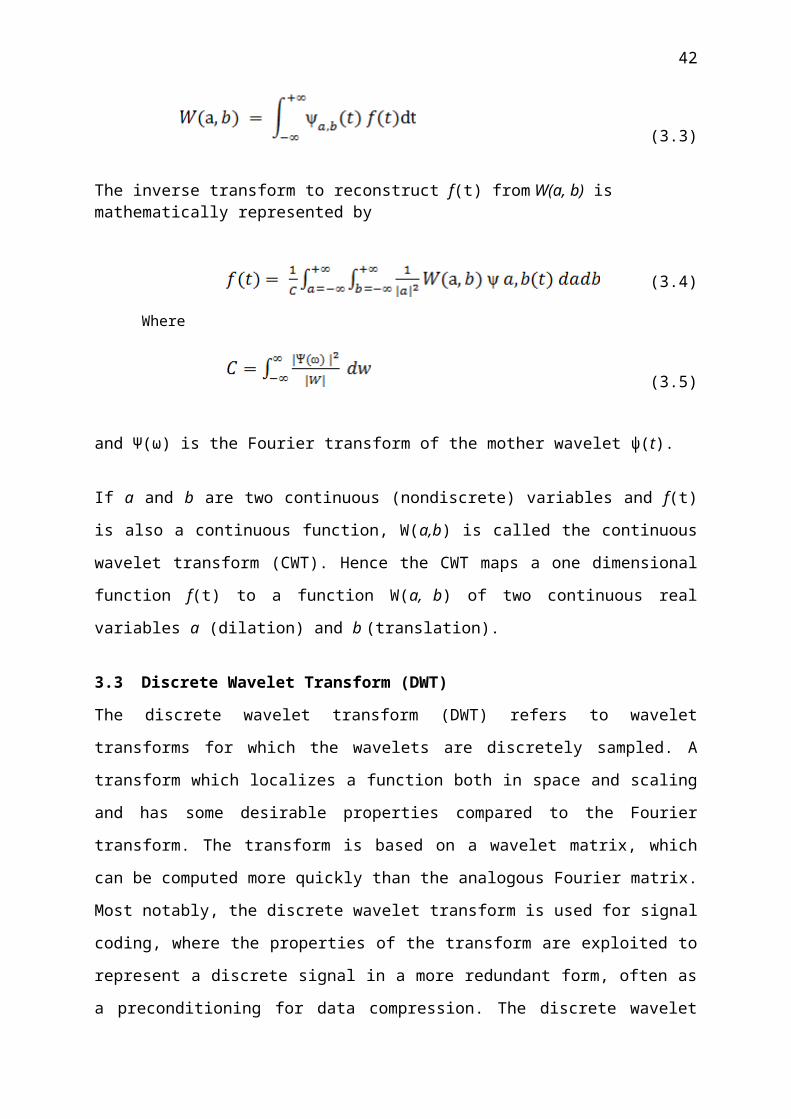
(3.3)

The inverse transform to reconstruct f(t) from W(a, b) is mathematically represented by

(3.4)

Where

(3.5)

and Ψ(ω) is the Fourier transform of the mother wavelet ψ(t).

If a and b are two continuous (nondiscrete) variables and f(t) is also a continuous function,

W(a,b) is called the continuous wavelet transform (CWT). Hence the CWT maps a one

dimensional function f(t) to a function W(a, b) of two continuous real variables a (dilation)

and b (translation).

3.3 Discrete Wavelet Transform (DWT)

The discrete wavelet transform (DWT) refers to wavelet transforms for which the wavelets

are discretely sampled. A transform which localizes a function both in space and scaling and

has some desirable properties compared to the Fourier transform. The transform is based on a

wavelet matrix, which can be computed more quickly than the analogous Fourier matrix.

Most notably, the discrete wavelet transform is used for signal coding, where the properties of

the transform are exploited to represent a discrete signal in a more redundant form, often as a

preconditioning for data compression. The discrete wavelet transform has a huge number of

applications in Science, Engineering, Mathematics and Computer Science [25][26].

28

Wavelet compression is a form of data compression well suited for image compression

(sometimes also video compression and audio compression). The goal is to store image data

in as little space as possible in a file. A certain loss of quality is accepted (lossy compression).

Signal can be represented by a smaller amount of information than would be the case if some

other transform, such as the more widespread discrete cosine transform, had been used.

First a wavelet transform is applied. This produces as many coefficients as there are pixels in

the image (i.e., there is no compression yet since it is only a transform). These coefficients

can then be compressed more easily because the information is statistically concentrated in

just a few coefficients. This principle is called transform coding. After that, the coefficients

are quantized and the quantized values are entropy encoded or run length encoded.

3.4 Multiresolution Analysis

The power of Wavelets comes from the use of multiresolution. Rather than examining entire

signals through the same window, different parts of the wave are viewed through different

size windows (or resolutions). High frequency parts of the signal use a small window to give

good time resolution; low frequency parts use a big window to get good frequency

information [27].

An important thing to note is that the ’windows’ have equal area even though the height and

width may vary in wavelet analysis. The area of the window is controlled by Heisenberg’s

Uncertainty principle, as frequency resolution gets bigger the time resolution must get

smaller.

In Fourier analysis a signal is broken up into sine and cosine waves of different frequencies,

and it effectively re-writes a signal in terms of different sine and cosine waves. Wavelet

analysis does a similar thing, it takes a mother wavelet and then the signal is translated into

shifted and scale versions of this mother wavelet.

3.5 DWT Subsignal Encoding and Decoding

The DWT provides sufficient information for the analysis and synthesis of a signal, but is

advantageously, much more efficient. Discrete Wavelet analysis is computed using the

concept of filter banks. Filters of different cut-off frequencies analyse the signal at different

29

scales. Resolution is changed by filtering; the scale is changed by upsampling and

downsampling. If a signal is put through two filters:

A high-pass filter, high frequency information is kept, low frequency information is lost.

A low pass filter, low frequency information is kept, high frequency information is lost.

The input discrete signal x(n) (shown as a(0,n) in Figure 3.2, it is filtered parallelly by a low

pass (h) and a high-pass (g) at each transform level. The two output streams are then

subsampled by simply dropping the alternate output samples in each stream to produce the

low-pass subband. The low-pass subband a(1, n) is an approximation of the input to produce

the subbands a(2,n) and d(2,n) so on [28]. During the inverse transform to reconstruct the

signal, both a(3,n) and d(3,n) are first upsampled by inserting zeros between two samples, and

then they are filtered by low-pass (h’) and high-pass (g’) filters respectively.

These two filtered output streams are added together to reconstruct a(2,n). The same

continues until the reconstruction of the original signal a(0,n).

Figure 3.2 Three-level multiresolution wavelet decomposition and reconstruction of signals

using filter structure.

3.6 Example of Haar Wavelet Transform

The Haar Transform (HT) is transformations from the space domain to a local frequency do-

main. A HT decomposes each signal into two components, one is called average (approxima-

tion) or trend and the other is known as difference (detail) or fluctuation. A precise formula

for the values of first average subsignal a = (a1,a2 ,...,aN/2) at one level for a signal of length

N i.e. f=( f1, f2,…., fN ) is

30

an = , n = 1,2,3,….,N/2 (3.6)

And the first detail subsignal, d = (d1,d2 ,...,dN/2) at the same level is given as

dn = , n = 1,2,3,….,N/2 (3.7)

For simplicity, to describe the averaging and differencing process we take only the first row

of an 8x8 matrix. This row is shown below. Because our matrix is 8x8 the process will

involve three steps (23 = 8).

[ 3 5 4 8 13 7 5 3 ]

Step 1

For the first step we take the average of each pair of components in our original string and

place the result in the first four positions of our new string. The remaining four numbers are

the differences of the first element in each pair and its corresponding average (e.g. 3 – 5 = -2,

average of -2 = -1, 4 – 8 = -4 average of -4 = -2) these numbers are called detail coefficients.

Our result of the first step therefore contains four averages and four detail coefficients (bold)

as shown below.

[ 4 6 10 4 -1 -2 3 1 ]

Step 2

We then apply this same method to the first four components of our new string resulting in

two new averages and their corresponding detail coefficients. The remaining four detail

coefficients are simply carried directly down from our previous step. And the result for step

two is as follows.

[ 5 7 -1 3 -1 -2 3 1 ]

Step 3

Performing the same averaging and differencing to the remaining pair of averages completes

step three. The last six components have again been carried down from the previous step. We

now have as our string, one row average in the first position followed by seven detail

coefficients.

31

[ 6 -1 -1 3 -1 -2 3 1 ]

3.6.1 Image Representation

We can now use the same averaging and differencing process and apply it to an entire matrix.

The following matrix (A) represents the image in figure 3.3. Notice the larger components in

the matrix represent the lighter shades of gray.

64 2 3 61 60 6 7 57

9 55 54 12 13 51 50 16

17 47 46 20 21 43 42 24

A = 40 26 27 37 36 30 31 33

32 34 35 29 28 38 39 25

41 23 22 44 45 19 18 48

49 15 14 52 53 11 10 56

8 58 59 5 4 62 63 1

Figure 3.3 Represents the image of matrix (A) 8x8.

If we apply the averaging and differencing to each of the rows the results are row averages in

the first column and the remaining components being the detail coefficients of that row.

32.5 0 0.5 0.5 31 -29 27 -25

32.5 0 -0.5 -0.5 23 21 -19 17

32.5 0 -0.5 -0.5 -15 13 -11 9

32.5 0 0.5 0.5 7 -5 3 -1

32.5 0 0.5 0.5 -1 3 -5 7

32.5 0 -0.5 -0.5 9 -11 13 -15

32

32.5 0 -0.5 -0.5 17 -19 21 -23

32.5 0 0.5 0.5 -27 27 -29 31

If we now apply the averaging and differencing to the columns we get the following matrix.

32.5 0 0 0 0 0 0 0

0 0 0 0 0 0 0 0

0 0 0 0 4 - 4 4 - 4

0 0 0 0 4 - 4 4 4

0 0 0.5 0.5 27 -25 23 -21

0 0 -0.5 -0.5 -11 9 -7 5

0 0 0.5 0.5 -5 7 -9 11

0 0 -0.5 -0.5 21 -23 25 -27

We now have a matrix that represents our image in a more concise manner: with on overall

average in the upper left – hand corner of the matrix. The remaining components are all detail

coefficients that now represent the amount of detail in that area of the image. Because we

know this, we can eliminate some information from our matrix and still be capable of

attaining a fairly good approximation of our original matrix. Doing this we choose some

number ( ) and set equal to zero all elements with a magnitude less than .

Choosing = | 5 | we eliminated eighteen of the detail coefficients (bold).

32.5 0 0 0 0 0 0 0

0 0 0 0 0 0 0 0

0 0 0 0 0 0 0 0

0 0 0 0 0 0 0 0

0 0 0 0 27 -25 23 -21

0 0 0 0 -11 9 -7 0

0 0 0 0 0 7 -9 11

0 0 0 0 21 -23 25 -27

To arrive at our approximation of the original matrix we now apply the inverse of the

averaging and differencing operations.

33

59.5 5.5 7.5 57.5 55.5 9.5 11.5 53.5

5.5 59.5 57.5 7.5 9.5 55.5 53.5 11.5

21.5 43.5 41.5 23.5 25.5 39.5 32.5 32.5

43.5 21.5 23.5 41.5 39.5 25.5 32.5 32.5

32.5 32.5 39.5 25.5 23.5 41.5 21.5 21.5

32.5 32.5 25.5 39.5 41.5 23.5 43.5 43.5

53.5 11.5 9.5 55.5 57.5 7.5 5.5 59.5

11.5 53.5 55.5 9.5 7.5 57.5 59.5 5.5

As shown in figure 3.4 we can get a good approximation of the original image by using this

process. We have lost some of the details in the image, but it is so minimal that the loss would

not be noticeable in most cases.

Original Image Decompressed Image

Figure 3.4 Represents the original and decompressed image of matrix (A).

3.7 Summary

The mathematical background of wavelet transform, the discreate wavelet transform are

explained. The power of wavelet (multiresolution analysis), the DWT subsignal encoding and

decoding and an example of multiresolution analysis wavelet for image compression have

been demonstrated.

34

CHAPTER FOUR

WAVELET NEURAL NETWORK FOR IMAGE COMPRESSION

4.1 Overview

In this chapter the structure of Wavelet Neural Network used for image compression is de-

scribed. Initialization of the WNN parameters, its learning algorithm and stopping conditions

for training are described. The parameter update rules of WNN are derived using Back-

propagation learning algorithm.

4.2 Wavelet Neural Network

Active research works in the theory of WNN began in 1992 with the papers by Zhang and Pati

[29]. Zhang used non-orthogonal wavelets and a grid for initialization. Pati used wavelets for

generalizing the feedforward neural network structure as an affine operation. The wavelet

coefficients of the image compression were used as input to the ANN and it is called wave-

net. Another version is Wavelons [30]. The Radial Basis Functions are replaced by

orthonormal scaling functions, which need not be symmetric radially; to produce a wavelet

based ANN.

Neural network based systems use sigmoid activation function. One of type of activation

function that can be used in neural networks is wavelets. A wavelet networks are nonlinear

regression structure that represents input-output mappings. The network based on wavelet has

35

simple structure and good learning speed. It can converge faster and more adaptive to new

data. Wavelet neural networks (WNN) uses basis functions in hidden layer. They can

approximate complex functions to some precision very compactly and can be easily designed

and trained than other networks, such as multilayer perceptrons and radial basis networks [31]

[35].

In terms of wavelet transformation theory, wavelets are expressed in the following form:

Where n is number of input layer, x = (x1, x2, . . . , xn), ai = (ai1, ai2, . . . , ain), bi = (bi1, bi2, . . . ,

bin) are a family of functions generated from one single function ψ(x) by the operation of

dilation and translation. ψ(x), which is localized in both the time space and the frequency

space, is called a mother wavelet and the parameters ai and bi are named the scale and

translation parameters and x represents the inputs to the WNN model.

In the standard form of wavelet neural network, the output of a WNN is given by

f (4.1)

Where M is number of output layer, ψi is the wavelet activation function of ith unit of the

hidden layer and ωi is the weight connecting the ith unit of the hidden layer to the output layer

unit.

Wavelet networks use three layer structure and wavelet activation function. They are three

layer neural networks that can be modeled by the following formula.

y= (4.2)

Here h is number of hidden layer, is wavelet activation functions, wi are network

parameters (weight coefficients between hidden and output layers).

A good initialization of wavelet neural networks allows obtaining fast convergence. Number

of methods is implemented for initializing wavelets, such as orthogonal least square

procedure, a clustering method. The optimal dilation of the wavelet increase training speed

and obtain fast convergence.

Wavelet function is a waveform that has limited duration and average value of zero. There are

number of wavelet functions. In this work the Mexican Hat wavelet is used for neural

network.

36

(4.3)

Here . The outputs of hidden neurons of network are computed by equation (4.3).

Figure 4.1 The Mexican Hat

The structure of wavelet network is given in figure 4.2. Here x , x , ..., x are network input

signals. are wavelet functions. The z are calculated by the following expression.

Z = (x-b) / a (4.4)

Here a and b are coefficients.

x1

x2

y

x3

Figure 4.2 Architecture of WNN

After using expression (4.3) the output signals of hidden layer are determined. These signals

are input for the last-third layer. The output signal of network is calculated as

37

y= (4.5)

wi are weight coefficients between hidden and output layers, i=1,2,...h.

After calculation output signals of the network the training of WNN start. There are efficient

algorithms for training parameters of wavelet networks, such as backpropagation algorithm,

gradient algorithm that are used for training the network. During learning the dilation,

translation and weights are optimized.

4.3 Initialization of the Network Parameters

Initializing the wavelet network parameters is an important issue. Similarly to radial basis

function networks (and in contrast to neural networks using sigmoidal functions), a random

initialization of all the parameters to small values (as usually done with neural networks) is

not desirable since this may make some wavelets too local (small dilations) and make the

components of the gradient of the cost function very small in areas of interest [32][33]. In

general, one wants to take advantage of the input space domains where the wavelets are not

zero. Therefore, we propose an initialization for the mother wavelet based on the input

domains defined by the examples of the training sequence.

We denote by [ the domain containing the values of the k-th component of the input

vectors of the examples. We initialize the vector m of wavelet j at the center of the

parallelepiped defined by the Ni intervals {[ }: mjk = ½ ( ). The dilation

parameters are initialized to the value 0.2( in order to guarantee that the wavelets

extend initially over the whole input domain. The choice of the ak (k = 1,.…., Ni) and cj (j = 1,

…., Nw) is less critical: these parameters are initialized to small random values [36].

4.4 Stopping Conditions for Training

The algorithm is stopped when one of several conditions is satisfied: the Euclidean norm of

the gradient, or of the variation of the gradient, or of the variation of the parameters, reaches a

lower bound, or the number of the iterations reaches a fixed maximum, whichever is satisfied

first.

The final performance of the wavelet network model depends on whether

38

The assumptions made about the model are appropriate.

The training set is large enough.

The family contains a function which is an approximation of f with the desired accuracy in

the domain defined by the training set.

An efficient training algorithm is used.

4.5 Training of WNN

Wavelet network training consists of minimizing the usual least-squares cost function:

(4.6)

Where o is the number of training samples for each class, yd and y is the desired and current

outputs of the p input vector.

Due to the fact that wavelets are rapidly vanishing functions, a wavelet may be too local if its

dilation parameter is too small and it may sit out of the domain of interest if the translation

parameter is not chosen appropriately. Therefore, it is inadvisable to initialize the dilations

and translations randomly, as is usually the case for the weights of a standard neural network

with sigmoid activation function. We use the following initialization procedure setting [33].

The same value to dilation parameter dk is given randomly at the beginning, and initializing

the translation parameter tk is as follows:

tk = (k x s) / K , k = 0,1,2 ….. K -1 (4.7)

Where s is the number of training samples for each class and K is the number of nodes in the

wavelet layer.

To generate a proper WNN model, training of the parameters has been carried out. The

parameters (i=1,... m , j=1,... n) of WNN adjusted using the following

formulas.

i=1,...m; j=1,...n;

(4.8)

39

Here, is the learning rate, m is the number of input signals of the network (input neurons),

and n is the number of wavelet rules (hidden neurons).

The values of derivatives in Eq. (4.8) are computed using the following formulas.

,

, (4.9)

,

Here

(4.10)i=1,...m, j=1,...n.

Testing of Back propagation neural network and wavelet neural network.

An experimental data set is divided into the training set and the testing set. The error on the

testing set is monitored during the training process. The testing error is decreasing during the

training. When the testing error increases to specified number of iterations, the training will

stop. The weights when getting the minimum value of the testing error are returned [34][37].

4.6 Summary

In this chapter the structure of WNN was described, initialization of the WNN parameters,

stopping conditions of training and learning of WNN were described, the parameter update

rules of WNN is derived using the Backpropagation learning algorithm.

40

CHAPTER FIVE

DESIGN OF IMAGE COMPRESSION SYSTEMS USING WAVELET AND NEURAL TECHNOLOGIES

5.1 Overview

In this chapter, the design image compression systems using Neural Network, Wavelet

Transform and Wavelet Network are described. The steps of image compression using these

techniques have been described. The comparison results of each technique for different image

examples are presented. As an example Haar wavelet is taken for wavelet transform. WNN is

constructed using Mexican-hat wavelet. The comparative results of used techniques using

peak signal-to-noise ratio (PSNR), mean square error (MSE) and computational time are

presented.

5.2 Image Compression Using Neural Network

5.2.1 Pre-Processing

Designing of image compression system includes two stages. These are training and testing

stages. In training stage the synthesis of image compression system have been carried out.

Image compression system includes three basic blocks. These are pre-processing,

compression using NN block and reconstruction (decompressing) steps. Pre-processing

performs the preparing input-output data for NN. These are segmentation of image into input

41

subsections and transforming these subsections into gray values. Image gray values are scaled

in interval (0) and (1). These data are used to organise input and output training data for NN.

Second block is neural networks. Three layers feed forward neural networks that includes

input layer, hidden layer, and output layer is used. Back propagation algorithms had been

employed for the training processes. The input prototypes and target values are necessary to

be introduced to the network so that the suitable behaviour of the network could be learned.

The idea behind supplying target values is that this will enable us to calculate the difference

between the output and target values and then recognize the performance function which is

the criteria of our training. For training of the network, the different images of size 256x256

pixels had been employed.

In this thesis, in pre-processing step, the original image, to be used, is divided into 4x4 pixel

blocks. Each block is reshaped into a column vector of 16x1 elements. Here we derive 4096

blocks for the image. 16x4096 matrixes have been formed. Here each column represented one

block. For scaling purposes, each pixel value should be divided by 255 to obtain numbers

between (0) and (1).

5.2.2 Training Algorithm

As mentioned in (5.2.1) the input matrix is constructed from image sections. Using these input

prototypes the output target signals is organised. Here target matrix will be equal to input

matrix. In last stage we need to select the number of hidden neurons. Here number of hidden

neurons must be smaller than the number of input neurons. This value defines how the image

is compressed. The network is trained in order to reproduce in output the information given to

input. At the end of training we need to have output signals equal to input signals, that is

Y=X.

5.2.3 Post-Processing

After training, the derived network represents the compressed images. The NN is represented

by weight coefficients. In the next step reconstruction of image will be performed. The aim is

to display output matrices representing image sections. This can be done by reshaping column

into a block of the desired size and then arrange the blocks to form the image again. In the

output layer, each column is reshaped into 4x4 pixel blocks as the input. Each pixel value is

multiplied by 255 to obtain the original gray level value of the pixels.

5.3 Image Compression Using Haar Wavelet Transform

5.3.1 Procedure

42

Compression is one of the most important applications of wavelets. Like de-noising, the

compression procedure contains three steps:

1) Decomposition: Choose a Haar Wavelet; choose a level N. Compute the wavelet

decomposition of the signal at level N.

2) Threshold detail coefficients: For each level from 1 to N, a threshold is selected and hard

thresholding is applied to the detail coefficients.

3) Reconstruct: Applying Inverse Haar Wavelet reconstruction using the original approximation

coefficients of level N and the modified detail coefficients of levels from 1 to N.

5.3.2 Algorithm

Discreet Wavelet Transform (DWT) is used to decompose the images into approximate and

detail components. Two-dimensional DWT leads to a decomposition of approximation

coefficients at level j in four components: the approximation at level j + 1, and the details in

three orientations (horizontal, vertical, and diagonal).

Figure 5.2 describes the basic decomposition steps for images:

The input image cA0 = S is initialized for the decomposition. After decomposition the

approximate and detail components will be derived. Decomposition could be done several

times. For j=2, the two – dimensional wavelet tree has the following form

S

cA1 cDh1 cDd

1 cDv1

cA2 cDh2 cDd

2 cDv2

Figure 5.1 Two Dimensional DWT

43

Original image Figure 5.2 Original Baby Image

Figure 5.3 Baby image after wavelet decomposition one level

44

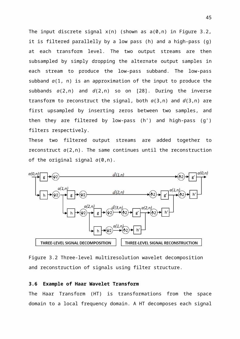
Figure 5.4 Baby image after wavelet decomposition two levels

The results obtained above are derived from the application of 2D haar wavelet transform.

The scaling and wavelet functions are separable. The summation is decomposed into two

stages. First step is along the x-axis and then the same operation is done along the y-axis.

Second step is along y-axis and then the same operation is done along the x-axis. A schematic

diagram is shown in Figure 5.4. The two dimensional signal is divided into four bands:

LL(left-top), HL(right-top), LH(left-bottom) and HH(right-bottom). The HL band, indicated

in Figure 5.3., is the variation along the x-axis while the LH band shows the y-axis variation.

Figure 5.3, 5.4, and 5.5 show the decomposition of a baby image. After selection of a

threshold, the hard thresholding is applied to the detail coefficients to get the compressed

image. The power is more compact in the LL band in the point of coding, we can spend more

bits on the low frequency band and less bit on the high frequency band or even set them to

zero.

Then we apply the inverse haar wavelet transform to the compressed image to get the

reconstructed image.

5.4 Image Compression Using Wavelet Neural Network

5.4.1 Procedure

45

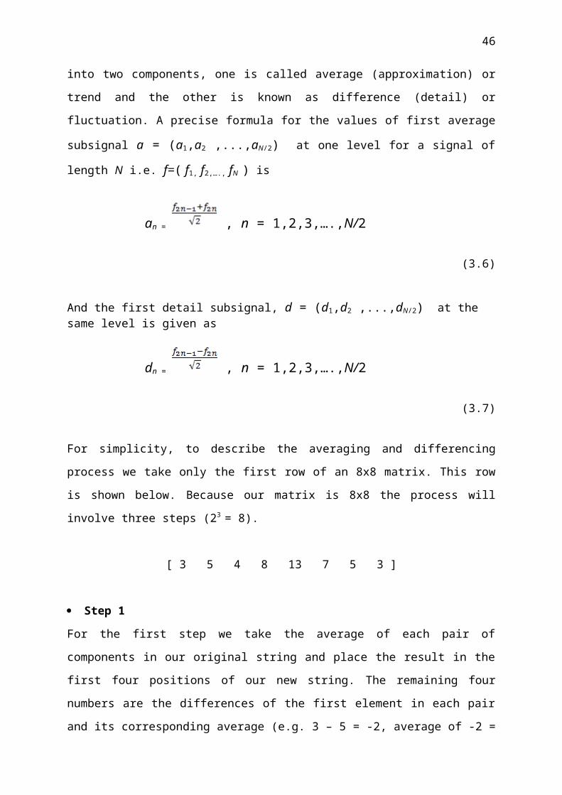
Our purpose is to use the combination of an artificial neural network and a mexican hat

wavelet network for compressing images. The network architecture is selected for the

problem of image compression. At first stage the image is represented in spatial domain. After

scaling and segmentation the input and output training data is formed. These data are used to

construct the structure of WNN. These are the selection the number of neurons in input,

hidden (wavelet) and output layers.. Both of input and output layers are fully connected to the

hidden layer. After selection of WNN structure the back propagation algorithm is used to

adjust the weights of WNN.

As mentioned before, the wavelet networks present certain architecture proximity with the

neural networks. The main similarity is that both networks calculate a linear combination of

non linear functions to adjust parameters. These functions depend on adjustable parameters

(dilations and translations). But the essential difference between them results from the nature

of the transfer functions used by the hidden cells.

5.4.2 Method Principle

In order to compress the image, first, we will segment it in a set of m blocks I by I pixels.

These blocks are used as inputs for the wavelet network. A three layer feed-forward neural

network is used: an input layer with m neurons with I2 block pixels, an output layer with m

neurons and a hidden layer with k number of neurons are used The value of k must be smaller

than m. It is affecting the number wavelet functions used. The WNN is trained in order to

reproduce the signals in the output that is given to input. We denote the input block by X=(x1,

….. xm) and the output of the network by Y=(y1,…..., ym). At the end of the training we aim

having Y=X for every block presented to the network is shown in Figure 5.5.

46

Figure 5.5 Representation of training stage.

5.4.3 Training algorithm

The WNN that includes input, hidden (wavelet) and output layers is used to design

compression system. Wavelet networks are designed through training using input/output

pairs. During training, the weights, dilations and translations parameters are iteratively

adjusted to minimize the mean square error which is called the network performance function.

A quadratic cost function is used to measure the error. Training aims to minimize the empiric

cost.

5.4.4 Algorithm

1. Divide the original image into 4x4 pixel blocks and reshaping each one into 16x1 column

vector.

2. Arranging all column vectors into a matrix of 16x4096.

3. Let the target matrix be equal to the matrix in step 2.

4. Choosing a suitable training algorithm, and defining the training parameters: the number of

iterations, the number of hidden neurons and the initial conditions;

5. Simulate the WNN by taking the two matrices of inputs and targets.

6. Obtain the output matrices of the hidden layer and the output layer.

7. Post-process them to obtain the compressed image, and the reconstructed image

respectively.

5.5 The Simulation Results

47

In Figure 5.6, the original and reconstructed images of Lena using Neural Network, Haar

Wavelet Transform and Wavelet Network (Mexican Hat Wavelet) are given with compression

ratio 25%. The training of NN and WNN systems has been performed using 5000 and 100

epochs, respectively.

(a) Original image of Lena.

(b) Reconstruction image of Lena using Haar Wavelet.

(c) Reconstruction image of Lena using Neural Network.

(d) Reconstruction image of Lena using Wavelet Network.

Original image reconstructed image

Original image reconstructed image(a) (b)

Original image reconstructed imageOriginal image reconstructed image (c) (d)

Figure 5.6 Lena images with compression ratio 25% [38].

In Figure 5.7, the original and reconstructed images of Lena using Neural Network, Haar

Wavelet Transform and Wavelet Network (Mexican Hat Wavelet) are given with compression

ratio 50%. The training of NN and WNN systems has been performed using 5000 and 100

epochs, respectively.

48

(a) Original image of Lena.

(b) Reconstruction image of Lena using Haar Wavelet.

(c) Reconstruction image of Lena using Neural Network.

(d) Reconstruction image of Lena using Wavelet Network.

Original image reconstructed image

Original image reconstructed image(a) (b)

Original image reconstructed imageOriginal image reconstructed image

(c) (d)

Figure 5.7 Lena images with compression ratio 50 % [38].

In Figure 5.8, the original and reconstructed images of Lena using Neural Network, Haar

Wavelet Transform and Wavelet Network (Mexican Hat Wavelet) are given with compression

ratio 75%. The training of NN and WNN systems has been performed using 5000 and 100

epochs, respectively.

(a) Original image of Lena.

(b) Reconstruction image of Lena using Haar Wavelet.

(c) Reconstruction image of Lena using Neural Network.

(d) Reconstruction image of Lena using Wavelet Network.

49

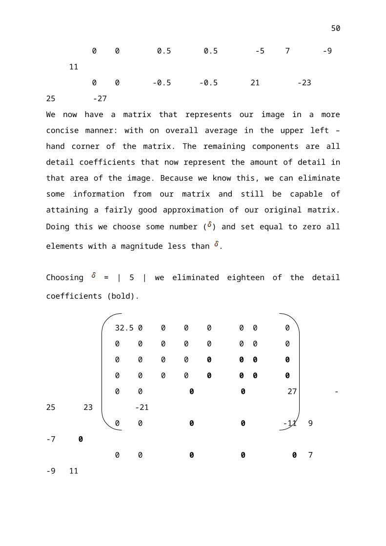
Original image reconstructed image

Original image reconstructed image(a) (b)

Original image reconstructed imageOriginal image reconstructed image (c) (d)

Figure 5.8 Lena images with compression ratio 75 % [38].

In Figure 5.9, the original and reconstructed images of Lena using Neural Network, Haar

Wavelet Transform and Wavelet Network (Mexican Hat Wavelet) are given with compression

ratio 87.50%. The training of NN and WNN systems has been performed using 5000 and 100

epochs, respectively.

(a) Original image of Lena.

(b) Reconstruction image of Lena using Haar Wavelet.

(c) Reconstruction image of Lena using Neural Network.

(d) Reconstruction image of Lena using Wavelet Network.

50

Original image reconstructed image

Original image reconstructed image(a) (b)

Original image reconstructed image

Original image reconstructed image

(c) (d)

Figure 5.9 Lena images with compression ratio 87.50 % [38].

In Figure 5.10, the original and reconstructed images of Peppers using Neural Network, Haar

Wavelet Transform and Wavelet Network (Mexican Hat Wavelet) are given with compression

ratio 25%. The training of NN and WNN systems has been performed using 5000 and 100

epochs, respectively.

(a) Original image of Peppers.

(b) Reconstruction image of Peppers using Haar Wavelet.

(c) Reconstruction image of Peppers using Neural Network.

(d) Reconstruction image of Peppers using Wavelet Network.

51

Original image reconstructed image

(a) (b)

Original image reconstructed imageOriginal image reconstructed image

(c) (d)

Figure 5.10 Peppers images with compression ratio 25 %.

In Figure 5.11, the original and reconstructed images of Peppers using Neural Network, Haar

Wavelet Transform and Wavelet Network (Mexican Hat Wavelet) are given with compression

ratio 50%. The training of NN and WNN systems has been performed using 5000 and 100

epochs, respectively.

(a) Original image of Peppers.

(b) Reconstruction image of Peppers using Haar Wavelet.

(c) Reconstruction image of Peppers using Neural Network.

(d) Reconstruction image of Peppers using Wavelet Network.

52

Original image reconstructed image

Original image reconstructed imageOriginal image reconstructed image (a) (b)

Original image reconstructed imageOriginal image reconstructed image

(c) (d)

Figure 5.11 Peppers images with compression ratio 50 %.

In Figure 5.12, the original and reconstructed images of Peppers using Neural Network, Haar

Wavelet Transform and Wavelet Network (Mexican Hat Wavelet) are given with compression

ratio 75%. The training of NN and WNN systems has been performed using 5000 and 100

epochs, respectively.

(a) Original image of Peppers.

(b) Reconstruction image of Peppers using Haar Wavelet.

(c) Reconstruction image of Peppers using Neural Network.

(d) Reconstruction image of Peppers using Wavelet Network.

53

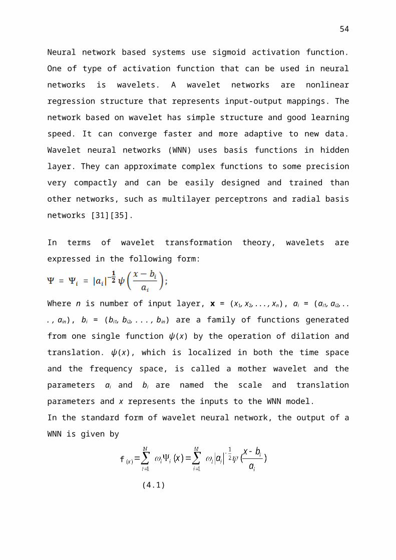
Original image reconstructed image

Original image reconstructed image(a) (b)

Original image reconstructed image

Original image reconstructed image

(c) (d)

Figure 5.12 Peppers images with compression ratio 75 %.

In Figure 5.13, the original and reconstructed images of Peppers using Neural Network, Haar

Wavelet Transform and Wavelet Network (Mexican Hat Wavelet) are given with compression

ratio 87.50%. The training of NN and WNN systems has been performed using 5000 and 100

epochs, respectively.

(a) Original image of Peppers.

(b) Reconstruction image of Peppers using Haar Wavelet.

(c) Reconstruction image of Peppers using Neural Network.

(d) Reconstruction image of Peppers using Wavelet Network.

54

Original image reconstructed image

Original image reconstructed image (a) (b)

Original image reconstructed image

Original image reconstructed image

(c) (d)

Figure 5.13 Peppers images with compression ratio 87.50 %.

In Figure 5.14, the original and reconstructed images of Baby using Neural Network, Haar

Wavelet Transform and Wavelet Network (Mexican Hat Wavelet) are given with compression

ratio 25%. The training of NN and WNN systems has been performed using 5000 and 100

epochs, respectively.

(a) Original image of Baby.

(b) Reconstruction image of Baby using Haar Wavelet.

(c) Reconstruction image of Baby using Neural Network.

(d) Reconstruction image of Baby using Wavelet Network.

55

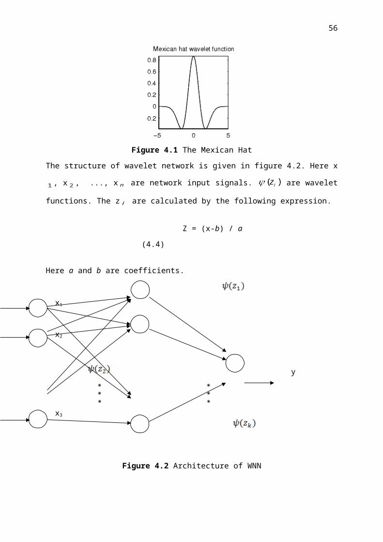
Original image reconstructed image

Original image reconstructed image (a) (b)

Original image reconstructed imageOriginal image reconstructed image

(c) (d)

Figure 5.14 Baby images with compression ratio 25 %.

In Figure 5.15, the original and reconstructed images of Baby using Neural Network, Haar

Wavelet Transform and Wavelet Network (Mexican Hat Wavelet) are given with compression

ratio 50%. The training of NN and WNN systems has been performed using 5000 and 100

epochs, respectively.

(a) Original image of Baby.

(b) Reconstruction image of Baby using Haar Wavelet.

(c) Reconstruction image of Baby using Neural Network.

(d) Reconstruction image of Baby using Wavelet Network.

56

Original image reconstructed imageOriginal image reconstructed image (a) (b)

Original image reconstructed imageOriginal image reconstructed image

(c) (d)

Figure 5.15 Baby images with compression ratio 50 %.

In Figure 5.16, the original and reconstructed images of Baby using Neural Network, Haar

Wavelet Transform and Wavelet Network (Mexican Hat Wavelet) are given with compression

ratio 75%. The training of NN and WNN systems has been performed using 5000 and 100

epochs, respectively.

(a) Original image of Baby.

(b) Reconstruction image of Baby using Haar Wavelet.

(c) Reconstruction image of Baby using Neural Network.

(d) Reconstruction image of Baby using Wavelet Network.

57

Original image reconstructed imageOriginal image reconstructed image (a) (b)

Original image reconstructed image

Original image reconstructed image (c) (d)

Figure 5.16 Baby images with compression ratio 75 %.

In Figure 5.17, the original and reconstructed images of Baby using Neural Network, Haar

Wavelet Transform and Wavelet Network (Mexican Hat Wavelet) are given with compression

ratio 87.50%. The training of NN and WNN systems has been performed using 5000 and 100

epochs, respectively.

(a) Original image of Baby.

(b) Reconstruction image of Baby using Haar Wavelet.

(c) Reconstruction image of Baby using Neural Network.

(d) Reconstruction image of Baby using Wavelet Network.

58

Original image reconstructed imageOriginal image reconstructed image (a) (b)

Original image reconstructed imageOriginal image reconstructed image (c) (d)

Figure 5.17 Baby images with compression ratio 87.50 %

.5.6 Impementation and Results

The tests are made on the three images taken from the Matlab library, called: Lena, Peppers

and Baby. The performances of image compression are based on the two following criteria:

the compression rate CR and the quality of the reconstruction image PSNR. The values of the

CR, MSE, PSNR, B/P, Size of Compression image and the computational Time of images for

each technique are presented below.

Table 5.1 The results for Lena images using Neural Networks.

CR MSE PSNR (dB) Bits/pixel Size by kbyte

Computational Time

25% 0.3807 52.3243 5.9947 47.9578 0.48 sec

50% 0.5224 50.9508 3.7117 31.6934 0.45 sec

75% 0.6685 49.8795 1.7573 15.4587 0.44 sec

87.5% 0.8942 48.6164 0.8480 7.7584 0.39 sec

59

Table 5.2 The results for Lena images using Haar Wavelet Transform.

CR MSE PSNR (dB) Bits/pixel Size by kbyte

Computational Time

25% 0.1108 57.6854 5.7426 46.9412 0.72 sec

50% 0.1942 55.2483 3.9254 31.4028 0.60 sec

75% 0.3762 52.3766 1.7818 15.2543 0.59 sec

87.5% 0.6297 50.1395 1.2207 8.7655 0.56 sec

Table 5.3 The results for Lena images using Mexican Hat Wavelet Networks.

CR MSE PSNR (dB) Bits/pixel Size by kbyte

Computational Time

25% 0.0193 65.2752 6.1047 48.7218 0.63 sec

50% 0.0754 59.3571 3.5176 29.4625 0.57 sec

75% 0.1154 57.5087 1.6564 15.304 0.51 sec

87.5% 0.1876 55.3985 0.9394 7.9323 0.45 sec

Table 5.4 The results for Peppers images using Neural Networks.

CR MSE PSNR (dB) Bits/pixel Size by kbyte

Computational Time

25% 0.4146 51.9545 5.9967 47.9739 0.54 sec

50% 0.2353 54.4146 3.5966 29.7728 0.48 sec

75% 0.3719 52.4265 2.1168 16.9343 0.44 sec

87.5% 0.8607 48.7818 0.9099 7.2798 0.42 sec

Table 5.5 The results for Peppers images using Haar Wavelet Transform.

CR MSE PSNR (dB) Bits/pixel Size by kbyte

Computational Time

25% 0.1529 56.2867 5.62 bpp 47.99 kbyte 0.73 sec

50% 0.2276 54.5591 3.78 bpp 31.24 kbyte 0.69 sec

75% 0.2628 53.9345 2.02 bpp 16.19 kbyte 0.63 sec

87.5% 0.7148 49.5890 1.04 bpp 8.04 kbyte 0.63 sec

Table 5.6 The results for Peppers images using Mexican Hat Wavelet Networks.

60

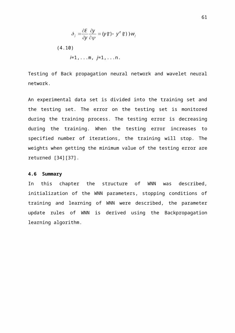
CR MSE PSNR (dB) Bits/pixel Size by kbyte

Computational Time

25% 0.0313 63.1754 5.6145 47.7723 0.59 sec

50% 0.0552 60.7114 3.8455 31.3455 0.56 sec

75% 0.0897 58.6029 1.7344 15.2463 0.55 sec

87.5% 0.2343 54.4331 0.8544 7.6434 0.54 sec

Table 5.7 The results for Baby images using Neural Networks.

CR MSE PSNR (dB) Bits/pixel Size by kbyte

Computational Time

25% 0.3214 53.1698 5.9216 47.3732 0.49 sec

50% 0.4274 51.8225 3.8705 30.9641 0.47 sec

75% 0.5714 50.5614 2.2752 18.2018 0.46 sec

87.5% 2.9457 43.4389 1.0783 8.6261 0.39sec

Table 5.8 The results for Baby images using Haar Wavelet Transform.

CR MSE PSNR (dB) Bits/pixel Size by kbyte

Computational Time

25% 0.1246 57.1756 5.8228 46.582 0.75 sec

50% 0.2463 54.2162 3.9737 31.7899 0.66 sec

75% 0.3141 53.1601 1.8489 14.7909 0.68 sec

87.5% 0.4586 51.5165 1.0118 9.7439 0.62 sec

Table 5.9 The results for Baby images using Mexican Hat Wavelet Networks.

CR MSE PSNR (dB) Bits/pixel Size by kbyte

Computational Time

25% 0.0375 62.3905 5.3237 47.1204 0.61 sec

50% 0.0786 59.1766 3.5433 30.5654 0.58 sec

75% 0.0874 58.7157 1.3207 15.4534 0.54 sec

87.5% 0.1198 57.3462 0.9764 7.4354 0.53 sec

5.6.1 Comparison Using PSNR Values

61

All three tests are made for different compression ratio (25 %, 50 %, 75 % and 87.5 %).

- For Lena Images

Table 5.10 The values of MSE, PSNR and compression rate for Lena images.

Techniques MSE PSNR (dB) Compression Rate

Neural Networks

0.3807 52.3243 25%0.5224 50.9508 50%0.6685 49.8795 75%0.8942 48.6164 87.5%

Haar Wavelet Transform

0.1108 57.6854 25%0.1942 55.2483 50%0.3762 52.3766 75%0.6297 50.1395 87.5%

Wavelet Neural Networks

0.0193 65.2752 25%0.0754 59.3571 50%0.1154 57.5087 75%0.1876 55.3985 87.5%

- For Peppers Images

Table 5.11 The values of MSE, PSNR and compression rate for Peppers images.

Techniques MSE PSNR (dB) Compression Rate

Neural Networks

0.4146 51.9545 25%0.2353 54.4146 50%0.3719 52.4265 75%0.8607 48.7818 87.5%

Haar Wavelet Transform

0.1529 56.2867 25%0.2276 54.5591 50%0.2628 53.9345 75%0.7148 49.5890 87.5%

Wavelet Neural Networks

0.0313 63.1754 25%0.0552 60.7114 50%0.0897 58.6029 75%0.2343 54.4331 87.5%

- For Baby Images

62

Table 5.12 The values of MSE, PSNR and compression rate for Baby images.

Techniques MSE PSNR (dB) Compression Rate

Neural Networks

0.3214 53.1698 25%0.4274 51.8225 50%0.5714 50.5614 75%2.9457 43.4389 87.5%

Haar Wavelet Transform

0.1246 57.1756 25%0.2463 54.2162 50%0.3141 53.1601 75%0.4586 51.5165 87.5%

Wavelet Neural Networks

0.0375 62.3905 25%0.0786 59.1766 50%0.0874 58.7157 75%0.1198 57.3462 87.5%

In the image compression the quality of the reconstructed image and compression ratio are

important factors. In this chapter, the PSNR results of used techniques are compared. The

analysis of the simulation results shown that the WNN that uses Mexican hat wavelet has

obtained high performances compared to classical neural network and haar wavelet transform.

The results shown that the haar wavelet transform approach provides more efficiency

compared with the neural networks, but neural networks take less time than wavelet

transform, when the same compression ratio is used for each technique.

5.6.2 Comparison of Computational Time of Used Techniques

During compression of the results the computer with (2.3 GHz.) is used.

Table 5.13 The computational time and compression rate for Lena, Peppers and Baby images.

Techniques Images Computational Time Compression rate

Neural Networks

For lena

0.48 sec 25%0.45 sec 50%0.44 sec 75%0.39 sec 87.5%

Haar Wavelet Transform

0.72 sec 25%0.60 sec 50%0.59 sec 75%0.56 sec 87.5%

Wavelet (Mexican Hat)

For lena 0.63 sec 25%0.57 sec 50%

63

Networks0.51 sec 75%0.45 sec 87.5%

Neural Networks

For Peppers

0.54 sec 25%0.48 sec 50%0.44 sec 75%0.42 sec 87.5%

Haar Wavelet Transform

0.73 sec 25%0.69 sec 50% 0.63 sec 75%0.63 sec 87.5%

Wavelet (Mexican Hat)

Networks

0.59 sec 25%0.56 sec 50%0.55 sec 75%0.54 sec 87.5%

Neural Networks

For Baby

0.49 sec 25%0.47 sec 50% 0.46 sec 75%0.39sec 87.5%

Haar Wavelet Transform

0.75 sec 25%0.66 sec 50% 0.68 sec 75%0.62 sec 87.5%

Wavelet (Mexican Hat)

Networks

0.61 sec 25%0.58 sec 50%0.54 sec 75%0.53 sec 87.5%

5.7 Summary

In this chapter, the image compression techniques using Neural Network, Haar Wavelet

Transform and (Mexican Hat) Wavelet Network were described. The used techniques are

applied to different images and all the reconstructed images are analysed using the

comparison criteria. The results of each technique, using PSNR, and computational time are

presented.

6. CONCLUSIONS

64

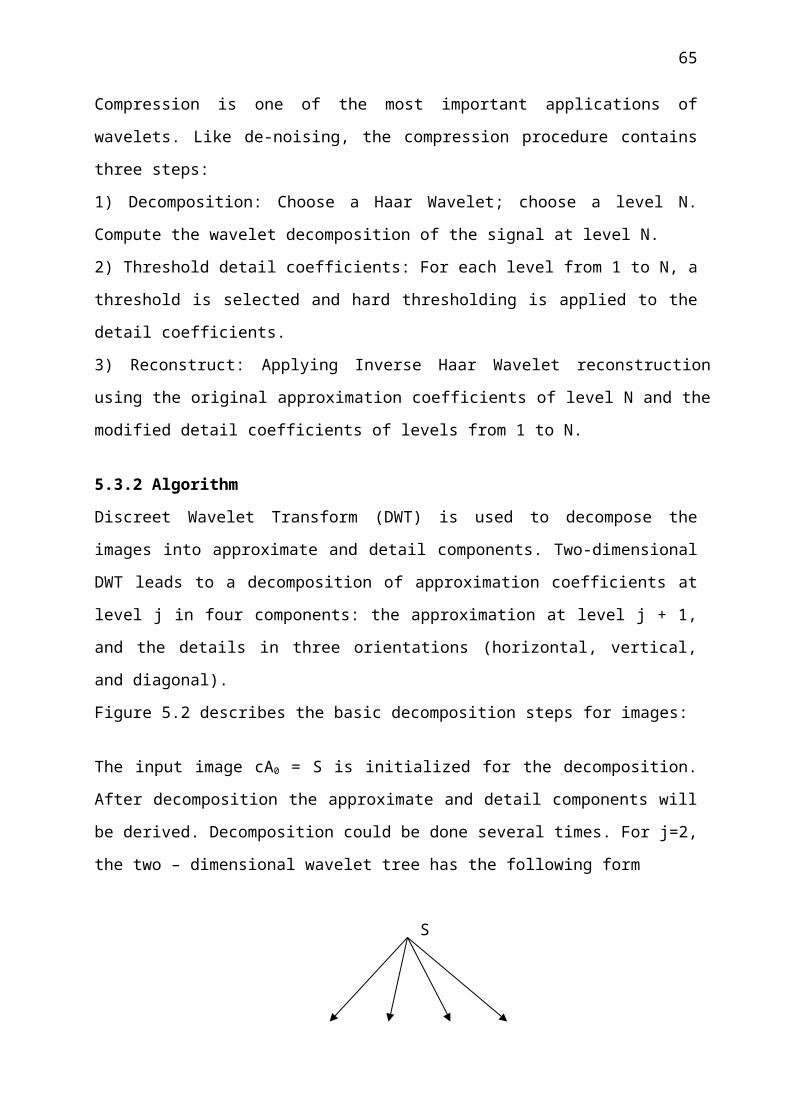
The storage and transmission of huge mass of information is one of the important problems in

computer science. To solve this problem different data compression techniques have been

designed. In this thesis the design of image compressing systems using Neural Networks,

Wavelets and Wavelet Neural Networks have been considered.

The analysis of image compression techniques has been performed. The state of usage of

Neural and Wavelet techniques for image compression is given.

The design principle of NN based on image compression system is given. The structure of

neural networks is selected and the learning of neural network based image compression

system using back-propagation algorithm was described.

The properties of wavelet and discrete wavelet transform subsignal encoding are described.

Using discrete wavelet transform, the multiresolution analysis of wavelet, the development of

image compression system is described.

The structure of Wavelet Neural Network for image compression is designed. Initialization of

the WNN parameters, its learning algorithm and stopping conditions for training are

described, using the back propagation algorithm. The parameter update rules of WNN are

presented.

The design of image compression systems using Neural Network, Wavelet Network and

Wavelet Transform are carried out. The steps of image compression using these techniques

have been performed. The comparison results of each technique for different image examples

are presented using different values of compression rates. Comparative results of used

techniques are based on peak signal-to-noise ratio (PSNR), mean square error (MSE),

computational time and the quality of the reconstructed images. The obtained simulation

results demonstrate that when compression rate is increased the image compression system

based on WNN gives better results.

Simulation of the image compression systems based on NN, wavelet and WNN have been

carried out using Matlab program and PC.

REFERENCES

65

[1] David Jeff Jackson and Sidney Jwl Hannah, “Comparative Analysis of image compression

technique”, twenty fifth edition southeastern symposiums on 9th march 1993, pp. 513-517.

[2] Ronald A.DeVore, Bjorn Jawerth, and Bradley J.Lucier, “Image Compression Through

Wavelet Transforms Coding” IEEE transactions on information theory, Vol. 38. NO. 2,

March 1992, pp. 719-746.

[3] Sachin Dhawan, “A Review of Image Compression and Comparison of its Algorithms”,

International Journal of Electronics & Communication Technology, Vol. 2, Issue 1, March

2011, pp. 22-26.

[4] Rahib H. Abiyev ,”Algorithm”, Near East University (NEU) - Nicosia, 2006.

[5] Jagadish H. Pujar and Lohit M. Kadlaskar “A new lossless method of image compression

and decompression using Huffman coding techniques”, Journal of Theoretical and Applied

Information Technology, pp. 18-23, 2010.

[6] “Image Compression”, http://en.wikipedia.org/wiki/image_compression, 23, March 2012.

[7] Ian Witten, Radford Neal, and John Cleary, "Arithmetic Coding for Data Compression",

Communications of the ACM, June 1987, Vol. 30, No. 6, pp. 520-540.

[8] yun Q. Shi Huifang Sun, “Image and Video Compression for Multimedia Engineering“,

Second Edition, New Jersey Institute of Technology Newark, USA, 2008 by Taylor, &

Francis Group, LLC.

[9] Terry Welch, "A Technique for High-Performance Data Compression", IEEE Computer,

June 1984, pp. 8-19.

[10] N Nopparat Pantsaena, M. Sangworasil, C. Nantajiwakornchai and T. Phanprasit, "Image

coding using vector quantization” The Research Center for Communication and Information

Technology.

[11] “Quantization”, http://www.debugmode.com/imagecmp/quantize.htm, 24, March 2012.

[12] Deng, Li; Douglas O'Shaughnessy (2003). Speech processing: a dynamic and

optimization-oriented approach. Marcel Dekker. pp. 41–48.

66

[13] Wavelets - Jöran Bergh, Fredrik Ekstedt, Martin Lindberg, 1 Oca 1999.

[14] Neural Networks: “A Comprehensive Foundation”, Second Edition. Simon Haykin.

Prentice Hall, 1999, Ontario, Canada.

[15] Wilford Gillespie “Still image compression using Neural Networks" Utah State Univer-

sity, Logan, UT, 1998.

.[16] Rupinder Singh ana Jarnail Singh, “Edge Preserving Image Compression Technique

using Feed Forward Neural Network”, International Journal of Computer Science and

Technology, Vol. 2, Issue 1, March 2011, pp. 137-138.

[17] Narayanan Sreekumar and Dr. S.Santhosh Baboo, “Neural Network based Complex

Image Compression using Modified Levenberg-Marquardt method for Learning”

International Journal of Computer Science and Technology, Vol. 2 Issue 2, June 2011, pp.

349-354.

[18] Weiwei Xiao, Haiyan Liu, “Using Wavelet Networks in Image Compression“, Seventh

International Conference on Natural Computation, pp. 700-704, 2011, Beijing, China.

[19] O. Jemai, C. Ben Amar “A new scheme of Image Compression using wavelet networks”,

Research Group on Intelligent Machines, 2005, Tunisia.

[20] Tracy Denk, Keshab K. Parhi, and Wadimir Cherkassky, “Combining Neural Networks

and the Wavelet Transform for image compression”, IEEE International Conference on

Acoustics, pp. 637-640, 1993.

[21] “Supervised Learning”, http://neurondotnet.freehostia.com/manual/types.html, 4, Nissan

2012.

[22] “Unsupervised Learning”, http://irrigation.rid.go.th/rid15/ppn/Knowledge/Artificial

Neuron Networks Technology Neural Networks Components.htm, 4, Nissan 2012.

[23] Yahya M. Masalmah “Image Compression Using Neural Networks”, University of Pu-

erto Rico, 2003.

[24] “Wavelet Transform”, http://www.amara.com/IEEEwave/IEEEwavelet.html, 17, Nissan

2012.

67

[25] Kamrul Hasan Talukder and Koichi Harada, “Haar Wavelet Based Approach for Image

Compression and Quality Assessment of Compressed Image”, International Journal of

Applied Mathematics, Advance online publication: 1 February 2007.

[26] Jung-Hua Wang and Mer-Jiang Gou, “Image Compression Using Wavelet Transform

and Self-development Neural Network”, pp. 4104-4108, 1998, Taiwan.

[27] Sonja Grgic and Branka Zovko , “Performance Analysis of Image Compression Using

Wavelets” IEEE Transactions on Industrial Electronics, Vol. 48, No. 3, JUNE 2001, pp. 682 –

695.

[28] Vipula Singh, Navin Rajpal and K. Shrikanta .Murthy, “Neuro-Wavelet Based Approach

for Image Compression”. Computer Graphics, Imaging and Visualisation (CGIV 2007)

[29] Zhang,Q. and Benveniste, “A Wavelet Networks”, IEEE Transactions on Neural

Networks, Vol 3,No. 6, pp. 889-898, 1992.

[30] Szu,H., Telfer, B. and Garcia, J., “Wavelet Transform and Wavelet Networks for

Composition and Recognition, Neural Networks”, Vol. 9, pp. 695-708, 1996.

[31] Wajdi Bellil, Chokri Ben Amar, and Adel M. Alimi, “Comparison between Beta

Wavelets Neural Networks, RBF Neural Networks and Polynomial Approximation for 1D,

2D Functions Approximation”, Poceedings of World Academy of Science, Engineering and

Technology vol. 13, May 2006, pp. 102 107.

[32] Yacine OUSSAR and Gérard DREYFUS, “Initialization by Selection for Wavelet Net-

work Training”, Neurocomputing vol. 34, pp. 131-143 (2000).

[33] Xian-Bin Wen, Hua Zhang and Fa-Yu Wang, “A Wavelet Neural Network for SAR Im-

age Segmentation”, pp. 7510 – 7515, 2009.

[34] Rahib Abiyev, Mehmet Ali Salahli, Development of Wavelet Neural Network based

Controller. 3rd FAE International Symposium ”Creating the Future”. Lefke, TRNC, Turkey,

November 25-26, 2004.

[35] Rahib Abiyev, Mehmet Ali Salahli, Controller Based on Wavelet Neural network. 4-th

International Symposium on Intelligent Manufacturing Systems. IMS’2004, Sakarya,

September 6-8, 2004.

68

[36] Rahib H.Abiyev. Fuzzy Wavelet Neural Network Based on Fuzzy Clustering and

Gradient Techniques for Time Series Prediction. Neural Computing & Applications, Vol. 20,

No. 2, pp. 249-259, 2011.

[37] Rahib H.Abiyev and Okyay Kaynak, “Identification and Control of Dynamic Plants Us-

ing Fuzzy Wavelet Neural Networks”, IEEE IEEE Transactions on Industrial Electronics,

Vol. 55, No. 8, August 2008, pp. 3133 - 3140.

[38] "Lena Image",h ttp://www.svgopen.org/2007/papers/NovelRenderingOrderSVGVector iz

ation/index.html 4, Nissan 2012.

Appendix 1.1 Neural Networks

clear;I = imread('photo/peppers.jpg');I=imresize(I,[256 256]);

69

I=rgb2gray(I);[row,col]=size(I);in1=I;r=4;c=4;hav=double(in1)/255; in2=blkM2vc(hav,[r c]); in3=in2;in4=in3;[a b]=size(in4);functions={'purelin','logsig','purelin'};% [hidden ,hidden , output] net=newff(minmax(in3),[20 1 a],functions,'traingdx');%net.trainparam.show=5;

net.trainparam.epochs=1000;net.trainparam.goal=1e-5;net.trainparam.lr=0.15;net.trainparam.mc=0.1;%0.09 er=336 [net_s,tr]=train(net,in3,in4);a=sim(net_s,in3);fr=vc2blkM(a,r,c,256);%fr=vec2block(a,r);rec_photo=fr;fr=fr*255;az=uint8(fr);figure(20);subplot(1,2,1)imshow(I); xlabel('Original image');subplot(1,2,2)imshow(az); xlabel('reconstructed image');im_comp;

Appendix 1.2 Haar Wavelet Transform

clear all;closeclcthr=0.20;a=imread('photo/lena.jpg'); a=rgb2gray(a);I=a;a=double(a)./255;a1=imresize(a,[256 256]);image=a1; [lll mmm]=size(a1); if(mmm~=lll), error('the image must be square'); end stage=0; while(lll~=1) lll=floor(lll/2); stage=stage+1;end

70

levels=input('please enter the levels of wavelet compression = '); levels=levels-1; for n=stage:-1:stage-levels % it was 1 clc %to construct matrix horizontally m=2^n; m_2=m/2; m_22=m/4; a=0.5*eye(m_2); b=eye(m_2); c=-1*eye(m_2); d(1:2:m,:)=a; d(2:2:m,:)=a; e(1:2:m,:)=b; e(2:2:m,:)=c; w=[d e]; a=[]; b=[]; c=[]; d=[]; e=[]; %to apply transform x=image(1:m,1:m)*w; w=[];

% construct vertical matrix a=0.5*eye(m_2); b=eye(m_2); c=-1*eye(m_2); d(:,1:2:m)=a(:,1:m_2); d(:,2:2:m)=a(:,1:m_2); e(:,1:2:m)=b(:,1:m_2); e(:,2:2:m)=c(:,1:m_2); wv=[d ; e]; o=x(1:m,1:m_2); o2=x(1:m,m_2+1:m); y=wv*o; wv=[]; y1=[y o2]; %imshow(x); image(1:m,1:m)=y1; figure(2) imshow(image) a=[]; b=[]; c=[]; d=[]; e=[]; wv=[]; y1=[]; endcom_img=image;Appendix 1.3 Mexican Hat Wavelet Networks

clear;scale1=256;I = imread('photo/lena.jpg');I=imresize(I,[scale1 scale1]);I=rgb2gray(I);imshow(I);[row,col]=size(I);in1=I;

71

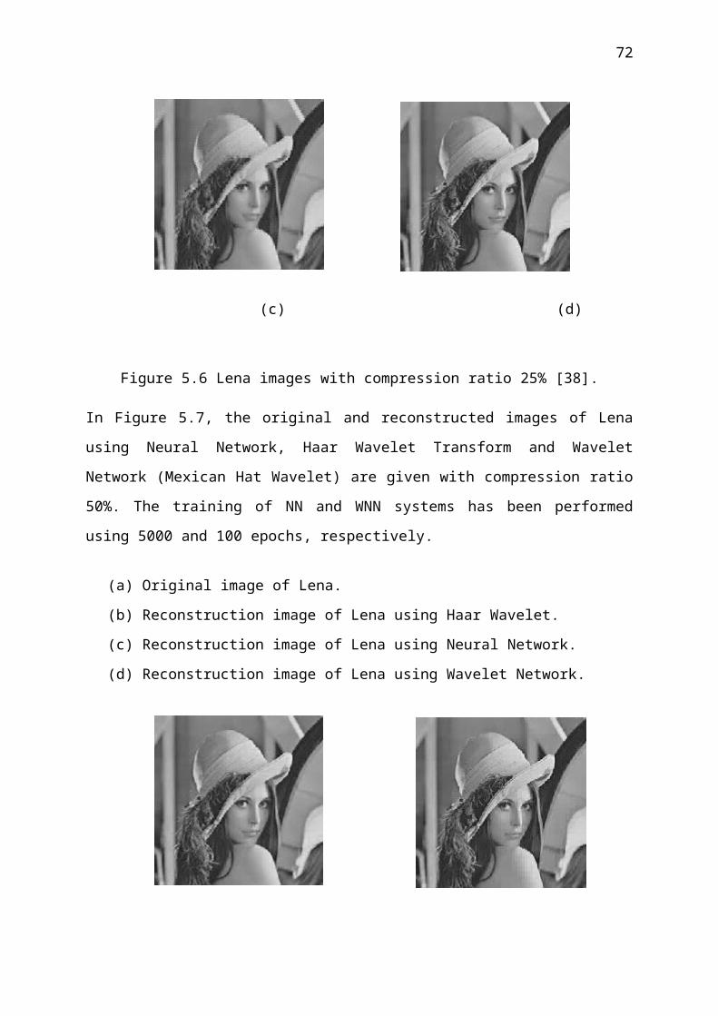
r=4;c=4;hav=double(in1)/255;in2=blkM2vc(hav,[r c]) in3=in2';[r1 c1]=size(in2) P=1; m=r1%number of input node n=3%number of hidden node N=m%number of ouptut nodeW=0.002*rand(N,n);WW=0.002*rand(n,m)a=ones(1,n)for j=1:nb(j)=j*P/n;endregim=1; for j=1:3 sumer=0; for i=1:c1 x(P,:)=in2(:,i); d=x; [W,WW,a,b,u,y,error,phi]=WnnMH(regim,P,m,n,N,x,d,W,WW,a,b); [yt(i,:)]=[y]; [ph(i,:)]=[phi]; sumer=sumer+error; end sprintf('I-th epoch= %f Sum of Errors=%f',j,sumer)end ytwnn=yt'; comp_image=ph'; fr=vc2blkM(ytwnn,r,c,scale1);rec_photo=fr;fr=fr*255;az=uint8(fr);figure(20);subplot(1,2,1)imshow(I); xlabel('Original image');subplot(1,2,2)imshow(az); xlabel('reconstructed image');psnr;

72