y. okabe and t. yamane - cambridge university press...y. okabe and t. yamane nagoya math. j. vol....

Y. Okabe and T. YamaneNagoya Math. J.Vol. 152 (1998), 175-201

THE THEORY OF KM2O-LANGEVIN EQUATIONS ANDITS APPLICATIONS TO DATA ANALYSIS (III):

DETERMINISTIC ANALYSIS

YASUNORI OKABE AND TOSHIYUKI YAMANE

Abstract. A technique is given for detecting deterministic dynamics in timeseries. Some stochastic difference equations, called KM^O-Langevin equations,are extracted directly from given data. We can find deterministic dynamicsin time series by evaluating the magnitude of innovation part of the KM2O-Langevin equations. We can further find chaotic dynamics in time series bypredicting it from the viewpoint of the theory of KlVhO-Langevin equations.

We apply our method to the data of measles and chicken pox, which are alsotreated by G.Sugihara and R.M.May in [1]. The result of numerical experimentsindicates that there seem to exist some deterministic dynamics in both timeseries. It also suggests, however, that the data of measles seems to be chaoticwhile that of chicken pox not, which corresponds to the result of G.Sugiharaand R.M.May.

§1. Introduction

There are a lot of systems in the world, whose behavior as a whole isnever understandable if we only view their components separately. Suchsystems, called complex systems, arise from a variety of origins of com-plexity such as stochastic structure, deterministic chaos and so on. Thisfeature of complex systems has the result that a priori parametric statisticalmodels (e.g. ARMA model, linear regression model) may fail to catch theunderlying structure arising from the complex systems which lies behindthe data.

Therefore, we must check the validity of the preconditions that is as-sumed before data analysis. We call such an approach toward data analysisa qualitative approach in contrast to quantitative approaches such as para-metric statistical models. One of the authors has presented a precondition-

Received July 7, 1997.This research was partially supported by Grant-in-Aid for Science Research (B)

No. 07459007 and Grant-in-Aid for Exploratory Research No. 08874007, the Ministryof Education, Science, Sports and Culture, Japan and by Promotion Work for CreativeSoftware, Information-Technology Promotion Agency, Japan.

175

https://www.cambridge.org/core/terms. https://doi.org/10.1017/S002776300000684XDownloaded from https://www.cambridge.org/core. IP address: 54.39.106.173, on 28 Jun 2020 at 13:54:36, subject to the Cambridge Core terms of use, available at

https://www.cambridge.org/core/terms

https://doi.org/10.1017/S002776300000684X

https://www.cambridge.org/core

176 Y. OKABE AND T. YAMANE

free method of qualitative approach to time series based on the theory ofKM2O-Langevin equations [3], [4], [5], [6], [7], [8], [9].

The theory of KM^O-Langevin equations is a new method of time se-ries analysis that originates from the study of the fluctuation-dissipationtheorem which is thought to be one of the principles of nonequilibrium sta-tistical physics. The main feature of this theory is that it requires no priorinformation about data and does not define any parametric models beforedata analysis, but extracts explanatory models in the form of stochasticdifference equations directly from data.

The most fundamental qualitative property of this theory is stationarityof time series. Testing stationarity of given time series is possible usingTest(S), which is established in [4], We can go to the next step of analysisonly for data whose stationarity is assured by Test(S). Given two stationarytime series, we can discuss whether they are related to each other, or in otherwords, whether there exists some causality between them by using Test(CS)in [7].

The contents of this paper are the following. First, in section 2 andsection 3, we briefly review the theory of KM2θ-Langevin equations and itsapplication to causality analysis which is developed in [3],[6]. Secondly, insection 3, we give a definition of nonlinear causality and give a method ofchecking it based on the Bootstrap method [10]. The results described hereare the extension of [7]. Thirdly, in section 4, we give a method of checkingwhether there exist some deterministic dynamics in a stationary time seriesby applying Test(CS), which is called Test(D). The importance to checkdeterminism in time series is argued in [1], and we can give an answer tothis question using Test(D). Fourthly, in section 4, we give a method oftesting whether the underlying dynamics in time series are chaotic fromthe viewpoint of prediction analysis in [5], [8]. Finally, in section 5, inorder to make the analysis in [9] more precise, we apply our method tothe measles data and chickenpox data, which are thought to originate fromsome complex systems. It is reported in [1] that the measles data appearchaotic, while the chickenpox data show a seasonal cycle with additive noise.We wish to take up the more basic question of whether these time seriescan really be thought to come from deterministic dynamic systems beforea discussion of whether they are chaotic or not. The result of numericalexperiments indicates that there seem to exist some deterministic dynamicsin both time series. It also suggests, however, that the measles data seem



https://doi.org/10.1017/S002776300000684X


LANGEVIN EQUATIONS AND ITS APPLICATIONS 177

to be chaotic while the chickenpox data are not, which corresponds to the

result of [1],

The authors would like to express their gratitude to Mr. A. Kaneko for

his helpful support in computer experiments.

§2. A short review of the theory of KM^O-Langevin equations

2.1. KM2θ-Langevin equation

Let X = (X(n); \n\ < N) be any Revalued stochastic process on a

probability space (Ω, £?, P). We introduce the forward KM2 O-Langeυin fluc-

tuation flow v+ = (z/+(n);0 < n < N) associated with X by projecting

X(n) on the vector space M Q ~ 1 ( X ) which is spanned by {Xj(k)\ 0 < k <

n-l, l<j<d}:

(1) i/+(0)=X(0)

(2) i/+(n) = X ( n ) - P M n - i ( x ) X ( n ) (1 < n < N),

where Pwι-i,χ^ denotes for the projection operator to M Q ~ 1 ( X ) .

In the same way, we introduce the backward KM2 O-Langeυin fluctuation

flow i/_ = (v-{l)\ -N < i < 0) by

(3) M O )

(4) v.{ί) = X(i) - PMo+i{x)X(£), (~N<1< -1).

The forward and backward KM2θ-Langevin fluctuation flows are sometimes

called innovation processes of X.

We assume the following independence condition for X:

{{Xj(n); 0 < n < N - 1,1 < j < d) is

linearly independent in ^ 1

{Xj(-n); 0 < n < N - 1,1 < j < d} is

linearly independent in

Then, we can derive the stochastic difference equation that describes the

time evolution of X in the following way:

π - l

(6) X{±n) = - Σ Ί±(n, k)X(±k) - δ±(ή)X(0) + v±{±n)fc=l

(0 < n < N),



https://doi.org/10.1017/S002776300000684X



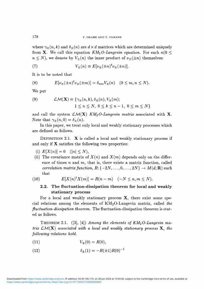
where 7±(n, k) and δ±(n) are d x d matrices which are determined uniquely

from X. We call this equation KM2 O-Langeυin equation. For each n(0 <

n < JV), we denote by V±{n) the inner product of ι/±(ήzn) themselves:

(7) V±(n) = E[v±{±n)t

V±(±n)].

It is to be noted that

(8) E[p±{±n)tv±{±m)) = δnmV±(n) (0 < m,n < N).

We put

(9) £M(X) = {7±(n, fc), «±(Ό, V±(m);

l < n < i V , 0 < Jk < n - 1, 0 < m < Λ Γ }

and call the system JCM(X.) KM2O-Langeυin matrix associated with X.

Note that 7±(ra,0) = S±(n).

In this paper, we treat only local and weakly stationary processes which

are defined as follows.

DEFINITION 2.1. X is called a local and weakly stationary process if

and only if X satisfies the following two properties:

(i) E[X(n)} = 0 (|n| < N),

(ii) The covariance matrix of X(n) and X(m) depends only on the differ-

ence of times n and ra, that is, there exists a matrix function, called

correlation matrix function, R: { —2ΛΓ,..., 0, . . . , 2iV} —> M(d\ R) such

that

(10) E[X(n)*X(m)] - R(n - m) {-N <n,m<N).

2.2. The fluctuation-dissipation theorem for local and weaklystationary process

For a local and weakly stationary process X, there exist some spe-

cial relations among the elements of KM^O-Langevin matrix, called the

fluctuation-dissipation theorem. The fluctuation-dissipation theorem is stat-

ed as follows.

THEOREM 2.1. ([3], [4]) Among the elements of KM2 O-Langeυin ma-

trix £Λί(X.) associated with a local and weakly stationary process X, the

following relations hold.

(11) V±(0) = R(0),

(12) δ±(l) = - 1



https://doi.org/10.1017/S002776300000684X



and for n(l < n < N)

(13) V±(n) = (J - δ±(n)δφ))V±(n - 1),

(14) j±(n, k) = η±{n - 1, k - 1) + <5±(n)7=j:(n - 1, n - k - 1),

r ^ Ί(15) <5±(n) - -{ R{±n) + > 7±(n - 1, k)R(±(k + 1)) \V={n - I ) " 1 .

What has to be noticed is that the fluctuation-dissipation theorem de-scribes the algorithm to compute the KM2θ-Langevin matrix £ΛΊ(X) fromthe correlation matrix function R.

For a given d-dimensional data X — {X{n)\ 0 < n < TV), we adoptthe sample mean μx and the sample correlation matrix function Rx ={Rx(n)] \n\ < N) defined by

ϊN-n

(17) Rx{n) = ^ — j E ^ ( n + m ) " ^)*(^(m) - μ^), (0 < n < N)

(18) ϋ ^ ( - n ) = tRx(n), (0 < n < N)

as an estimator of the correlation matrix function R.

2.3. Nonlinear KM^O-Langevin equationHere, we deal with an R-valued strictly stationary process X = (X(n)\

n G Z) that satisfies the following three conditons:

(Hi) X is bounded, that is, there exists a real number c > 0 such that forall n e Z, \X(n)(ω)\ < c holds for a.s. ω G Ω.

(H2) For any k G N and Uj G Z (1 < j < fc), m < n2 < < nfc,the support of the probability distribution of the random variable*(X(ni),..., X(rik)) has a positive Lebesgue measure.

(H3) E[X{n)} = 0, (nE Z).

From the theory of KM^O-Langevin equations, we can take in the non-linearity of time series in the form of polynomials. This is based on thetheory of nonlinear prediction analysis for strictly stationary processes byMasani and Wiener [2]. The practical computable algorithm of that theory



https://doi.org/10.1017/S002776300000684X



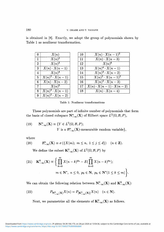
is obtained in [8]. Exactly, we adopt the group of polynomials shown by

Table 1 as nonlinear transformation.

0

1

2

3

4

5

6

7

8

9

X{n)

X{nfX{nf

X(n) • X(n

X{n)*X(n)2 • X(n

X(n) • X(n

X(nfX(n)3 X(nX{n)2 • X(n

- i )

- i )- 2 )

- i )- 2 )

10

11

12

13

14

15

16

17

18

X(n)

X{n)

X{n-

X(n

X(nfX{nfX{nfX{nf •

X(nfX(n) X(n

X(n).

•X(n

•X(nX(n

•X(n

- 1 ) .X{n

- i ) 2

- 3 )

- i )- 2 )

- i ) 2

- 3 )X(n - 2)- 4 )

Table 1: Nonlinear transformations

These polynomials are part of infinite number of polynomials that form

the basis of closed subspace N!^OO(X) of Hubert space L2(Ω, β, P) ,

(19)

where

(20)

Y is a β"oo(X)-measurable random variable},

= σ ({X(m); m < n, 1 < j < d}) (n G Z).

We define the subset K ^ X ) of L2((l, B,P) by

(21)k-0

m

fc=0

e N*, ri< 0, po € N, pfc G N*(l < k < m) 1.

We can obtain the following relation between N?.OO(X) and K^.OO(X):

(22). PNo_ao{x)X(n) = P[Ko_oo{x)]X(n) (n G N).

Next, we parametrize all the elements of K^_OO(X) as follows.



https://doi.org/10.1017/S002776300000684X



Step 1: We define the subspace Λ of sequences whose terms are non-negative integer by

(23) Λ Ξ { p = (po,Pi,P2, 0; Po > 1, P» > 0 (ί > 1),

and pi = 0 without finite number of exceptions}.

For each p G Λ, we introduce a one-dimensional strictly stationaryprocess φp = (φp(n);n G Z) by

oo

(24) φp(n) = l[X(n-kγ*

and define the subset G of stochastic processes as

(25) G = {φp; p € A}.

Step 2: For all q € N, we define Λ,(c Λ) and Gq(c G) by

ί ^ 1(26) Λ9 = < p € Λ; 2^(fc + l)Pfe = 9 f '

I fc=o J(27) Gg = {φp; p € Λ9}.

We can express Λ and G as the direct sum of Λ , q = 1, 2,. . . and G g ,q = 1, 2,..., respectively:

(28) Λ = £ Λ,,

(29) σ

Step 3: We introduce the lexicographical order into Λ. For any p, γl G Λ,

we arrange them by comparing q = Σ(k + l)pfc? q1 = Σ(& + l)pjfe

That is, if q > q1', we denote p > p'. If g = g7, we arrange them by

comparing {pfc} and {pj .} according to the lexicograpical order.

Step 4: In the same way, we arrange all the elements of G as follows

(30) G = {φf, j = 0,1,2,...}.



https://doi.org/10.1017/S002776300000684X



The polynomials shown in Table 1 are the first nineteen elements of

GQ that are arranged according to the above order. Note that φo = X.

Roughly speaking, these polynomials are arranged in the order of similarity

to the original strictly stationary process X = (X(n) n G Z).

We define a d+1-dimensional stochastic process X^oni = (^nonl(n)>n ^Z) by

φo(n)

( 3 1 ) v w ^ ^ _ Ψι{n) - E\Ψι{n)]

φd(n) - E[φd(n)] j

The following theorem shows that the closed subspace K^.OO(X) can be

approximated by the linear subspaces M ^ ^ X J ^ , ) (N 6 N*, d G N).

THEOREM 2.2. ([8]) The following relation holds:

(32) U U M%lN=0d=l

Given a one-dimensional time series X — (X(n)]0 < n < N), we

constitute various kinds of multi-dimensional time series, for example,

(33) - 1)); l<n<

We represent the above nonlinear transformation by the symbol of

(0, l,3)-type. Now, we can derive a KM2θ-Langevin equation from the

transformed time series, which we call nonlinear KM2 O-Langeυin equation.

§3. Causality analysis

In this section we give a short review of the causality analysis in the

theory of KM2θ-Langevin equations and its applications to real data [7].

We also give a more precise criterion for Test(CS) in view of statistical data

analysis.

3.1. The definition of causality

Let (Ω, 25, P) be a probability space. Suppose that we have two Re-

valued stochastic process X = (X(n); —00 < n < r) and R-valued stochas-

tic process Y = (Y(n); -00 < n < r) on (Ω, #, P). We define the causality

as follows.



https://doi.org/10.1017/S002776300000684X



DEFINITION 3.1. There exists causality that X is cause and Y is result

if for all n(—oo < n < r), there exists a Borel function Fn with infinite

number of variables such that

(34) Y(n) = Fn(X(n),X(n-l),...) a.s.

We denote the above relation as

(c)(35) X > Y.

If each component of X and Y is square integrable, then the definition

of causality is equivalent to

(36) N ^ ( Y ) C N^CX) (-00 < Vn < r).

3.2. Linear causality

We define the linear causality as a special case of causality definedabove, that is, Fn in (34) is linear. The linear causality that X is cause andY is result is equivalent to

(37) M ϋ ^ Y ) C M ^ X ) (-00 < Vn < r).

We denote the above relation as

(LC)

(38) X > Y.

The algorithm to check the linear causality is given in the theory ofKM2θ-Langevin equations. Let X = (X(n); — oo < n < r) and Y =(y(n); —oo < n < r) be Revalued and R-valued stochastic processes on(Ω, β, P), respectively. We assume that

(39) U = (C/(n); n e Z) = C(Y(n), *X(n)); n e Z)

is a d + 1 dimensional weakly stationary process with mean 0. We define

three correlation matrix functions i?χ, i?2, R3 by

(40) i?i(n) ΞΞ E(X(nYX(0)) G M(d, d; R),

(41) R2(n) = E(Y(nYX(0)) € M(l, d; R),

(42) R3(n) = E(Y(n)Y(0)) G M(l, 1; R)



https://doi.org/10.1017/S002776300000684X


184 V. OKABE AND T. YAMANE

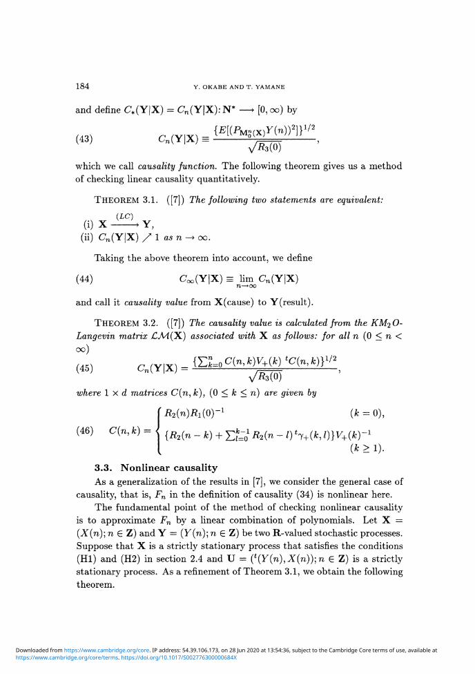
and define C*(Y|X) = Cn(Y|X):N* —> [0,oo) by

(43) Cn(Y|X) Ξ

which we call causality function. The following theorem gives us a methodof checking linear causality quantitatively.

THEOREM 3.1. ([7]) The following two statements are equivalent:

(LC)

( i )X >Y,(ii) Cn(Y|X) / 1 as n -> oo.

Taking the above theorem into account, we define

(44) CWY|X) = Urn C«(Y|X)n—•oo

and call it causality value from X(cause) to Y(result).

THEOREM 3.2. ([7]) The causality value is calculated from the KM^O-Langevin matrix £ΛΊ(X) associated with X as follows: for all n (0 < n <oo)

(45) Cn(Y|X) -

where 1 x d matrices C(n, k), (0 < k < n) are given by

)Ri(0)~1 {k = 0),

(46) C(n, fc) ={^(n-AJ + ΣίLo

(k > 1).

3.3 Nonlinear causalityAs a generalization of the results in [7], we consider the general case of

causality, that is, Fn in the definition of causality (34) is nonlinear here.The fundamental point of the method of checking nonlinear causality

is to approximate Fn by a linear combination of polynomials. Let X =(X(n)\ n G Z) and Y = (Y(n); n G Z) be two R-valued stochastic processes.Suppose that X is a strictly stationary process that satisfies the conditions(HI) and (H2) in section 2.4 and U = ^(Y^.X^y.n e Z) is a strictlystationary process. As a refinement of Theorem 3.1, we obtain the followingtheorem.



https://doi.org/10.1017/S002776300000684X



THEOREM 3.3. These two statements are equivalent:

(c)(i) X > Y,

(ii) C

(c)Proof. From the definition of nonlinear causality (34), X > Y is

equivalent to

that is,

(47) v

From the stationarity of U,

nonl '

w ^ ( 0 ) } 2 ]

This value increases monotonically with respect to TV and d. Thus, we

obtain

lim Cw(Y|xS2a)= limίlima,fy—ôo a—> oo iv—ôo

= lim Ca—ôo

Applying Theorem 2.2, we obtain

(48) E[{PM0 w F(0)}2] / E[{Pκo ( x ) y(0)} 2 ] as d, N - oo.

Since the mean vector of Y(0) is 0, we can get from (22)

(49) PNo_ xjYίO) = P[KOoΰ(x)]Y(0).

Therefore, by (47), (48), (49), we can complete the proof. Π

Thus, we can check the nonlinear causality approximately by reducing

it to the linear causality between Xônl(cause) and Y(result).



https://doi.org/10.1017/S002776300000684X



3.4. Data analysis: Test(CS)

Let X and Y be d-dimensional and one-dimensional stochastic process,

respectively, and X = {X(n)\ 0 < n < N} and y = {^(n); 0 < n < N}

be their corresponding time series. We assume that the (d+ l)-dimensional

data {t{y{n)^tX{n))]Q < n < N) passes Test(S) and can be regarded as

a realization of (d + l)-dimensional stationary process t(Y(n),tX(n)). We

discuss here an application of causality analysis to actual data analysis,

which we call Test(CS).

We can estimate the causal function Cn(Y|X) from data sets using

the algolithm of the fluctuation-dissipation theorem and Theorem 3.2. We

denote this estimator for the causal function by Cn(Y|X) or Cn(y\X).

These estimator are obtained by replacing the correlation matrix functions

in (46) with the sample correlation matrix function defined by (17) and

(18).

In data analysis, however, we find some difficulties that come from the

fact that the number of available data is finite. First, the number of reli-

able sample correlation matrix function in (17), (18) is limitted. From the

empirical knowledge in time series analysis, the domain of reliable sample

correlation matrix function of ( ί(y(n), ίA'(n));0 < n < N) is limitted to

{-M,..., 0,..., M}, where

(50) M = [3y/W+Ί/(d + 1)] - 1 (< N).

Secondly, we cannot calculate the limit in the definition of causality value

(44). Instead, we replace n —» oo with n = M, and adopt CM{y\X) as

an approximate value to the causality value COo(3 | )- We call CM{y\X)

sample causality value. Given two R-valued time series y and A', it should

be noted that we must check the stationarity of (^(^(n), Λnonlί72))' ^ — n —

N) as well as X when we calculate C^{y\X^nl), where M = [3y/N + l/d+

In actual data analysis, in order to check nonlinear causality, we calcu-

late all sample causality values between y and possible nonlinear transfor-

mations Xnon\i a n d find the maximum sample causality value.

Actually, because of finiteness of available data, we can only approx-

imate the underlying dynamics by nonlinear transformations. Therefore,

in actual data analysis, the sample causality value ^M^l^nonl) does not

reach 1 even if there exists a causal relation between given two time series.



https://doi.org/10.1017/S002776300000684X



Therefore, it is necessary to interpret the sample causality value according

to some criteria.

We must give up the idea of requiring a sample causality value to be

exact 1 even when there exists a causal relation. Instead, we check if sample

causality value is large enough for the two time series to have a causal

relation. In the following subsections, we describe some ideas of checking

this criteria.

3.5. Selection of effective variables

It gives us useful information to plot a sample causality function against

time. If the sample causality function is observed to saturate at some

time n in the plot, it is considered that the dynamics depends only on n

steps before, and the shortage of sample causality value toward 1, that is,

1 — Cn(y\X), is due to the fluctuation.

We can find an integer n = M' at which the sample causality func-

tion Cn{y\X) exceeds the 95% of CM{y\X) for the first time. We adopt

CM'(y\X) as a new sample causality value insted of that of n = M, and

rewrite M' as M.

3.6. Estimation of the confidence interval of a sample causal-

ity value

In this subsection, we give a method of estimating the confidence inter-

val of sample causality value based on the Bootstrap method [10], which has

been frequently used as a nonparametric method in statistical data analysis.

(i) It follows from the definition of the causality function (43) and the

strictly stationarity of U = (ί(Y'(n),tX(n)); n G Z) that the causal-

ity value CM(Y|X) depends on only the joint probability of (Y(n),

X(n),. . . , X(n — M)). The estimation of this joint probability distri-

bution is given by the following empirical distribution

(51) P(A) = ΛT \ £ ι Λ

n=M

Ae

where δz is the delta measure whose support is centered at z.

(ii) Next, we choose (d(M+l)+l)-dimensional (N — M+l) samplings with

displacement from the empirical distribution p. The concrete proce-

dure of choosing samples is that we select randomly an integer n from



https://doi.org/10.1017/S002776300000684X



{M,. ..,JV} and adopt the corresponding data set (^(n), X(n),...,X(n — Λf)) as a new sample.

(iii) Since these samples are considered to be L~ p, we can compute thequantities which might be called bootstrapped sample causality value.We repeat this procedure B times, and obtain the sequence of samplecausality values CΊ, . . . , Cβ

(iv) We can make a statistical inference of sample causality value CΆf (Y|X)by making the emprical distiribution of CΊ, . . . , Cβ- For example, wecan obtain a confidence interval of Cjvf (Y|X) by approximating thedistribution of CM(Y|X) ~~ C M ( Y | X ) by the empirical distiributionoiCi-CMQ>\X),i = l,...,B.

3.7. Criterion for the causal relations between two time series

In this subsection, we give a method of testing the null hypothesis thatthere are no causal relations between two time series.

The fundamental idea is that we compare the confidence interval of sam-ple causality value with the distribution of sample causality values underthe condition that there are no causal relations, and if these two distribu-tions are quite different from each other, we can reject the null hypothesis.If the causal time series X is replaced by a physical random sequence 7£,there would be no causal relations between y and TZ. In this case, we canmake the distribution of sample causality values by replacing the physicalrandom sequence TZ one after another.

Let Fι-2a be the upper 100(1 — 2α)% point of the distribution of samplecausality values between y and TZ and L\-2a be the lower bound of theconfidence interval of sample causality value in question. Comparing thesetwo quantities, we can reject the null hypothesis if

(52) Li_ 2 α > Fi_ 2 α .

§4. Finding underlying dynamics in time series

In this section, we describe a procedure to investigate the deterministicdynamics of time series.

4.1. Finding deterministic dynamics in time series: Test(D)

Suppose that we have a one-dimensional time series X = (A'(n) O <n < N) which is judged to be stationary by Test(S). The data X can beregraded as a realization of the underlying stationary stochastic process



https://doi.org/10.1017/S002776300000684X



X = (X(n) O < n < N). We define another stationary stochastic processX+ i = (X+i(n);0 < n < N - 1) by

(53) I + i ( n ) = X(n + 1), (0 < n < N - 1)

that is, we obtain X+χ by shifting time domain by one step into future. Xis called deterministic if there exists causality that X is cause and X + i isresult:

(c)(54) X >X+ 1.

We call the above method of checking determinism in time series Test(D).We should notice that the determinism of time series defined here does

not necessarily imply that it comes from a deterministic dynamic system,such as chaos. According to the definition of causality value (44), it meansthat the fluctuation flow occupies only small part of (nonlinear) KM2O-Langevin equation derived from X or ^onl* Therefore, even a time se-ries that comes from AR model can be judged to be deterministic by ourmethod.

4.2. Finding chaotic dynamics in time series

Let X = (X(n);0 < n < N) be a one-dimensional time series whichis judged to be deterministic by Test(D). Our concern here is to considerwhether the dynamics behind this time series is chaotic.

On the basis of deterministic time series prediction, it is argued in [1]that we can distinguish chaos from uncorrelated measurement error by timeseries prediction. Specifically, if prediction precision falls off as predictionstep becomes large, though near future of time series can be predicted withsufficiently high precision, the dynamics is thought to be chaotic. Whereas,if the prediction precision is independent of prediction step, the randomnessis due to measurement error.

In the same way, we can investigate the underlying chaotic dynamicsfrom the viewpoint of prediction analysis based on the theory of KM2O-Langevin equations as follows. First, we find the nonlinear KM^O-Langevinequation that approximates the time evolution of X the most precisely.Secondly, we divide the time series into two parts, one is for reference forprediction, and another is for comparison of predicted data with real data.We fix the prediction step, and repeat the prediction of X using the nonlin-ear KM2θ-Langevin equation. In order to evaluate the quality of forecasts,



https://doi.org/10.1017/S002776300000684X



two error estimators are introduced. One is the normalized mean square

root error C(T) defined by

C(T) = (iXpred(T) ~ (Xpved(T)))(xorg - (xoτg)))

where, T is a prediction step, xorg and xpreά(T) denote the the original data

and the predicted data with prediction step T, respectively. The other is

the normalized centered correlation coefficient E(T) between predicted and

real data defined by

(56) E{T) \\Xoτg — \Xoτgi

It follows that C(T) = 1 or E(T) = 0 means that the prediction is perfect,

while C(T) — 0 or E(T) = 1 means that prediction is quite useless. Finally,

we plot the above two quantities against prediction step T, and find the

relation between prediction precision and prediction step.

§5. The result of numerical experiments

In this section, we apply our method to time series from the natural

world. We treat the measles data and chickenpox data. The original data

are not judged to be stationary by Test(S). Therefore, in order to extract

stationarity, we transform them before data analysis as follows:

Difference: V(n) = U{n) - U{n - 1), (1 < n < N).

Standardization: W(n) = /R\ (V(n) - μv).

Arctangent: X(n) — arctan W(n), (0 < n < N).

Nonlinear transformation: y(n) — < nonl(n)> (0 n ^

Standardization: Z{n) — I * . I (y(n) — μy),

(0 < n < N).

We do not refer to Test(S), but all the time series which we deal with

here can be checked to be stationary by Test(S)([4]).



https://doi.org/10.1017/S002776300000684X



As is clear from (50) that gives the number of reliable sample corre-lation matrix function, a nonlinear transformation with large dimension dovershortens the domain of sample correlation matrix function Rκ. There-fore, we use only nonlinear KJV^O-Langevin equations whose dimensionsare smaller than three.

We repeat the bootstrap procedure B = 1000 times for both measlesdata and chickenpox data.

5.1. MeaslesHere, we deal with the time series of monthly cases of measles in New

York City from 1928 to 1963. The original data are shown in Figure 1.

30000

25000

20000 -

15000

10000

5000

50 100 150 200 250time (months)

300 350 400 450

Figure 1: Data of measles

The data have a conspicuous peak around n = 160. This suggests thatthe inner structure of time series changes around n = 160. In fact, thewhole time series that contains data around n = 160 cannot be judged tobe stationary for the above transformations. Therefore, we split the timeseries around n = 160 into two parts; one is from n = 0 to n = 150 (I) andthe other is after n = 160 (II), and analyse them separately. Both (I) and(II) are judged to be stationary by Test(S) under the above transformations.

First, we perform Test(D) for (I) and for (II). The maximum sample



https://doi.org/10.1017/S002776300000684X



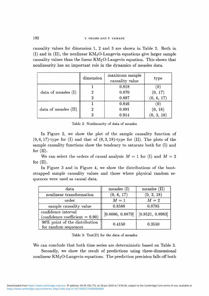
causality values for dimension 1, 2 and 3 are shown in Table 2. Both in

(I) and in (II), the nonlinear KM2θ-Langevin equations give larger sample

causality values than the linear KM^O-Langevin equation. This shows that

nonlinearity has an important role in the dynamics of measles data.

data of measles (I)

data of measles (II)

dimension

1

2

3

1

2

3

maximum sample

causality value

0.818

0.870

0.887

0.846

0.891

0.914

type

(0)(0, 17)

(0, 6, 17)

(0)(0, 18)

(0, 3, 18)

Table 2: Nonlinearity of data of measles

In Figure 2, we show the plot of the sample causality function of

(0,6,17)-type for (I) and that of (0,3,18)-type for (II). The plots of the

sample causality functions show the tendency to saturate both for (I) and

for (II).

We can select the orders of causal analysis M = 1 for (I) and M = 2

for (II).

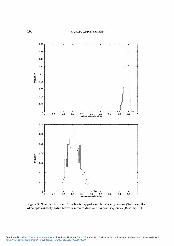
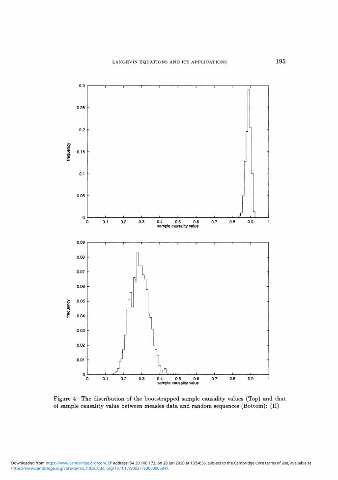
In Figure 3 and in Figure 4, we show the distributions of the boot-

strapped sample causality values and those where physical random se-

quences were used as causal data.

data

nonlinear transformation

order

sample causality value

confidence interval(confidence coefficient = 0.90)90% point of the distributionfor random sequences

measles (I)

(0, 6, 17)

M = 1

0.8588

[0.8086, 0.8879]

0.4150

measles (II)

(0, 3, 18)

M = 2

0.8785

[0.8521, 0.8983]

0.3550

Table 3: Test(D) for the data of measles

We can conclude that both time series are deterministic based on Table 3.

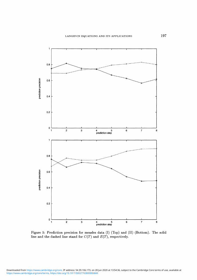
Secondly, we show the result of predictions using three-dimensional

nonlinear KM2θ-Langevin equations. The prediction precision falls off both



https://doi.org/10.1017/S002776300000684X



Figure 2: Sample causality functions for measles data (I) (Top) and (II) (Bottom)



https://doi.org/10.1017/S002776300000684X



0.18

0.1 0.2 0.3 0.4 0.5 0.6 0.7 0.8 0.9 1

0.07

0.06 -

0.05 -

0.04

- 0.03

0.02

0.01 -

0.2 0.3 0.4 0.5 0.6sample causality value

0.7 0.8 0.9

Figure 3: The distribution of the bootstrapped sample causality values (Top) and thatof sample causality value between measles data and random sequences (Bottom): (I)



https://doi.org/10.1017/S002776300000684X



0.25

0.15 -

0.05 -

0.1 0.2 0.3 0.4 0.5 0.6sample causality value

0.7 0.8 0.9

0.09

0.08

0.07

0.06

0.05 -

I 0J0.04 -

0.03 -

0.02 -

0.01

0.1 0.2

I

0.3 0.4 0.5 0.6sample causality value

0.7 0.8 0.9

Figure 4: The distribution of the bootstrapped sample causality values (Top) and thatof sample causality value between measles data and random sequences (Bottom): (II)



https://doi.org/10.1017/S002776300000684X



in (I) and in (II) as the prediction step increases. Therefore, the dynamicsboth in (I) and in (II) are thought to be chaotic.

In conclusion, we can assert that the data of measles is not only de-terministic but also chaotic. Comparing the result of experiments for (I)and for (II), we can infer that the fluctuation flow of (I) occupies the largerpart of the dynamics than that of (II), though the fundamental structureof dynamics seems to be unchanged throughout (I) and (II).

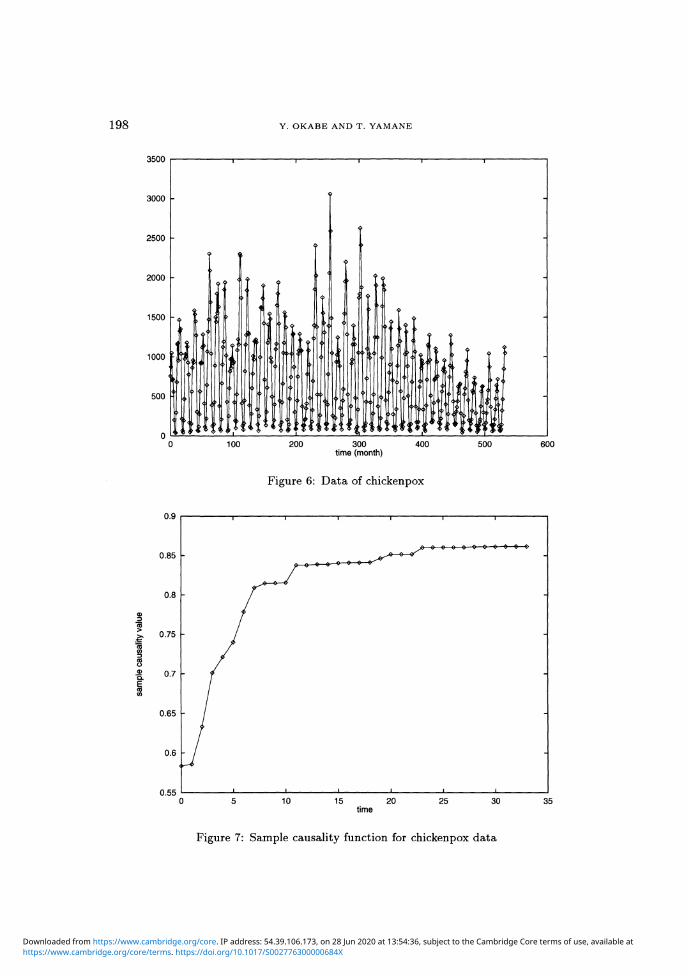
5.2. Chickenpox

Here, we deal with the time series of monthly cases of chickenpox inNew York City from 1949 to 1972. The original data are shown in Figure 6.

We repeat the same procedure which was performed for the measlesdata.

First, we perform Test(D). The maximum sample causality values fordimension 1, 2 and 3 are shown in Table 4. In contranst with measlesdata, the nonlinear KM2θ-Langevin equations give almost the same samplecausality values as the linear KM2θ-Langevin equation. This shows thatnonlinearity has no important meaning in the dynamics of chickenpox data.

data of chickenpox

dimension

123

maximum samplecausality value

0.8610.8730.881

type

(0)(0, 13)

(0, 8, 18)

Table 4: Nonlinearity of data of chickenpox

We show in Figure 7 the plot of the sample causality function for thelinear KM^O-Langevin equation. The plot of the sample causality functionshows the tendency to saturate.

We can select the orders of causal analysis M = 8 for the data ofchickenpox.

In Figure 8, we show the distribution of the bootstrapped samplecausality values and that where physical random sequences were used ascausal data.



https://doi.org/10.1017/S002776300000684X



4 5prediction step

4 5prediction step

Figure 5: Prediction precision for measles data (I) (Top) and (II) (Bottom). The solidline and the dashed line stand for C(T) and E(T), respectively.



https://doi.org/10.1017/S002776300000684X



3500

3000 -

2500

2000

1500

1000

500

Figure 6: Data of chickenpox

0.85

0.75 -

0.65

0.6 -

0.5515 20

time

Figure 7: Sample causality function for chickenpox data



https://doi.org/10.1017/S002776300000684X



0.25 -

0.15 -

0.05 -

0.1 0.2 0.3 0.4 0.5 0.6sample causality value

0.7 0.8 0.9

0.08

0.07 -

0.06

0.05

0.04 •

0.03

0.02 -

0.01

0.1 0.2 0.3 0.4 0.5 0.6 0.7 0.8 0.9

Figure 8: The distribution of the bootstrapped sample causality values (Top) and thatof sample causality value between chickenpox data and random sequences (Bottom)



https://doi.org/10.1017/S002776300000684X



data

nonlinear transformationorder

sample causality valueconfidence interval(confidence coefficient = 0.90)

90% point of the distribution for random sequences

chickenpox

(0)

M = 80.8146

[0.7789, 0.8227]

0.3350

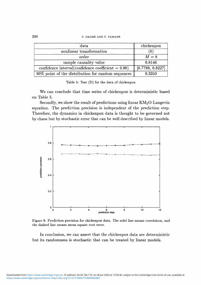
Table 5: Test (D) for the data of chickenpox

We can conclude that time series of chickenpox is deterministic basedon Table 5.

Secondly, we show the result of predictions using linear KM2θ-Langevinequation. The prediction precision is independent of the prediction step.Therefore, the dynamics in chickenpox data is thought to be governed notby chaos but by stochastic error that can be well described by linear models.

prediction step

Figure 9: Prediction precision for chickenpox data. The solid line means correlation, andthe dashed line means mean square root error.

In conclusion, we can assert that the chickenpox data are deterministicbut its randomness is stochastic that can be treated by linear models.



https://doi.org/10.1017/S002776300000684X


LANGEVIN EQUATIONS AND ITS APPLICATIONS 2 0 1

REFERENCES

[1] G. Sugihara and R. M. May, Nonlinear forecasting as a way of distinguishing chaosfrom measurement error in time series, Nature, 344 (1990), 734-741.

[2] P. Masani and N. Wiener, Non-linear prediction, Probability and Statistics,, TheHarald Cramer, (V. Grenander, ed.), John Wiley, 1959, pp. 190-212.

[3] Y. Okabe, On a stochastic difference equation for the multi-dimensional weaklystationary process with discrete time, Prospect of Algebraic Analysis, (M. Kashiwaraand T. Kawai, eds.), Academic Press, Tokyo, 1988, pp. 601-645.

[4] Y. Okabe and Y. Nakano, The theory of KM2 O-Langeυin equations and its applica-tions to data analysis (I): Stationary analysis, Hokkaido Math. J, 20 (1991), 45-90.

[5] Y. Okabe, Application of the theory of KM2 O-Langeυin equations to the linear pre-diction problem for the multi-dimensional weakly stationary process, J. Math. Soc.of Japan, 45 (1993), 277-294.

[6] Y. Okabe, Langevin equations and causal analysis, SUGAKU Exposition, Amer.Math. Soc. Transl., 161 (1994), 19-50.

[7] Y. Okabe and A. Inoue, The theory of KM2 O-Langeυin equations and its applicationsto data analysis (II): causal analysis (1), Nagoya Math J., 134 (1994), 1-28.

[8] Y. Okabe and T. Ootsuka, Applications of the theory of KM2 O-Langeυin equationsto the nonlinear prediction problem for the one dimensional strictly stationary timeseries, J. Math. Soc. Japan, 47 (1995), 349-367.

[9] Y. Okabe, Non-linear time series analysis based upon the fluctuation-dissipation the-orem, Nonlinear Analysis, Theory, Method & Applications, 30 (1997), 2249-.

[10] B. Efron, Bootstrap methods: Another look at the jackknife, The Annals of Statistics,7 (1979), 1-28.

Yasunori OkabeDepartment of Mathematical Engineering and Information PhysicsGraduate School and Faculty of EngineeringUniυersity of TokyoBunkyo-ku, Tokyo 113Japan

Toshiyuki YamaneDepartment of Mathematical Engineering and Information PhysicsGraduate School and Faculty of EngineeringUniυersity of TokyoBunkyo-ku, Tokyo 113Japan



https://doi.org/10.1017/S002776300000684X


y. okabe and t. yamane - cambridge university press...y. okabe and t. yamane nagoya math. j. vol....

Documents