y. hatta, e. iancu, k. itakura and l. mclerran- odderon in the color glass condensate

8/3/2019 Y. Hatta, E. Iancu, K. Itakura and L. McLerran- Odderon in the Color Glass Condensate

http://slidepdf.com/reader/full/y-hatta-e-iancu-k-itakura-and-l-mclerran-odderon-in-the-color-glass 1/43

a r X i v : h e p - p h / 0 5 0 1 1 7 1 v 1 1

8 J a n 2 0 0 5

SPhT-T05/010

BNL-NT05/1

Odderon in the Color Glass Condensate

Y. Hatta

RIKEN BNL Research Center, Brookhaven National Laboratory, Upton, NY

11973, USA

E. Iancu 1 , K. Itakura

Service de Physique Theorique, CEA Saclay, 91191 Gif-sur-Yvette, France

L. McLerranPhysics Department and RIKEN BNL Research Center, Brookhaven National

Laboratory, Upton, NY 11973, USA

Abstract

We discuss the definition and the energy evolution of scattering amplitudes with C -

odd (“odderon”) quantum numbers within the effective theory for the Color GlassCondensate (CGC) endowed with the functional, JIMWLK, evolution equation.We explicitly construct gauge-invariant amplitudes describing multiple odderon ex-changes in the scattering between the CGC and two types of projectiles: a color–singlet quark–antiquark pair (or ‘color dipole’) and a system of three quarks in acolorless state. We deduce the energy evolution of these amplitudes from the gen-eral JIMWLK equation, which for this purpose is recast in a more synthetic form,which is manifestly infrared finite. For the dipole odderon, we confirm and extendthe non–linear evolution equations recently proposed by Kovchegov, Szymanowskiand Wallon, which couple the evolution of the odderon to that of the pomeron, andpredict the rapid suppression of the odderon exchanges in the saturation regime at

high energy. For the 3–quark system, we focus on the linear regime at relatively lowenergy, where our general equations are shown to reduce to the Bartels–Kwiecinski–Praszalowicz equation. Our gauge–invariant amplitudes, and the associated evo-lution equations, stay explicitly outside the Mobius representation, which is theHilbert space where the BFKL Hamiltonian exhibits holomorphic separability.

1 Membre du Centre National de la Recherche Scientifique (CNRS), France.

Preprint submitted to Elsevier Science 2 February 2008

http://arxiv.org/abs/hep-ph/0501171v1


































1 Introduction

Since the advent of the Balitsky–Fadin–Kuraev–Lipatov (BFKL) equation[1,2] in the mid seventies, there has been significant progress in our compre-

hension of high–energy QCD, and several theoretical approaches have beenproposed which aim at a resummation of the energy–enhanced radiative cor-rections to high–energy processes in perturbative QCD. The BFKL equationis a leading logarithmic approximation (LLA), which allows one to resum to allorders corrections of the form (αs ln s)n to the scattering between two colorlessobjects via the exchange of two gluons in the t–channel. As a result of thisresummation, the bare two–gluon exchange is replaced by the BFKL pomeron

(the sum of an infinite series of ladder diagrams of ordinary perturbation the-ory), or, equivalently, by two reggeized gluons which interact with each other.All the subsequent theoretical approaches proposed within perturbative QCDencompass the BFKL equation, and can be viewed as extensions of the latter

towards increasing the complexity of the objects exchanged in the t–channel,and also towards enlarging the limits of the LLA.

The simplest object beyond the BFKL pomeron within perturbative QCD isthe exchange of three interacting (reggeized) gluons in a symmetric color state.This object, which is negative (or “C –odd”) under charge conjugation (C =−1), represents the lowest order perturbative contribution to the odderon , theC –odd exchange which dominates the difference between the hadronic crosssections for direct and crossed channel processes at very high energies [3].The evolution of the three–gluon odderon exchange with increasing energy in

the LLA is described by the BKP equation, established by Bartels [4] andKwiecinski and Praszalowicz [5], which amounts to a pairwise iteration of the BFKL kernel (see also [6]). This equation can be immediately extendedto describe the exchange of an arbitrary number n ≥ 3 of reggeized gluonswith pairwise BFKL interactions [7,4,8,9,10]. The resulting formalism, alsoknown as the generalized leading logarithmic approximation (GLLA), resumsall radiative corrections that involve the maximally possible number of energylogarithms ln s for a given number of exchanged gluons. At the moment, twoexact solutions of the BKP equation for odderon evolution are available [11,12],and the subject continues to be under intensive debate [13,14] (see also therecent review paper [15] and the discussion below).

In the formalisms described so far, the number of gluons in the t-channelremains fixed in the course of the evolution. This is probably a good ap-proximation in some intermediate kinematical region, but it fails to describetwo interesting physical situations: First, it does not incorporate correctly the fluctuations in the number of gluons, as resulting from processes in which one(reggeized) gluon splits into two, or, more generally, a n–gluon state evolvesinto a (n + m)–one, with m ≥ 1. Such processes are especially important

2



in the dilute regime at relatively large transverse momenta (for a given en-ergy), where gluon splitting is the main process through which higher–pointcorrelations get built [16]. Second, the approximation in which the numberof t–channel gluons is fixed cannot describe recombination processes in which(reggeized) gluons merge with each other, thus reducing the gluon density.

Such processes are important in the high–energy regime where the gluon den-sity becomes large enough (due to BFKL evolution and to the splitting pro-cesses alluded to above) to enhance recombination processes, which are thenexpected to lead to gluon saturation [17,18,19]. The inclusion of saturation isalso necessary, for consistency, in studies of the unitarization of the scatteringamplitudes, except for some exceptional kinematical configurations [20].

The simplest approach including gluon splitting in the framework of BFKLevolution is the color dipole picture developed by Mueller [20,21]. This pictureis valid at large N c, and describes pomeron multiplication via vertices at which

one (BFKL) pomeron splits into two. A more ambitious program, which is notrestricted to the large–N c approximation, is the extended generalized leading

logarithmic approximation (EGLLA), initiated by Bartels [22], in which thegluon number changing vertices are explicitly computed in perturbative QCD(see Refs. [23,24,25,26,27,28,29] for further developments along this line andRef. [15] for a review). By using such vertices, evolution equations allowing forgluon splitting have been written down in Refs. [24,27,29]. Also, the equiva-lence between the triple pomeron vertex in the dipole picture [21,30] and theone generated by EGLLA at large N c [23,25] has been verified in Refs. [24,28].

So far, the only formalism allowing for the systematic inclusion of gluon merg-ing in the high–energy evolution is the Color Glass Condensate (CGC) [31], inwhich the reggeized gluons are replaced by classical color fields whose correla-tions get built in the course of the evolution. But the corresponding evolutionis non–linear : the new gluons radiated at one step in the evolution (the analogof the ‘rungs’ in the BFKL ladders) are allowed to scatter off the classical colorfields generated in the previous steps, and this is the mechanism leading togluon merging. Because of the non–linear effects, the evolution couples n–pointfunctions with various values of n, and can be most compactly summarizedas a functional Fokker–Planck equation for the weight function describing thecorrelations: the Jalilian-Marian–Iancu–McLerran–Weigert–Leonidov–Kovner

(JIMWLK) equation [32,33,34]. Alternatively, and equivalently [35], the evolu-tion can be formulated as an hierarchy of equations for scattering amplitudes— the Balitsky equations [36] —, in which unitarity is manifest. Note how-ever that gluon splittings are not included in the JIMWLK equation [16]; thisis obvious from the fact that, in the dilute, or weak–field , limit, this equa-tion reduces to an evolution in which the number of gluons in the t–channelstays constant [33,37]. An extension of the JIMWLK–Balitsky evolution whichincludes pomeron splitting has been proposed only very recently [16,38].

3



As it should be clear from this succinct presentation, the various formalismsproposed so far in perturbative QCD at high energies are quite different fromeach other, and the correspondences between them are not always transpar-ent. We know for instance that all these approaches reproduce the Balitsky–Kovchegov (BK) equation [36,39], which is the simplest non–linear generaliza-

tion of the BFKL equation, but only in the sense of a mean field approximationthat has been recently challenged [16,40,41,42]. But the relation between thecorrelations (i.e., the n–point functions with n > 2) generated by the differ-ent approaches is much less understood. For instance, it has been shown onlyrecently, by Kovchegov, Szymanowski and Wallon [43], that the perturbativeodderon can be accommodated within Mueller’s dipole picture [20], and thatthe corresponding solution coincides with the Bartels–Lipatov–Vacca (BLV)solution [12] to the BKP equation.

In particular, in the regime where saturation effects can be neglected, oneexpects the CGC formalism and the more traditional approaches like GLLA

to be equivalent with each other, but this has never been verified beyond theexample of the 2–point function (i.e., of the BFKL equation). With this paper,we would like to make one more step towards elucidating this correspondence,by establishing the equivalence between the two approaches at the level of odd-

eron exchanges (i.e., for a 3–point function). Specifically, we shall demonstratethat, in the weak–field limit , the JIMWLK evolution of the C –odd three–gluonexchanges reduces to the BKP equation, as expected.

But recovering the BKP equation from the CGC formalism is not the mainpurpose of the present analysis, but only a pretext for it. The CGC is the

theoretical framework par excellence for a study of high–energy scatteringand evolution in QCD near the unitarity limit, yet the odderon problem hasnever been addressed in this formalism before. Thus, a substantial fractionof the subsequent analysis will be devoted to the proper formulation of theodderon exchanges in the framework of the CGC, and to the derivation of thecorresponding evolution equations from the general, JIMWLK, equation. Thisstudy of the odderon should be a good starting point towards understandingthe multi–reggeon dynamics within the CGC formalism.

Our study will also emphasize some essential differences between the CGC for-malism and the perturbative approach based on the BFKL Hamiltonian: The

latter is adapted to the description of a single scattering via the exchange of acomposite object — pomeron, odderon, or, in general, a system of n reggeizedgluons — which evolves with increasing energy. It relies on “kT –factorization”(see, e.g., [44]) to separate the dynamics in the transverse plane from that inthe longitudinal direction, and express a scattering amplitude as the convolu-tion of an universal Green’s function , which describes the exchanged object,with the process–dependent impact factors, which connect this object to theexternal particles. From the above, one sees that the calculation is most nat-

4



urally carried on in momentum space.

By contrast, in the CGC formalism — which is specially tailored to describeunitarity corrections —, single and multiple scatterings are treated on thesame footing, namely they are resummed in process–dependent, and gauge–

invariant, scattering amplitudes, which are computed in the eikonal approxi-mation , and thus are naturally constructed in coordinate space. There is nokT –factorization any longer, nor universal Green’s functions: the longitudinaland transverse dynamics are tied up together in Wilson lines, which describethe eikonal scattering of the elementary particles which compose the projectile

(the external object which scatters off the CGC, identified as the target ).

These differences explain some of the subtleties that we shall meet when tryingto compare results for the odderon in the two approaches. On one hand, theodderon is described by the universal Green’s function of three reggeized glu-ons, which obeys BKP equation in momentum space. On the other hand, the

CGC scattering amplitudes depend upon the specific process at hand (theyinclude the impact factor of the projectile) and obey non–linear evolutionequations written in coordinate space. (In general, these are not closed equa-tions, but just a part of Balitsky’s hierarchy [36].) Still, in the weak–field, orsingle–scattering, approximation, in which the evolution equations become lin-ear, they must contain the same non–trivial information as the BKP equation,whatever is the process under consideration.

The authors of Ref. [43] have met with a similar difficulty when trying tocompare the C –odd scattering amplitude of a dipole with the standard BKP

odderon. In that case, they have been able to do so by using the respectivesolutions, which are explicitly known. Here, we shall follow a more generalstrategy, which applies to arbitrary processes, including those where the evo-lution equations are too complicated to be solved exactly. Namely, by inspec-tion of two specific processes, we shall be able to identify the analog of theuniversal odderon Green’s function in the weak–field limit of the CGC for-malism, and show that, when properly defined, this quantity obeys indeed the(coordinate version of the) BKP equation. As we shall momentarily explain,this CGC approach to the BKP equation not only establishes a correspon-dence between the two formalisms, but also reveals some new insights aboutthe BKP equation itself.

The two specific processes that we shall consider are the CGC scattering witha quark–antiquark color dipole (a sub–process of the virtual photon—CGCscattering) and that with a colorless 3–quark system (a simple model for abaryon). For both cases we start by constructing the general, non–linear, am-plitudes which describe multiple odderon exchanges (these turn out to be theimaginary parts of the respective S –matrix elements, themselves expressedin terms of Wilson lines), and then expand these amplitudes in the limit

5



where the CGC field is weak. After this expansion, both amplitudes reduce to(gauge–invariant) linear combinations involving a three–gluon Green’s func-tion in a totally symmetric color state. Clearly, this Green’s function is anatural candidate for the BKP odderon in the CGC formalism. This inter-pretation is, however, hindered by the fact that the CGC Green’s functions

are gauge–variant objects, for which the JIMWLK equation predicts infraredsingularities (to be contrasted with the BKP equation, which is infrared safe).Although physically harmless — as they cancel in the gauge–invariant am-plitudes —, these singularities complicate the correspondence with the BKPapproach.

At this point comes one of the main new technical developments in this paper:We show that the JIMWLK Hamiltonian [33,34] can be rewritten in a newform, which is manifestly infrared finite (the original kernel in the transversespace is replaced by the dipole kernel [20], which decays much faster at largedistances). When acting on gauge–invariant quantities, this new Hamiltonian

is equivalent with (but simpler to use than) the original one, in the sense of generating the same evolution equations. But the new Hamiltonian generatesinfrared–finite equations also for the gauge–variant Green’s functions, and thusallows us to introduce the latter in a mathematically well–defined way. Withthis prescription, the equation satisfied by the CGC odderon Green’s functionturns out to be the same as the Fourier transform to coordinate space of theBKP equation, as we shall check explicitly.

But this Fourier transform reserves some more surprises, as it could be an-ticipated from the fact that our equation in coordinate space is not exactly

the same as the coordinate–space version of the BKP equation that is usuallywritten in the literature 2 (see, e.g., [15]). Rather, the two equations coincidewith each other only if we require our CGC Green’s function, which in gen-eral is a totally symmetric function of three transverse coordinates, to vanishwhenever two coordinates become identical. This property is sometimes re-ferred to as “the Mobius representation” (see, e.g., [28]), and is interestingin that, when restricted to functions having this property, the BFKL Hamil-tonian is conformally invariant [2] and exhibits holomorphic separability [8].This mathematical simplification has led [9,10] to a powerful analogy betweenthe BKP odderon problem (and, more generally, the problem of multi–reggeonexchanges in the limit of a large number of colors) and an integrable Heisen-

berg spin chain. In particular, the first exact solution to the BKP equationhas been found, by Janik and Wosiek [11], by exploiting this analogy.

2 At the technical level, the difference originates in some ambiguities in the formof delta–functions which appear when Fourier transforming the momentum–spaceBKP equation to coordinate space, and which are generally interpreted in the senseof the Mobius representation [28]; that is, these delta–functions are simply ignored.

6



But although natural for the pomeron exchange (i.e., at the level of the 2–pointfunction), where it entails no loss of generality, the restriction to the Mobiusrepresentation is not so natural for the higher n–point functions (n ≥ 3), asrecently emphasized in Ref. [28]. For instance, the other known solution tothe BKP equation, due to Bartels, Lipatov, and Vacca [12], which dominates

at high energy and is perhaps of more relevance for the phenomenology (as itcouples to a virtual photon), lies outside the Mobius representation.

Similarly, the use of the Mobius representation does not appear to be naturalin the CGC formalism either. In fact, our both examples of gauge–invariantscattering amplitudes lie outside this representation: For the dipole case, thereis no coupling to this functional space, as well known [12,43], whereas for the3–quark case, this property is excluded by the initial conditions. We concludethat, at least for the problems that we shall discuss, the BKP equation mustbe solved in a Hilbert space more general than the Mobius representation.

But our analysis below will not be confined to the weak–field limit and its re-lation with the perturbative QCD approaches. As repeatedly emphasized, theCGC is a formalism for multiple scattering, in which non–linear amplitudesand the corresponding evolution equations are straightforward to construct.As an illustration, we shall derive the general evolution equations for thescattering amplitudes describing C –odd and, respectively, C –even exchangesin the dipole–CGC scattering (the non–linear generalizations of the odderonand, respectively, pomeron exchanges). In fact, these equations will be ob-tained by simply separating the real part and the imaginary part of the firstequation in the Balitsky hierarchy [36]. Interestingly, the non–linear terms in

these equations are found to couple the odderon and pomeron evolutions. Inthe mean field approximation in which the non–linear terms are assumed tofactorize, the equation for the C –odd amplitude reduces to a non–linear equa-tion originally proposed in Ref. [43]. Our analysis of this equation will confirmthe conclusion [43] that the odderon exchanges are strongly suppressed by theunitarity corrections, and will allow us to deduce the mathematical law forthis suppression. For the 3–quark system, we shall not write down the corre-sponding non–linear equation (since this appears to be too complicated to beilluminating). Rather, we shall rely on the relation between the correspondingC –odd amplitude and the respective one for the dipole to conclude that, in theweak–field regime, the dominant increase with the energy should be controlled

again by the BLV solution [12], so like for the dipole case [43].

The plan of the paper is as follows. In Sect. 2 we give a general proof that theJIMWLK evolution of gauge–invariant observables is free of infrared problems,and we deduce an alternative form of the JIMWLK Hamiltonian which makesinfrared finiteness manifest. In Sect. 3, we consider the weak–field limit of theJIMWLK evolution, and show that the use of the new Hamiltonian allowsone to introduce well–defined CGC Green’s functions. In Sect. 4 we construct

7



the general amplitudes describing multiple C –odd exchanges for a color dipoleand a 3–quark system. Then, in Sects. 5 and 6, we deduce the correspondingevolution equations, after having introduced first the odderon Green’s functionin the CGC. Finally, in Sect. 7 we discuss the connection to the BKP equation.

2 The JIMWLK equation with the dipole kernel

In this section, we show that the JIMWLK equation can be considerably sim-plified when its action is restricted to gauge–invariant correlation functions,such as the scattering amplitudes. The resulting equation is still a functionaldifferential equation, but with a different kernel in transverse space — thedipole kernel —, which has a more rapid fall–off at large distances, and there-fore makes it easier to check that the evolution is free of infrared singularities.

2.1 The JIMWLK equation

The CGC formalism [31] is an effective theory for the small–x gluons in thelight–cone wavefunction of an energetic hadron. In this formalism, the gluonswith small longitudinal momenta, or small values of x, are described as theclassical color field radiated by ‘color sources’ (gluons and valence quarks) withhigher values of x, which are ‘frozen’ by Lorentz time dilation in some randomconfiguration. Accordingly, the color fields at small–x are themselves random,with a distribution specified by the ‘weight function’ W τ [α] (a functional prob-ability density). Here, τ ≡ ln(1/x) is the rapidity, and α ≡ αa(x−,x) is thelight–cone component of the color gauge field, and is the only non–trivial com-ponent in a suitable gauge (the ‘covariant gauge’; see below). Note that thisfield depends upon the light–cone longitudinal coordinate 3 x− ≡ (t − z)/

√2,

and upon the transverse coordinates x = (x, y), but not upon the (light-cone)time x+ ≡ (t + z)/

√2, in agreement with the ‘freezing’ property mentioned

above.

All the interesting physical quantities are expressed as operators built with α,say O[α], and the corresponding expectation values are obtained after aver-

aging over the random field α:

Oτ ≡

Dα O[α] W τ [α]. (2.1)

Whereas, by itself, the weight function W τ [α] is a non–perturbative object, itsevolution with decreasing x (or increasing energy) can be computed in pertur-

3 We assume that the color glass moves in the positive z direction.

8



bation theory, at least in the high energy regime where the intrinsic ‘saturationmomentum’ Qs(x) (which increases as a power of 1/x [17,58]) is hard. Thecorresponding evolution has been computed in the non–linear generalizationof the leading logarithmic approximation [32,33], which allows one to extendthe BFKL resummation [1] in the high density region at saturation. In this

resummation, the radiative corrections enhanced by the logarithm of the en-ergy ln s ∼ ln 1/x, and the non–linear effects involving the classical field α,are all treated on the same footing, as effects of order one. The result of thiscalculation [33] is a second–order, functional, differential equation for W τ [α],which is known as the JIMWLK equation [32,33,34] and reads:

∂

∂τ W τ [α] = HW τ [α] ≡ 1

2

xy

δ

δαaτ (x)

ηab(x,y)δ

δαbτ (y)

W τ [α], (2.2)

where the subscript xy on the integral sign denotes the integration over the

transverse coordinates x and y. The kernel ηab

(x,y) is a functional of α, uponwhich it depends via the Wilson lines V (x) and V †(x) built with α ≡ αaT a

in the adjoint representation:

ηab(x,y) =1

π

d2z

(2π)2K(x,y, z)

1 − V †x

V zfa

1 − V †zV yfb

, (2.3)

with the following transverse kernel:

K(x,y, z) ≡(x

−z)

·(y

−z)

(x− z)2(z − y)2 , (2.4)

and, e.g.,

V †x ≡ V †(x) = P exp

ig

dx−αa(x−,x)T a

, (2.5)

where P denotes path–ordering in x−, and the integration over x− runs over thelongitudinal extent of the hadron, which increases with τ : When decreasingx, we include in the effective theory gluon modes with smaller longitudinalmomenta, which by the uncertainty principle are localized at larger values of x−. The functional derivatives in Eq. (2.2) act on the color field created inthe last step of the evolution (i.e., in the rapidity bin ( τ, τ + dτ )), which istherefore located at the largest value of x−. Thus, the action of the derivativeson Wilson lines like (2.5) reads as follows:

δ V †xδαa

τ (y)= igδ(2)(x− y)T a V †x ,

δ V xδαa

τ (y)= −igδ(2)(x− y) V xT a. (2.6)

9



By taking a τ -derivative in Eq. (2.1) and using the JIMWLK equation (2.2),one can easily deduce the following evolution equation for a generic observable:

∂

∂τ Oτ =

1

2 xy

δ

δαaτ (x)

ηab(x,y)δ

δαbτ (y)Oτ

. (2.7)

For O to represent a physical observable, this must be a gauge–invariant op-erator, or, more precisely, the expression of such an operator when evaluatedin the covariant gauge in which Aµ

a(x) = δµ+αa(x−,x). In such a case, one hasseen on specific examples that the evolution described by Eq. (2.7) is infraredsafe [33], and in what follows we shall give a general proof in that sense.

As a simple example, consider the scattering between the CGC and an external‘color dipole’ : a quark–antiquark pair in a colorless state. The correspondingS –matrix operator can be computed in the eikonal approximation as:

O =1

N ctr(V †xV y) ≡ S (x,y; α), (2.8)

where V †x is a Wilson line in the fundamental representation (as obtained byreplacing T a → ta in Eq. (2.5)), and represents the phase factor picked up bythe quark while crossing the background field of the target. Similarly, V y isthe corresponding phase factor for the antiquark. Plugging this operator intoEq. (2.7), one obtains [33] the following equation (with αs = αsN c/π):

∂

∂τ

tr(V †xV y)

τ

=αs

2π

d2zM(x,y, z)

1

N ctr(V †xV z)tr(V †zV y) − tr(V †xV y)

τ

,

(2.9)

after a rather lengthy calculation in which many terms which appear at inter-mediate steps cancel with each other. This is not a closed equation, but onlythe first equation in an infinite hierarchy originally derived by Balitsky [36].The kernel appearing in this integral has been generated as:

M(x,y, z) ≡ (x− y)2

(x− z)2(z − y)2= Kxxz + Kyyz − 2Kxyz , (2.10)

and is recognized as the dipole kernel [20]. Note that the poles in this kernelat z = x and z = y are actually harmless because the operator within thebrackets vanishes at these points. In fact, it is easy to check on Eq. (2.3)that such ‘ultraviolet’ (i.e., short–distance) poles cancel already in the generalevolution equation (2.7), irrespective of the nature of the operator O.

10



The crucial new feature of the dipole kernel (2.10) as compared to the originalkernel (2.4) in the JIMWLK equation is that this new kernel falls off muchfaster at large distances: M(x,y, z) ∼ 1/z4 when z ≫ x, y, which is enoughto ensure the convergence of the integral in the r.h.s. of Eq. (2.9). That is, thisequation and, similarly, all the higher equations in the Balitsky hierarchy [36],

are infrared safe. As we shall explain in the next subsection, this is related tothe fact that the corresponding operators are gauge invariant .

2.2 The dipole JIMWLK equation and the finiteness conditions

A brief inspection of the original JIMWLK equation, cf. Eqs. (2.2)–(2.4), re-veals that, for a generic operator O, there is a priori no guarantee that thecorresponding evolution equation (2.7) should be infrared safe. Indeed, at largedistances z

≫x, y, the transverse kernel (2.4) decays only like

Kxyz

∼1/z2,

so Eq. (2.7) may develop logarithmic divergences (∼ d2z/z2 for z → ∞). Inthe calculation leading to (2.9), such divergences have actually canceled amongvarious terms. In what follows, we shall argue that such a cancellation will al-ways hold for the gauge–invariant operators. In the present context, wherea gauge–fixing condition has been already chosen, what we mean by that isthe invariance under the residual gauge transformations. An interesting con-sequence of this discussion will be that, for such operators, the correspondingevolution equation (2.7) can equivalently be rewritten in a simpler, and man-ifestly infrared finite form, which involves the dipole kernel (2.10):

∂

∂τ Oτ = H dpO ≡ − 1

16π3

xyz

(x− y)2

(x− z)2(z − y)2(2.11)

×

1 + V †xV y − V †x

V z − V †zV yab δ

δαaτ (x)

δ

δαbτ (y)

O

τ

.

Our argument will be constructed as follows: First, we shall use Eqs. (2.3) and(2.7) to deduce the “finiteness conditions” that some operator O must satisfyin order for the corresponding evolution equation to be infrared safe. Then,we shall use these conditions to rewrite Eq. (2.7) in the form of Eq. (2.11).

Finally, we shall demonstrate that the “finiteness conditions” are equivalentto invariance under the residual gauge transformations in the covariant gauge.

The conditions for infrared finiteness are easily written down once one realizesthat the dangerous terms are those terms in Eq. (2.3) which do not involveeither V z or V †z . Indeed, after rewriting (1 − V †x

V z)(1 − V †zV y) = 1 + V †x

V y −V †xV z − V †z

V y, it becomes clear that the contribution of the first two terms,1 + V †x

V y, to Eq. (2.7) is potentially divergent:

11



xyz

(x− z) · (y − z)

(x− z)2(z − y)2

δ

δαaτ (x)

(1 + V †xV y)ab

δ

δαbτ (y)

O

−→

d2z

z2

xy

δ

δαaτ (x)

(1 +

V †x

V y)ab

δ

δαbτ (y)

O, (for z → ∞),

whereas the contributions of the other terms should be finite, because corre-lations involving V z or V †z are expected to vanish when, e.g., |z − x| → ∞.Clearly, for the divergence in Eq. (2.12) to go away, the coefficient of the di-vergent z–integral there must vanish, which in turn implies the two following finiteness conditions:

d2x

δ

δαaτ (x)

O = 0, (2.12)

d2x ( V x)abδ

δαbτ (x)O

= 0. (2.13)

It is easy to check that the following 2n-point operators constructed from theWilson lines in the fundamental representation

On ≡ tr (M 1M 2 · · · M n) , M i ≡ V †xiV yi, (2.14)

(and arbitrary linear combinations and products of them On1On2 · · ·) satisfythe finiteness conditions Eqs. (2.12) and (2.13). For example, consider thesimplest case n = 1, i.e., the dipole operator (2.8). The first condition (2.12)

is trivially satisfied because

δ

δαaτ (v)

tr(V †xV y) = ig

δ(2)(v − x) − δ(2)(v − y)

tr(V †xV yta)

which indeed vanishes after integration over v, while the second condition(2.13) can be verified with the help of the formulae ( V )abv = 2tr(taV vtbV †v ) andtr(taA)tr(taB) = 1

2 tr(AB) − 12N c

tr(A)tr(B).

Let us now establish the dipole form of the JIMWLK equation, Eq. (2.11). We

first decompose the original kernel (2.4) so that the dipole kernel is separatedout (cf. Eq. (2.10)):

(x− z) · (y − z)

(x− z)2(y − z)2=

1

2

− (x− y)2

(x− z)2(y − z)2+

1

(x− z)2+

1

(y − z)2

.

Note that this is in fact the separation of infrared divergences: The last twoterms will generate logarithmic divergences at large z when the JIMWLK

12



Hamiltonian is applied to a generic operator. However, it is easy to show thatif the operator satisfies the finiteness conditions, the contributions comingfrom the last two terms 1/(x− z)2 and 1/(y − z)2 vanish. Thus, for suchoperators, we can replace K(x,y, z) −→ −(1/2)M(x,y, z) in Eq. (2.3), andat the same time move the functional derivative δ/δαa

τ (x) to the right of the

Wilson lines. Indeed, the relevant commutator, namely,

δ

δαaτ (x)

,

1 + V †xV y − V †x

V z − V †zV yab

= −igδ(2)(x− y)Tr( V †zV yT b)(2.15)

vanishes when multiplied by the factor (x − y)2 in the dipole kernel. Thisestablishes Eq. (2.11).

Besides being conceptually more appealing (as infrared finiteness is now man-ifest), the rewriting of the JIMWLK equation as in Eq. (2.11) considerably

simplifies the manipulations leading from Eq. (2.11) to final evolution equa-tions like Eq. (2.9). The dipole kernel, that we expect in the final equations, isalready present there, and many of the terms generated at intermediate stepswhen the calculations are based on the original equations, Eqs. (2.7)–(2.3), aresimply absent when the calculations start with Eq. (2.11). For the more com-plicated operators that we shall encounter in the next sections, the usefulnessof the dipole JIMWLK equation is indeed appreciable.

2.3 Physical meaning of the finiteness conditions

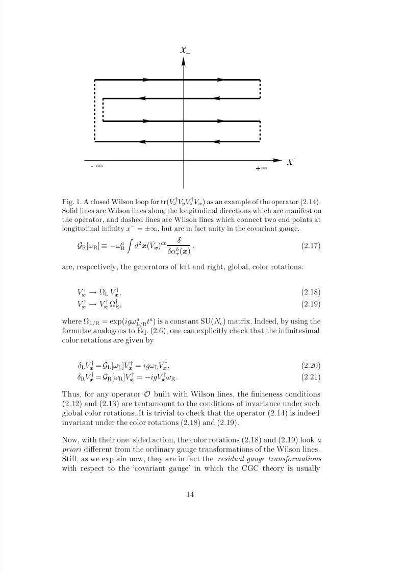
The operator (2.14) which has been seen to obey an infrared–finite evolutionequation is the covariant–gauge expression of a gauge invariant operator. In-deed, one can rewrite this operator as the trace of a closed Wilson loop, forwhich gauge symmetry is manifest. To that aim, note that the end points atlongitudinal infinity (x− = ±∞) of two adjacent Wilson lines (say, V †xi and V yi)can be connected by a Wilson line in the transverse direction, which is simplyunity in the present gauge, in which Ai

a = 0. Therefore, one can connect theend points of all the Wilson lines which enter the trace in Eq. (2.14) can beconnected in such a way to form a single, closed, Wilson loop (see Figure 1).

This observation suggests that there is an intimate relation between the in-frared finiteness and gauge invariance, that we would like to clarify now. Tothis end, we first notice that the differential operators which enter the finite-ness conditions, namely

GL[ωL] ≡ ωaL

d2x

δ

δαaτ (x)

, (2.16)

13



x+

-

x

-

Fig. 1. A closed Wilson loop for tr(V †x V yV †z V w) as an example of the operator (2.14).Solid lines are Wilson lines along the longitudinal directions which are manifest onthe operator, and dashed lines are Wilson lines which connect two end points atlongitudinal infinity x− = ±∞, but are in fact unity in the covariant gauge.

GR[ωR] ≡ −ωaR

d2x( V x)ab

δ

δαbτ (x)

, (2.17)

are, respectively, the generators of left and right, global, color rotations:

V †x

→ΩL V †x, (2.18)

V †x → V †x Ω†R, (2.19)

where ΩL/R = exp(igωaL/Rta) is a constant SU(N c) matrix. Indeed, by using the

formulae analogous to Eq. (2.6), one can explicitly check that the infinitesimalcolor rotations are given by

δLV †x = GL[ωL]V †x = igωLV †x , (2.20)

δRV †x = GR[ωR]V †x = −igV †xωR. (2.21)

Thus, for any operator

Obuilt with Wilson lines, the finiteness conditions

(2.12) and (2.13) are tantamount to the conditions of invariance under suchglobal color rotations. It is trivial to check that the operator (2.14) is indeedinvariant under the color rotations (2.18) and (2.19).

Now, with their one–sided action, the color rotations (2.18) and (2.19) look a

priori different from the ordinary gauge transformations of the Wilson lines.Still, as we explain now, they are in fact the residual gauge transformations

with respect to the ‘covariant gauge’ in which the CGC theory is usually

14



formulated (see [31] for details). We recall here that, in this gauge, the vectorpotential has only one non–zero component, the light–cone field A+

a ≡ αa,which is independent of x+. This structure of the field is preserved by a gaugetransformation Aµ → Ω(Aµ + i

g∂ µ)Ω† in which the gauge function Ω depends

only upon x−. Thus a residual gauge transformation amounts to

A+ → Ω(x−)

A+ +

i

g∂ +

Ω†(x−), Ω(x−) = eigω

a(x−)ta , (2.22)

which induces the following transformation for the Wilson line V †x :

V †x → Ω(x− = ∞) V †x Ω†(x− = −∞). (2.23)

So far, the gauge function ω(x−) is arbitrary. The ”global” color rotationsintroduced in Eqs. (2.18) and (2.19) are now obtained as the two (independent)special gauge transformations in which ω(x−) → 0 (and thus Ω(x−) → 1) ateither x− → −∞ (for the left rotation (2.18)) or x− → +∞ (for the rightrotation (2.19)). This establishes the interpretation of the finiteness conditionsas the conditions for gauge symmetry 4 .

Finally, let us show the infinitesimal transformation for the gauge field inte-grated over the longitudinal direction: αa(x) =

dx−αa(x−,x). As we will

discuss shortly, this is a natural variable in the weak–field regime. SinceA+ = α(x−,x) transforms as in Eq. (2.22), its infinitesimal change is given by

δα(x−

,x) = ∂ +

ω(x−

). Therefore, αa

(x) transforms as

αa(x) −→ αa(x) +

∞ −∞

dx−∂ +ωa(x−) = αa(x) + ξa, (2.24)

with ξa ≡ ωa(x− = ∞) − ωa(x− = −∞) being a pure number. This transfor-mation law will be useful in checking the gauge invariance of various operatorsin the weak–field limit.

4 Note also that the left and right generators form two independent SU(N c) algebra,as is expected for gauge transformations. More precisely, the differential operatorsJ aL(x) ≡ − 1

igδ

δαax

, and J aR(x) ≡ 1ig (V x)ab δ

δαbx

, which enter the definitions of the left

and right generators, satisfy the following algebra [δxy ≡ δ(2)(x− y)]

[J aL(x), J bL(y)] = if abcJ cL(x)δxy , [J aR(x), J bR(y)] = if abcJ cR(x)δxy ,

and commute with each other [J aL(x), J bR(y)] = 0.

15



3 Weak–field regime and Green’s functions in the CGC

In order to make contact with previous evolution equations proposed in per-turbative QCD at high energy, like the BFKL [1] and BKP [4,5] equations,

which neglect saturation effects and therefore apply only in the dilute regimeat relatively high transverse momenta (well above the saturation scale), itis convenient to consider also the weak–field limit of the JIMWLK equation(here, with dipolar kernel). When gα ≪ 1, one can expand the Wilson linesin Eq. (2.3) to lowest nontrivial order, to obtain

(1 − V †z V x)fa ≈ ig(αc(x) − αc(z))(T c)fa, (3.1)

where

αa(x) ≡ dx− αa(x−,x) ≡ αax (3.2)

is the effective color field in the transverse plane, as obtained after integratingover the longitudinal profile of the hadron. Then, the kernel η becomes simplyquadratic in αa

x, and the evolution equation (2.11) reduces to

∂

∂τ Oτ = g2

16π3

xyz

(x− y)2

(x− z)2(z − y)2

×(αx − αz)a(αy − αz)bf acf f bfd δδαcτ (x) δδαd

τ (y)Oτ

.(3.3)

For consistency with the above manipulations, the observable O — whichin general is some operator built with Wilson lines (see, e.g., Eq. (2.14)) —must be correspondingly expanded in powers of gα. Note that the relevantorder for this expansion depends upon the operator at hand, and also uponthe channel that we consider for scattering (see Sect. 4). For instance, forthe dipole operator shown in Eq. (2.8), the lowest nontrivial contribution isobtained after expanding the Wilson lines up to second order in gα :

V †x [α] ≈ 1 + ig

dx−αa(x−,x)ta (3.4)

− g2

2

dx−

dy−αa(x−,x)αb(y−,x)[θ(x− − y−)tatb + θ(y− − x−)tbta].

Clearly, to this order, the ordering of the color matrices αa(x−,x)ta in x− startsto play a role in the expansion of the Wilson lines. But this ordering is stillirrelevant for the computation of the dipole S –matrix to lowest order, because

16



of the symmetry of the color trace in Eq. (2.8) : tr(tatb) = 12

δab = tr(tbta).Namely, one finds:

S (x,y; α)≡

1

N ctr(V †xV y)

≃1

−g2

4N c(αa

x

−αay)2, (3.5)

where the final expression involves only the two–dimensional field αax, cf.

Eq. (3.2). The latter property turns out to be shared by all the operatorsfor weak (single) scattering that we shall discuss throughout this work. Thisfeature, together with the structure of the simplified evolution Hamiltonianmanifest on Eq. (3.3), enable us to consider the weak field approximation tothe CGC effective theory as being restricted to the Hilbert space of the func-tions built with αa

x. Onto this space, the functional derivatives in Eq. (3.3) canbe trivially replaced by δ/δαa

x. Thus, in this approximation, the longitudinal

structure of the color field becomes irrelevant.

Note that the weak–field Hamiltonian in Eq. (3.3) is quadratic both in αand in the functional derivative with respect to α. Thus, when acting on then–point function α(x1)α(x2) · · · α(xn)τ , this Hamiltonian does not changethe number n of fields. This has an important consequence for the weak–fieldevolution described by Eq. (3.3): During this evolution, the number of gluonsin the t-channel remains fixed , familiar to the ‘multi–reggeons’ approachesbased on BFKL evolution [7,4,5,8,10], to which we shall eventually comparethe present formalism. In particular, this implies that the JIMWLK evolutionin the weak–field regime is linear .

It is already known [32,33] that, in the weak field limit, the JIMWLK evolutionof the dipole S –matrix reduces to the corresponding BFKL equation [1]. Thiscan be easily checked on the first Balitsky equation, Eq. (2.9), by first rewritingthis equation in terms of the dipole scattering amplitude,

− iT (x,y; α) ≡ 1 − S (x,y; α) = 1 − 1

N ctr(V †xV y) , (3.6)

and then linearizing the ensuing equation with respect to T , which is formally 5

appropriate in the weak scattering regime where |T | ≪ 1. But for the followingdevelopments in this paper it is still instructive to give a rapid derivation of theBFKL equation, by using directly the weak field approximation in Eqs. (3.3)and (3.5). Specifically, in this approximation −iT (x,y)τ ≃ N (x,y)τ , with:

5 We ignore here the subtleties associated with fluctuations in the dilute regimewhich in general render such a linearization illegitimate even when |T τ | ≪ 1; seeRef. [16] for details.

17



N (x,y)τ ≃ g2

4N c(αa

x − αay)2τ

≡ g2

4N c[f τ (x,x) + f τ (y,y) − 2f τ (x,y)] , (3.7)

with the following definition for the 2–point Green’s function of the color fieldsin the dilute regime:

f τ (x,y) ≡ αa(x)αa(y)τ = f τ (y,x). (3.8)

Note that, although colorless (it carries no open color indices), the object inEq. (3.8) is still not gauge invariant: the residual gauge transformation for αa

x

consists in the constant shift αax → αa

x + ξa [cf. Eq. (2.24)], but f τ (x,y) isnot invariant under this operation. On the other hand, the linear combinationyielding the scattering amplitude (3.7) is clearly invariant, as it should (since

Eq. (3.7) has been obtained after a consistent expansion of the gauge–invariantoperator (3.6)). Thus, a priori , one is allowed to use the dipolar form of theevolution equation, Eq. (3.3), for the physical amplitude (αa

x − αay)2τ , but

not also for the Green’s function f τ (x,y). Still, since Eq. (3.3) is linear in O,it is clear that the equation obeyed by (αa

x − αay)2τ is correctly obtained by

separately evolving each of the Green’s functions in the second line of Eq. (3.7),and then summing up the corresponding results. This argument shows that,in fact, it is legitimate to use the dipolar evolution equation (3.3) even forquantities which by themselves are not gauge invariant, so like the Green’sfunction (3.8), provided these quantities are eventually used as building blocksin the construction of gauge–invariant observables. In such a case, the use

of the dipolar Hamiltonian H dp can be seen as a convenient prescription toregulate the infrared singularities which would appear at intermediate stepswhen using the original JIMWLK Hamiltonian in Eqs. (2.2)–(2.3).

Specifically, by using Eq. (3.3) for O = αaxαa

y, one easily finds

∂

∂τ f τ (x,y) =

αs

2π

d2z

(x− y)2

(x− z)2(y − z)2(3.9)

×

f τ (x, z) + f τ (y, z) − f τ (x,y) − f τ (z, z)

.

This equation is well defined both in the infrared (because of the rapid decayof the dipole kernel at large values of z), and in the ultraviolet (the short–distance poles of the kernel at x = z and y = z are actually harmless becausethey have zero residue). By contrast, the equation which is obtained by actingon αa

xαay with the (weak–field version of the) original JIMWLK Hamiltonian 6

contains terms which are potentially singular at large distances.

6 This equation can be found, e.g., as Eq. (3.10) in Ref. [45].

18



By using Eqs. (3.7) and (3.9), one finds the coordinate space (or ‘dipolar’)version of the BFKL equation for N (x,y)τ , as expected:

∂ ∂τ

N (x,y)τ = αs

2π d2z (x− y)

2

(x− z)2(y − z)2(3.10)

×N (x, z)τ + N (z,y)τ − N (x,y)τ

.

In this last equation, ultraviolet finiteness is ensured by the vanishing of thescattering amplitude at equal points, N (x,x) = 0, a property consistentwith Eq. (3.7) and which reflects ‘color transparency’.

In what follows, we shall take Eq. (3.9) (supplemented with an appropri-

ate initial condition) as the definition of the 2–point Green’s function in theCGC formalism. This situation illustrates a general feature of the presentapproach, namely the fact that, because of infrared complications, the defi-nition of Green’s functions meets with ambiguities which disappear only inthe construction of gauge–invariant quantities. Of course, these Green’s func-tions are only intermediate objects, which are strictly speaking not needed:it is always possible to construct directly the equation obeyed by the gauge–invariant quantity of interest, which is then free of any ambiguity. The reasonwhy it is nevertheless convenient to introduce such Green’s functions, it isbecause these are the CGC analogs of the multi–gluon exchanges consideredin the more traditional approaches to high energy QCD [7,4,5,8,10], to which

we would like to establish a connection in the forthcoming sections.

4 Odderon operators in the CGC

With this section, we start our discussion of the odderon within the CGC

framework. To start with, we shall construct the operators describing multi-ple odderon exchanges in the scattering between the CGC and a relativelysimple projectile, such as a color dipole, or three quarks in a colorless state.The dipole–CGC scattering can be viewed as a sub–process of the diffractivescattering of a virtual photon on some dense hadronic target (the CGC), aprocess in which odderon contributions are expected, e.g., in the productionof C –even mesons like ηc (see, e.g., [12,46]). As for the 3–quark system, thismay be viewed as a crude ‘valence quark’ model of the baryon.

19



4.1 The dipole-CGC scattering

Consider first the simplest case, namely the high energy scattering of a qqdipole off the CGC, and let us briefly outline the construction of the cor-

responding S –matrix. As explained in Sect. 2.1, we need to first computethe S –matrix for a fixed configuration of the classical field α, and then aver-age over the latter. For the first step, we can use the eikonal approximation:S (x,y; α) = out|in, where the transverse positions of the quark (x) and theantiquark (y) are the same in the in–coming and the out–going states. Onecan write, schematically, (i = 1, · · · , N c is the color index)

| in ∼ ψini (x)ψin

i (y) |0 , | out ∼ ψouti (x)ψout

i (y) |0 ,

where the appropriate normalization is understood. The relation between the

in–coming and the out–going fields is found by solving (the high–energy ver-sion of) the Dirac equation (∂ − − igαata)ψ = 0 for a given gauge field con-figuration α. This implies that ψout

i = (V †x)ijψin j with the Wilson line in the

fundamental representation. The S -matrix becomes:

S (x,y; α) = out|in =1

N c(V †x)ij(V y)kiδklδ jl =

1

N ctr(V †xV y),

(we have restored the appropriate normalization), in agreement with Eq. (2.8).The physical S –matrix is finally obtained after averaging over the randomclassical color field, cf. Eq. (2.1), an operation which also introduces the de-pendence upon the energy (i.e., upon τ ):

S τ (x,y) =1

N ctr(V †xV y)τ . (4.1)

Since non–linear in α, the above formula describes in general multiple ex-changes, which can be either even, or odd, under the operation of chargeconjugation C . To single out C –even (‘pomeron’) or C –odd (‘odderon’) ex-changes, one needs to project Eq. (4.1) onto incoming and outgoing stateswith appropriate C –parities. Since the charge conjugation for fermions is de-

fined by CψC −1 = −i(ψγ 0γ 2)T , and C ψC −1 = (−iγ 0γ 2ψ)T , it is clear that theeigenstates of C in the dipole sector are given by (ψ(x)ψ(y) ± ψ(y)ψ(x)) |0,where +(−) sign yields the C -even(odd) state. These structures are naturalbecause the charge conjugation is essentially the exchange of a quark and anantiquark.

Taking the C –odd dipole state as the in–coming state (this is the state selectedby the virtual photon wavefunction), and the C –even dipole state as the out–

20



going state (this would be selected by a ηc meson), one obtains the followingC –odd contribution to the S -matrix:

S odd(x,y) = out, even | in, odd =1

2N c tr(V †xV y) − tr(V †yV x)

τ . (4.2)

This allows us to identify the operator for C –odd exchanges in the dipole–CGCscattering (”the dipole odderon operator”) as

O(x,y) ≡ 1

2iN ctr(V †xV y − V †yV x) = − O(y,x), (4.3)

where the factor of i is introduced in order for this quantity to be real: indeed,since V and V † are unitary matrices, we have [tr(V †xV y)]∗ = tr(V †yV x).

One can directly check, by using the transformation property of the gaugefields under charge conjugation,

C Aµ C −1 = −(Aµ)T , (4.4)

that the operator (4.3) is indeed C –odd: For a generic Wilson line V con-structed with Aµ, Eq. (4.4) implies

C V C −1 = (V †)T = V ∗, (4.5)

so that C tr(V †xV y) C −1 = tr(V †yV x), or, finally, C O(x,y) C −1 = −O(x,y).

Note that the C –odd contribution (4.2) is the imaginary part of the S –matrixelement, or, equivalently, the real part of the scattering amplitude T , withS = 1 + iT :

O(x,y)τ = ℑm S τ (x,y), (4.6)

which was to be expected. Correspondingly, the C –even, Pomeron exchange,amplitude, that we shall denote as N (x,y), is identified with the real part of

the S -matrix:

N (x,y) ≡ 1 − 1

2N ctr(V †xV y + V †yV x), (4.7)

N (x,y)τ = 1 − ℜe S τ (x,y). (4.8)

Operatorially, S = 1+iT = 1−N +iO. Note the obvious boundary conditionswhich follow from S τ (x,x) = 1 (or directly from the definitions (4.3), (4.7)):

21



N (x,x) = O(x,x) = 0. (4.9)

Clearly, these conditions remain true after averaging over the random field α.

From perturbative QCD, we expect the lowest order contribution to the odd-eron exchange to be represented by three gluons tied up together with thedabc symbol, where dabc = 2tr(ta, tbtc) is the totally symmetric tensor. Theoperator dabcAa

µ(x)Abν (y)Ac

ρ(z) is indeed C –odd, as obvious from Eq. (4.4).Let us check that a similar structure emerges also from the CGC operator(4.3) when this is evaluated in the weak–field limit. The lowest non–trivialcontribution to Eq. (4.3) is obtained by expanding the Wilson lines there upto cubic order in the field α in the exponent. (The terms quadratic in α cancelin the difference of traces in Eq. (4.3).) By collecting the remaining terms, oneobtains:

O(x,y) ≃ −g3

24N c dabc 3(α

axα

byα

cy − α

axα

bxα

cy) + (α

axα

bxα

cx − α

ayα

byα

cy) .(4.10)

As expected, this expression is cubic in αa with the color indices contractedsymmetrically by the d–symbol. Note that, because of the symmetry propertiesof this symbol, the path–ordering of the Wilson lines in x− has been irrelevantfor computing O(x,y).

The linear combination of trilinear field operators in Eq. (4.10) is gauge invari-ant by construction. To render this more explicit, let us rewrite this operatoras

O(x,y) ≃ −g3

24N cdabc(αa

x − αay)(αb

x − αby)(αc

x − αcy). (4.11)

This is manifestly invariant under a residual gauge transformation, which con-sists in a constant shift of the field: αa → αa + ξa (cf. Eq. (2.24)). In fact, analternative way to construct the gauge–invariant linear combination appear-ing in Eq. (4.10) is to directly impose the (weak-field version of the) finitenessconditions (2.12) and (2.13) on the C –odd Green’s function dabcαa

xαbyαc

yτ .

4.2 The 3-quark–CGC scattering

To describe the 3–quark colorless state, we shall use the following ”baryonic”operator 7 ǫijkψi(x)ψ j(y)ψk(z), where ǫijk is the complete antisymmetric sym-bol, and the color indices i,j,k can take the values 1,2, or 3. Thus, the con-struction below applies only for N c = 3. (The generalization to arbitrary N c

7 A similar approach was adopted for the proton-proton scattering in Refs. [47,48].

22



is in principle possible, but the analysis becomes more complicated becausethe baryonic operator is then built with N c quark fields.) By using the sametechnique as for dipole–CGC scattering, one obtains the following S –matrix:

S τ (x,y, z) =1

3! ǫijkǫlmnV †il (x)V

† jm(y)V

†kn(z)τ , (4.12)

where x, y, and z are the transverse positions of the three quarks. This op-erator is symmetric under any permutations of the three coordinates, and isnormalized as S τ (x,x,x) = 1. By using Eq. (4.4), it is easy to check that theodderon contribution is given again by the imaginary part of the S -matrix :

B(x,y, z)τ = ℑm S τ (x,y, z), (4.13)

where the ”3–quark odderon operator” B(x,y, z) has been defined as

B(x,y, z) =1

3!2i

ǫijkǫlmnV †il (x)V † jm(y)V †kn(z) − c.c.

. (4.14)

This is totally symmetric too, and satisfies the boundary condition B(x,x,x) =0, which is an immediate consequence of the normalization S τ (x,x,x) = 1.

The simplest way to see that the operator (4.14) is gauge invariant is to noticethat this can be rewritten in terms of the manifestly gauge invariant operatorsshown in Eq. (2.14). Indeed, by using the identity 8

1

3!ǫijkǫlmnV il(w)V jm(w)V kn(w) = det V (w) = 1, (4.15)

where w is an arbitrary transverse coordinate, one can equivalently rewritethe 3–quark odderon operator B as

B(x,y, z) =1

3!2i

tr(V †xV w)tr(V †yV w)tr(V †zV w) − tr(V †xV w)tr(V †yV wV †zV w)

−tr(V †yV w)tr(V †xV wV †zV w)

−tr(V †zV w)tr(V †xV wV †yV w)

+tr(V †xV wV †yV wV †zV w) + tr(V †xV wV †zV wV †yV w) − c.c. . (4.16)

Note that this expression involves not only dipolar operators, but also highermulti-polar ones (quadrupoles and sextupoles). By construction, this expres-sion is independent off w when N c = 3. Thus, it can be simplified by choosing

8 We have already used a similar relation when we have specified the normalizationof S τ (x,y,z).

23



w to be one of the quark coordinates, say w = z. Then, Eq. (4.16) reducesto:

B(x,y, z) =1

3!2itr(V †xV z)tr(V †yV z)

−tr(V †xV zV †yV z)

−c.c.. (4.17)

which looks indeed considerably simpler, but where the symmetry in x, y andz is not manifest anymore (although, for N c = 3, we know that this expressionis totally symmetric, by construction).

In particular, when two of the coordinates are the same, the 3–quark odderonoperator reduces to the dipole odderon operator, Eq. (4.3):

B(x, z, z) = O(x, z) =−

B(x,x, z). (N c = 3) (4.18)

This is physically reasonable, because the diquark state is equivalent to anantiquark as far as color degrees of freedom are concerned, and can be mosteasily checked by setting y = z in the r.h.s. of Eq. (4.17). Note however that,if one rather sets y = x in the same expression, then it is not immediatelyobvious that the ensuing expression for B(x,x, z) is indeed equal to −O(x, z)when N c = 3, as it should. This is so because of the lack of manifest symmetryof Eq. (4.17), as alluded to above. Still, by diagonalizing the unitary matrixV †x V z, and after performing some simple algebraic manipulations (relying onthe fact that the corresponding eigenvalues λi, i = 1, 2, 3, are pure phases

and obey λ1λ2λ3 = 1), it is possible to check that the equality B(x,x,z) =−O(x, z) = −B(x, z, z) holds indeed.

In the weak field approximation, as obtained after expanding to lowest non–trivial order (i.e., to cubic order in α) the Wilson lines in any of the previousexpressions for B(x,y, z), one finds again a gauge invariant linear combinationof trilinear field operators with the color indices contracted with the d–symbol:

B(x,y, z)

≃g3

144

dabc (4.19)

×(αa

x − αaz) + (αa

y − αaz)

(αby − αb

x) + (αbz − αb

x)

(αcz − αc

y) + (αcx − αc

y)

.

In fact, in this weak–field regime, the 3–quark C –odd operator is fully de-termined by gauge symmetry together with the requirement of total symme-try with respect to the external coordinates: Indeed, it can be checked thatEq. (4.19) uniquely emerges from the C –odd Green’s function (5.1) after sym-metrization and imposing the finiteness condition (2.12).

24



5 Odderon evolution in the dipole–CGC scattering

In this and the next sections, we shall apply the general JIMWLK equation (inits dipolar form, cf. Eq. (2.11)) to the operators describing odderon exchanges

constructed in the previous section, in order to deduce the evolution equationsfor the respective, C –odd, scattering amplitudes.

We start with the simpler case of the dipole scattering, for which we shalldiscuss separately the weak–field limit (corresponding to a single scattering),and the general, non–linear, case (which includes multiple scattering). In fact,in this particular case, it is rather straightforward to write down directly thenon–linear equations (see below), from which the equations for the weak–fieldlimit can be then simply deduced by linearization. Still, the more detailedapproach that we shall follow below is instructive as a preparation for themore tedious case of the 3–quark operator, to be discussed in Sect. 6.

5.1 Linear evolution and the odderon Green’s function

In the weak–field regime, where we can limit ourselves to a single odderonexchange, it is convenient to proceed as in Sect. 3 and introduce the (totallysymmetric) odderon Green’s function

f τ (x,y, z) ≡ dabcαaxαb

yαczτ , (5.1)

in terms of which the weak–field version of the dipole odderon operator (4.10)can be rewritten in a form similar to Eq. (3.7) for the pomeron:

O(x,y) ≃ −g3

24N c

3

f τ (x,y,y) − f τ (x,x,y)

+ f τ (x,x,x) − f τ (y,y,y)

.

(5.2)

The discussion of the pomeron Green’s function (3.8) in Sect. 3 applies to theodderon Green’s function (5.1) as well: The latter is not a gauge–invariantquantity, so its evolution under the original JIMWLK Hamiltonian would be

afflicted by infrared singularities, which can however be regulated by using the(weak field version of the) dipolar Hamiltonian H dp. This yields a mathemat-ically well defined equation for f τ (x,y, z), that we shall use as the definition

of the odderon Green’s function.

Still as in the pomeron case, the equation obeyed by the scattering amplitude(5.2) — which is gauge–invariant — is not sensitive to the ambiguities whichaffect the definition of the Green’s function, and comes out the same whatever

25



form of the Hamiltonian is used in its derivation. In fact, the only reason forintroducing the Green’s function (5.1) is the fact that it is for this functionthat we shall verify the BKP equation later on.

Specifically, by using Eq. (3.3) for O = dabcαaxαb

yαcz, and after some lengthy

algebra, one obtains

∂

∂τ f τ (x,y, z) =

αs

4π

d2w

(x− y)2

(x−w)2(y −w)2f τ (x,w, z) + f τ (w,y, z) − f τ (x,y, z) − f τ (w,w, z)

+

2 cyclic permutations

, (5.3)

which is like applying the equation (3.9) for the 2–point Green’s function toeach pair of points within f τ (x,y, z). It can be checked as before that this

equation is well defined both in the infrared and in the ultraviolet. It is nowstraightforward to construct the equation obeyed by the linear combinationin Eq. (5.2), and thus find that this is precisely the BFKL equation (3.10)

∂

∂τ O(x,y)τ = αs

2π

d2z

(x− y)2

(x− z)2(y − z)2

×O(x, z)τ + O(z,y)τ − O(x,y)τ

(5.4)

(we have also used the identity f eagf dbgdabc = N c2

dedc), in agreement with anoriginal observation by Kovchegov, Szymanowski and Wallon [43]. In view

of the formal difference between the pomeron and the odderon operators, asgiven by Eqs. (3.7) and, respectively, (4.10), it may appear as a surprise thatthey obey both the same evolution equation. But this becomes more naturalif one remembers that N and O are, respectively, the imaginary part and thereal part of the scattering amplitude T (with S = 1+iT ), and that in the weakfield regime T obeys a linear equation with real coefficients — the linearizedversion of the first Balitsky equation, Eq. (2.9) — which is therefore separatelysatisfied by its real and imaginary parts.

But since the initial conditions corresponding to N and O are different (inparticular, they have different C –parities), so are also the respective solutions,and their behaviors at high energy. In Appendix A, we compute within theCGC formalism the C –odd initial conditions for some simple targets: a barequark and a qq dipole. Namely, if the target is a single quark with transverseposition x0, one obtains

O(x,y)τ =0 =α3s

12

(N 2c − 4)(N 2c − 1)

N 3cln3 |x− x0|

|y − x0| , (5.5)

26



whereas for the more interesting case of a dipolar target (with the quark beingat x0 and the antiquark at y0), one rather finds

O(x,y)τ =0 =

α3s

12

(N 2c−

4)(N 2c−

1)

N 3c ln3

|x

−x0

||y

−y0

||x− y0||y − x0| . (5.6)

These expressions are in agreement with the corresponding results in Ref. [43]up to an overall numerical factor. As expected, these initial conditions areantisymmetric under the exchange of x and y, and thus satisfy the boundarycondition (4.9). It is easily checked that this boundary condition is preservedby the evolution according to Eq. (5.4), as necessary for this equation to bewell defined.

The high–energy behavior of the odderon solution to Eq. (5.4) has been an-

alyzed too in Ref. [43], where it has been shown that the projection of thegeneral BFKL solution onto C –odd initial conditions selects (C –odd) BFKLeigenfunctions whose maximal intercept is equal to one. It turns out that theseare the same eigenfunctions that were previously identified, by Bartels, Lipa-tov, and Vacca [12], as exact solutions to the momentum–space BKP equation[4,5]. Thus, in contrast to the pomeron solution to the BFKL equation, whichat high energy rises exponentially with Y ( N (Y ) ∼ e(αP−1)Y , with the BFKLintercept αP = 1 + (4 ln 2)αsN c/π [1]), the corresponding odderon solutionrises only slowly, as a power of Y ∼ ln s.

But, of course, these types of high–energy behavior (for either N or O), whichare mathematical consequences of the BFKL equation, are physically accept-able only so far as this equation is a correct approximation, that is, withinthe limited range of energies where the unitarity corrections are indeed neg-ligible. For higher energies, the evolution is governed by more complicated,non–linear, equations, to which we now turn.

5.2 Non–Linear evolution

For dipole–CGC scattering, the general evolution equations obeyed by theaverage amplitudes N (x,y)τ and O(x,y)τ in the strong field regime canbe easily inferred from the first Balitsky equation (2.9) : Since the operatorsN (x,y) and O(x,y) are, respectively, the real part and the imaginary part of the dipole S –matrix S (x,y) = (1/N c)tr(V †xV y), cf. Eqs. (4.3) and (4.7), it isclear that the respective equations can be simply obtained by separating thereal part and the imaginary part in Eq. (2.9). One thus obtain:

27



∂


2π

d2z

(x− y)2

(x− z)2(z − y)2

×

O(x, z) + O(z,y) − O(x,y)

− O(x, z)N (z,y) − N (x, z)O(z,y)

τ , (5.7)

∂ ∂τ

N (x,y)τ = αs

2π

d2z (x− y)2

(x− z)2(z − y)2

×

N (x, z) + N (z,y) − N (x,y)

− N (x, z)N (z,y) + O(x, z)O(z,y)τ

. (5.8)

As is generally the case for the Balitsky equations, the equations above do notclose by themselves, but rather belong to an infinite hierarchy. Interestingly,the non–linear terms in these equations couple the evolution of C –odd andC –even operators. For instance, the last term, quadratic in O, in the r.h.s. of Eq. (5.8) for N τ describes the merging of two odderons into one pomeron.This process has not been recognized in previous studies of the Balitsky hi-erarchy, but the vertex connecting one pomeron to two odderons has beenalready computed in lowest order perturbation theory [26], and it would beinteresting to compare such previous results with the corresponding vertex inEq. (5.8) (which is essentially the dipole kernel).

But the odderon–pomeron coupling which turns out to have the most dramaticconsequences is the one encoded in the last terms in Eq. (5.7) for Oτ : Aswe shall shortly argue, this coupling leads to a rather rapid suppression of the

C –odd contributions to scattering in the high energy regime where unitaritycorrections start to be important (i.e., where N τ ∼ O(1)). To construct theargument without having to resort to an infinite hierarchy of equations, weshall restrict ourselves to the mean field approximation in which the non–linear terms in Eqs. (5.7)–(5.8) are assumed to factorize. In the strong fieldregime, which will be our main focus below, we expect this approximation tobe qualitatively correct [40].

In this mean field approximation, Eqs. (5.7)–(5.8) reduce to a closed systemof coupled, non–linear, equations for N τ and Oτ :

∂


2π

d2z

(x− y)2

(x− z)2(z − y)2(5.9)

×O(x, z)τ + O(z,y)τ − O(x,y)τ −O(x, z)τ N (z,y)τ − N (x, z)τ O(z,y)τ

,

28



∂

∂τ N (x,y)τ = αs

2π

d2z

(x− y)2

(x− z)2(z − y)2(5.10)

×N (x, z)τ + N (z,y)τ − N (x,y)τ −N (x, z)τ N (z,y)τ + O(x, z)τ O(z,y)τ

.

The first of these equations has been already proposed in Ref. [43], as aplausible non–linear generalization of Eq. (5.4). As for Eq. (5.10), this is theKovchegov equation [39] supplemented by a new term describing the mergingof two odderons.

The Kovchegov equation has been extensively studied over the last few years,both analytically and numerically, and although the exact solution is notknown, its general properties are by now well understood [49,50,51,52,53,54,55,56,57,58,59].In its most synthetic description, due to Munier and Peschansky [59] (see also[50]), this solution can be viewed as a front connecting the saturation regime

where 9 N = 1 — this is reached for dipole sizes r = |x − y| much largerthan the saturation length 1/Qs(τ ) — to the unstable regime at r ≪ 1/Qs(τ ),where the amplitude is small (N ≪ 1), but it rises rapidly with τ , according toBFKL equation. When increasing τ , the front propagates towards smaller val-ues of r (or larger transverse momenta), and its instantaneous position definesthe saturation momentum Qs(τ ). The latter is found to rise exponentially withτ : Q2

s(τ ) = Q20 ecαsτ , with c a numerical constant determined by the BFKL

dynamics [17,56,57,58].

As we shall argue below, this mean–field picture of the pomeron exchangesis not significantly modified by the odderon contribution to Eq. (5.10). In

particular, the values N = 1 and N = 0 remain as (stable and, respectively,unstable) fixed points of the evolution described by Eqs. (5.9)–(5.10), but tothem one should add a new fixed point, namely O = 0, which is asymptoticallyapproached at high energy.

It is first easy to check that N = 1 and O = 0 are indeed fixed points at highenergy. To also see that this is the only combination of fixed points in thislimit, notice from Eq. (5.9) that, when increasing N , the non–linear terms inthis equation act towards suppressing the odderon [43]. It is thus consistentto assume that, at high energy, the odderon contribution represents only a

small perturbation to the Kovchegov equation, so that the pomeron saturatesin the standard way: N (r, τ ) ≃ 1 for r ≫ 1/Qs(τ ). Also, the dominant energybehavior of the saturation momentum, i.e., the value of the saturation expo-nent c, should not change, since this is fully determined by the linear (BFKL)part of the equation for N . Using this assumption, it is possible to study theapproach of O towards zero, and thus check the consistency of our hypothesis.

9 Until the end of this section, we shall mostly use the simplified notations N andO for the respective expectation values.

29



Namely, for sufficiently high energy, such that r ≫ 1/Qs(τ ), the integral in ther.h.s. of Eq. (5.9) is dominated by relatively large dipoles, for which N ≃ 1.In this regime, the non–linear terms in this equation precisely cancel the firsttwo linear terms there, and the equation simplifies to

∂

∂τ O(x,y)τ ≃ −αs

r2 Q−2s (τ )

dz2

z2O(x,y)τ = −αs ln[Q2

s(τ )r2] O(x,y)τ , (5.11)

which together with ln[Q2s(τ )r2] = cαs(τ − τ 0) immediately implies:

O(x,y)τ ≃ exp− c

2α2s(τ − τ 0)2

O(x,y)τ 0 for r ≫ 1/Qs(τ ). (5.12)

As anticipated, this is a rapidly decreasing function of τ , which is actually

the same as the function describing the approach of the real part of the S –matrix towards the ‘black–disk’ limit S = 0 (the Levin-Tuchin law) [49,37].We expect the fluctuations neglected in the mean field approximation leadingto Eqs. (5.9)–(5.10) to modify (actually, decrease) the value of the overallcoefficient in the exponent of Eq. (5.12), but preserve the above qualitativepicture [40].

6 Odderon evolution in the scattering of the 3–quark system

The new feature which makes the 3–quark system conceptually interesting isthe fact that the corresponding scattering amplitude depends upon three inde-pendent transverse coordinates. Therefore, already the lowest–order odderonamplitude, as given in Eq. (4.19), involves configurations in which the threeexchanged gluons are attached to different quark legs, and which are thusprobing the complete functional dependence of the odderon Green’s functiondefined in Eq. (5.1). As we shall further argue in Sect. 7, this in turns impliesthat the 3–quark—CGC scattering is a good theoretical laboratory to studythe general solution to the BKP equation.

Our discussion in this section will be restricted to the weak–field version of the 3–quark odderon operator, Eq. (4.19), which describes scattering via theexchange of a single odderon. This is indeed sufficient to discuss the cor-respondence with the BKP equation in the next section. Within the CGCformalism, there is no difficulty of principle (other than the tediousness of thecorresponding algebraic manipulations) which would prevent us from derivingthe evolution equations satisfied by the general, non–linear, 3–quark opera-tors in Eqs. (4.14) or (4.16). However, these general equations are complicated

30



and not very illuminating: Through their non–linear terms, they couple the3–quark operator to other color structures. This is especially manifest if oneuses the form (4.16) of the 3–quark amplitude: this involves operators of var-ious multi-polar orders, which in the Balitsky hierarchy are coupled to otheroperators of even higher multi-polar moments.

By using the expression of B(x,y, z) as a linear combination of odderonGreen’s functions, as manifest in Eq. (4.19), together with the equation (5.3)obeyed by the latter, one can deduce after a straightforward but lengthy cal-culation the following linear evolution equation for Bxyzτ ≡ B(x,y, z)τ :

∂

∂τ Bxyzτ = 3αs

4π2

d2w

(x− y)2

(x−w)2(y −w)2

×Bxwzτ + Bwyzτ − Bxyzτ

−Bwwzτ − Bxxwτ − Byywτ − Bxywτ + (2 cyclic permutations). (6.1)

(Of course, the same equation could be obtained also directly from Eq. (3.3)with O = Bxyz, but the corresponding manipulations would be even more te-dious; the introduction of the Green’s function (5.1) at intermediate steps hasalso the advantage to better organize the calculation.) Note that Eq. (6.1) is aclosed equation for Bxyzτ , which was expected in view of gauge invariance:the only gauge invariant operators available are Bxyz and Oxy = Bxyy (cf.Eq. (4.18)).

Consider the structure of Eq. (6.1) in some detail: The linear combinationof B’s in the integrand vanishes at the points w = x and w = y where liethe poles of the dipole kernel, so the latter are again innocuous. Also, onecan easily check that the above equation is consistent with the relation (4.18)between the dipole and the 3–quark odderon amplitudes: if one sets z = y,Eq. (6.1) reduces indeed to Eq. (5.4) with N c = 3. Lastly, Eq. (6.1) manifestlypreserves the symmetry of the scattering amplitude under the permutation of its three coordinate variables.

The initial condition can be calculated within the CGC formalism, in a similarway as for dipole–CGC scattering (cf. Appendix A). For example, for a singlequark at transverse position x0, one finds

Bxyzτ =0 (6.2)

=5

34α3s ln

|x− x0||y − x0||z − x0|2

ln|y − x0||z − x0|

|x− x0|2ln

|z − x0||x− x0||y − x0|2

.

As expected, this is symmetric under the permutation of the three external

31



coordinates, and satisfies the boundary condition Bxxxτ = 0.

In the next section, we shall argue that the high energy behavior of the solu-tion Bxyzτ to Eq. (6.1) is controlled by the BLV solution [12] to the BKPequation, and thus has a maximal intercept equal to one.

7 Comparison with previous approaches

Within the traditional perturbative QCD approach to small–x evolution, theodderon exchange is viewed as the exchange of a composite object made of three reggeized gluons which evolves with energy according to the Bartels–Kwiecinski–Praszalowicz (BKP) equation [4,5]. From the point of view of theCGC formalism, this exchange is a single scattering, and should be comparedto the weak–field limit of the corresponding CGC equations, as derived in

the previous sections. In what follows, we shall demonstrate that the BKPodderon corresponds to the CGC Green’s function introduced in Eq. (5.1):The BKP equation, which is traditionally written in momentum space, isessentially the Fourier transform of Eq. (5.1) for f τ (x,y, z). Based on ourprevious discussion of gauge–invariant scattering amplitudes, we shall thenargue that the natural Hilbert space for discussing odderon exchanges is infact larger than the one which is generally used in the literature, and withinwhich the BFKL Hamiltonian shows holomorphic separability [8,10].

7.1 Relation to the BKP equation

The BKP equation is traditionally written in momentum space as

∂

∂τ F τ (k1,k2,k3) =

1

2

3i=1

d2k′1d2k′2d2k′3 δ(2)(k′1 + k′2 + k′3 − q) δ(2)(ki − k′i)

×H BFKL(ki−1,ki+1;k′i−1,k′i+1)F τ (k′1,k′2,k′3), (7.1)

where F τ (k1,k2,k3) is the Green’s function for the exchange of three reggeizedgluons (with transverse momenta k

1, k

2, and k

3, respectively) in a C –odd,

color singlet, state. Furthermore, k4 ≡ k1 (and similarly k′4 ≡ k′1), and q isthe momentum transfer. The factor 1

2 accounts for the fact that two of thegluons are in the color octet state. Finally, H BFKL is the non-forward BFKLkernel including the virtual terms:

H BFKL(k1,k2;k′1,k′2) =k2

1k′22 + k2

2k′21 − (k1 − k′1)2(k1 + k2)2

k21k

22(k1 − k′1)2

32



−πδ(2)(k′1 − k1)

lnk2

1

ǫ2+ ln

k22

ǫ2

, (7.2)

where ǫ is an infrared cutoff which does not affect physical results.

The function F τ (k1,k2,k3) is often referred to as a ‘scattering amplitude’, butin fact the physical amplitudes are obtained only after convoluting this withappropriate impact factors. A generic odderon amplitude reads:

O(q) =

d2k1d2k2d2k3 δ(2)(k1 + k2 + k3 − q)

× Φproj(k1,k2,k3) F τ (k1,k2,k3), (7.3)

where gauge symmetry requires the projectile impact factor Φproj(k1,k2,k3)to vanish when ki = 0 for some i (indeed, a zero–momentum gluon ‘sees’the projectile as a whole, and the latter is globally colorless). Note that, when

writing the scattering amplitude as in Eq. (7.3), the impact factor of the targetis implicitly included in the definition of F τ . This is in line with the generalapproach in this paper, where the target is a generic ‘color glass condensate’,and the CGC Green’s functions like those in Eqs. (3.8) or (5.1) include therelevant information about the target impact factor.

In the case where the projectile is a proton, the odderon impact factor isexpected in the form (see, e.g., [48])

Φproton(k1,k2,k3) = d2xd2yd2z

|Ψproton(x,y, z)

|2(2 eik1x

−eik1y

−eik1z)

×(2 eik2y − eik2z − eik2x)(2eik3z − eik3x − eik3y), (7.4)

where |Ψproton(x,y, z)|2 is the proton light–cone wavefunction, with x, y,and z denoting the coordinates of the three valence quarks relative to theirbarycenter. (The condition x + y + z = 0 is implicit in the definition of |Ψproton|2.) The exponential terms within the parentheses correspond to allthe possible attachments of the three exchanged gluons to the quark lines inthe proton. Note that Φproton(k1 = 0,k2,k3) = 0, etc., as expected.

Furthermore, if the projectile is a virtual photon, the odderon couples to the

dipole component of the photon Fock space, so that:

Φγ ∗(k1,k2,k3) =

dzd2r|Ψγ ∗(z, r)|2 (7.5)

×( eik1r2 − e−ik1

r2 )( eik2

r2 − e−ik2

r2 )( eik3

r2 − e−ik3

r2 ),

where r is the dipole size, and Ψγ ∗ is the light–cone wavefunction describingthe dissociation of the virtual photon, and can be computed in perturbation

33



theory with respect to αEM [60].

To make contact between this more traditional approach and our previousresults in this paper, it is convenient to introduce first the momentum spaceversion of the odderon Green’s function introduced in Eq. (5.1). We thus

define:

f τ (k1,k2,k3) ≡

d2xd2yd2z

(2π)6e−ik1x−ik2y−ik3z f τ (x,y, z) , (7.6)

in terms of which the scattering amplitudes O(x,y)τ and B(x,y, z)τ canbe rewritten as

O(x,y)τ = d2k1d2k2d2k3f τ (k1,k2,k3) (7.7)

×( eik1x − eik1y)( eik2x − eik2y)( eik3x − eik3y),

and, respectively,

B(x,y, z)τ =

d2k1d2k2d2k3 f τ (k1,k2,k3)(2eik1x − eik1y − eik1z)

×(2 eik2y − eik2z − eik2x)(2eik3z − eik3x − eik3y). (7.8)

Note the similarity between the exponential factors in these equations andthose in Eqs. (7.4) and (7.5) for the impact factors. This reflects the fact thatthe couplings between the exchanged gluons and the quarks (or antiquarks) inthe projectile have been explicitly included in our definition of the scatteringamplitudes. By inspection of the previous equations, it becomes clear thatthe CGC Green’s function f τ (k1,k2,k3) should correspond to the functionF τ (k1,k2,k3) of the traditional BKP approach. To be able to compare these

quantities, one also needs the equation satisfied by f τ (k1,k2,k3), which isobtained after taking a Fourier transform in Eq. (5.3). A lengthy but straight-forward calculation shows that the resulting equation is the same as the BKPequation (7.1) up to terms proportional to delta–functions δ(2)(ki) (i = 1, 2, 3),which are however irrelevant for the calculation of the scattering amplitudes,since they do not contribute to the convolutions in Eqs. (7.3) or (7.7)–(7.8).This demonstrates the equivalence between the two formalisms, in so far asthe single odderon exchanges are considered.

34



7.2 Comments on the Hilbert space for odderon solutions

Following the remarkable discovery by Lipatov [8] that the BFKL Hamiltonianexhibits holomorphic separability when restricted to functions which belong

to the Mobius space — by which we mean the functions f τ (x,y, z, . . .) whichvanish when any two coordinates coincide with each other (f τ (x,x, z, . . .) = 0,etc.) —, much effort has been devoted towards finding solutions to the BKPequation (and, more generally, to its generalization which describes the ex-change of n reggeized gluons) within this particular Hilbert space of func-tions. This situation is mathematically appealing since the restriction of theBKP equation to a given holomorphic sector describes a dynamical systemwhich has a sufficient number of hidden conserved charges (three in the caseof the odderon) to be completely integrable 10 [9,10], and which in fact can beidentified as the XXX Heisenberg model of spin s = 0 [10].

However, as recently reiterated in Ref. [28], a careful inspection reveals thatthe full BKP Hamiltonian contains extra delta functions like δ(2)(x − y) inaddition to the separable Hamiltonian given in [8,9,10]. One can discard thesedelta functions and restore holomorphic separability by working in the Mobiusspace. But this is only natural in the case of the BFKL pomeron, i.e., for the2–point Green’s function f τ (x,y), since in that case one can always redefine

f τ (x,y) ≡ f τ (x,y) − 1

2f τ (x,x) − 1

2f τ (y,y), (7.9)

which ensures that f τ (x,x) = 0, without affecting the calculation of scatteringamplitudes 11 : The subtracted terms in Eq. (7.9), being independent of one of the coordinates, give vanishing contributions when convoluted with a colorlessimpact factor. However, for the odderon problem (n = 3), the restriction tothe Mobius space is a highly nontrivial issue — it cannot be simply achievedvia subtractions which preserve the physical amplitudes —, and therefore hasimplications on the physical relevance of the various solutions to the BKPequation.

And, indeed, among the two exact solutions to the (odderon) BKP equationswhich do not vanish rapidly at high energies [11,12], only one of them — theJanik–Wosiek (JW) solution [11], which has an intercept slightly lower thanone — lies indeed in the Mobius representation, e.g.,

10 For the generalization of the BKP equation to a system of n reggeized gluons,with n > 3, the same property holds only in the large–N c limit in which one canrestrict the BFKL–like pairwise interactions to neighboring gluons [8,9,10].11 In fact, a brief comparison with Eq. (3.7) reveals that the subtracted 2–pointGreen’s function can be identified with the pomeron scattering amplitude.

35



f JW τ (x,x, z) = 0, (7.10)

and has been constructed by exploiting conformal symmetry and integrabil-ity. But, clearly, this solution does not couple to a dipole in the present,leading–logarithmic, approximation. Besides, although in principle it can cou-

ple to a 3–quark system, the corresponding amplitude constructed accordingto Eq. (4.19) (where we identify dabcαaxαb

yαczτ ≡ f JW

τ (x,y, z)) has the rathercurious property to vanish at equal points (B(x, z, z)τ = 0, etc.), for whichthere is no compelling physical justification. For instance, the initial condition(6.2) does not have this property. Thus, the solution to Eq. (6.1) correspondingto this particular initial condition will not belong to the Mobius space.

Similarly, the other exact solution known for the odderon BKP equation, dueto Bartels, Lipatov, and Vacca (BLV) [12], does not belong to the Mobiusspace either. For this solution, the dominant intercept is exactly one, so thecorresponding amplitude has only a weak energy dependence (weaker than any

power of the energy). As explicitly verified in Ref. [43], using the BLV solutionwithin Eq. (7.7) for the dipole odderon amplitude O(x,y)τ is equivalent toconstructing the general C –odd solution to the BFKL equation (5.4). Thus,the BLV solution appears as the physical Green’s function describing the odd-eron exchange between a virtual photon and some generic target (in the diluteregime where saturation effects in the target are unimportant).

Furthermore, by inserting the BLV solution into Eq. (7.8), one obtains a par-ticular solution to Eq. (6.1) for the amplitude B(x,y, z)τ describing odderonexchanges between a 3–quark system and a dilute target 12 . The following ar-gument suggests that this particular solution should in fact yield the dominant

behavior of Bτ at high energy; that is, without actually solving Eq. (6.1),one can conclude that the intercept for Bτ is exactly one, and is determinedby the BLV solution. The argument relies on the relation (4.18) between theodderon amplitudes for the 3–quark system and that for the dipole. Let 1 + ωdenote the intercept for Bτ , that is,

B(x,y, z)τ = h(x,y,z; τ ) eωτ , (7.11)

where h is only slowly varying with τ (slower than any exponential). Settingy = z, one finds

O(x, z)τ = h(x, z, z; τ ) eωτ . (7.12)

Since, on the other hand, O(x, z)τ must be a C –odd solution to the BFKLequation (5.4), the analysis in Ref. [43] demonstrates that the largest possible

12 To fully determine the physical amplitude, one must still convolute the BLVGreen’s function with the target impact factor.

36



value of ω is ω = 0. This argument misses the component of the BKP solutionwhich vanishes at equal points. However, the largest intercept of this kind,corresponding to the JW solution, is known to be less than one [11].

8 Conclusions

In this paper we have given the first discussion of the odderon problem withinthe framework of the effective theory for the color glass condensate. The gen-uinely CGC part of the analysis has been rather straightforward: The operatorsdescribing C –odd exchanges between the CGC and two simple projectiles —aqq color dipole and a 3–quark system — have been constructed in the eikonalapproximation, which includes multiple scattering to all orders via Wilsonlines. By acting with the JIMWLK Hamiltonian on these operators, we have

then deduced the evolution equations satisfied by the corresponding scatteringamplitudes. This is a standard, but generally quite lengthy, procedure, that wehave considerably simplified by introducing the dipolar form of the JIMWLKHamiltonian. In particular, for a dipole projectile, we have recovered the equa-tions previously obtained in Ref. [43], that we have generalized here beyondthe mean field approximation.

What turned out to be more subtle, however, was the correspondence with thetraditional perturbative QCD approach (in particular, with the BKP equation)in the limit where the scattering is weak. Although our equations become linearin this limit, they still apply to gauge–invariant scattering amplitudes, and not

directly to Green’s functions. Besides, they are a priori written in coordinatespace. But the use of the dipolar version of the JIMWLK Hamiltonian hasallowed us to write down a well–defined equation for the odderon Green’sfunction, which after Fourier transformation to momentum space turned outto be the same as the BKP equation.

Our analysis has emphasized the subtlety involved in the Fourier transforma-tion of the BKP equation, and the importance of the structure of the externalprobe for selecting physical solutions to this equation. While the latter pointwas already stressed in Refs. [12,43] in the context of the dipole scattering,the ability of our formalism to deal with a 3–quark system (which has three

independent coordinates) has made this point even clearer, thus shedding lighton the Hilbert space to be used in relation with the BKP equation. From theviewpoint of Eq. (6.1), the solutions which belong to the Mobius represen-tation (i.e., which vanish at equal points: B(x,z, z)τ = 0, etc.) are veryspecial ones, and are unlikely to be realized during the evolution from phys-ical initial conditions. Rather, the solutions to Eq. (6.1), and therefore alsoto the BKP equation, which are singled out by our gauge–invariant 3–quarkamplitude and the respective initial conditions do not vanish at equal points.

37



This observation, together with the relation Eq. (4.18), has led us to concludethat the highest odderon intercept for the 3-quark–CGC scattering is exactlyone, so like for the dipole–CGC scattering [43], and is described again by theBartels–Lipatov–Vacca solution [12] to the BKP equation.

As mentioned in the Introduction, our weak field analysis of the odderonproblem (n = 3, C = −1) is intended as a first step in a systematic study of multireggeon (n ≥ 3) exchanges in the CGC formalism, with the aim of clar-ifying the relation between this formalism and more traditional approaches,like GLLA. Although successful in establishing the correspondence with theBKP equation, our previous analysis has also revealed a few subtleties whichmay lead to difficulties when trying to extend this approach to processes withmore than three reggeons. We have seen indeed that the Green’s functions inthe CGC formalism make sense only as building blocks (in the sense of linearcombinations) for scattering amplitudes in the weak field limit. Thus, in orderto have a meaningful definition for a n–point Green’s function (corresponding

to a n–reggeon exchange), one must first identify appropriate gauge–invariantamplitudes whose weak–field expansion starts at order n in αa(x). The poten-tial difficulty with this approach, however, is that there is a priori no guaranteethat the nonlocality in x− inherent in the Wilson lines will disappear in theexpansion leading to the Green’s functions. Recall, for instance, our previousconstruction of the weak–field odderon operators, Eqs. (4.10) and (4.19), fromthe corresponding non–linear operators, Eqs. (4.3) and (4.14), respectively: Inthat case, the nonlocality in x− has disappeared from the final results only‘accidentally’, because of the presence of the totally symmetric tensor dabc. Analternative procedure which looks promising would be to construct the gauge–

invariant linear combination directly in the weak–field limit, starting with anon–invariant Green’s function and imposing on it the finiteness condition(2.12). It remains as an interesting open question whether any of the methodsmentioned above can be used to construct arbitrary n–reggeon exchanges. Weleave this and related issues for future work.

Acknowledgments

We are grateful to Carlo Ewerz for useful discussions and for comments on anearly version of the draft. Y.H. thanks Dima Kharzeev, Anna Stasto and Kirill

Tuchin for useful conversations. Two of the authors (K.I. and L.M.) thankYukio Nemoto for the discussion about the baryonic Wilson line operators.We would like to thank Basarab Nicolescu for constantly encouraging us toaddress the odderon problem in the framework of the color glass condensate.Y. H. is supported by Special Postdoctoral Research Program of RIKEN, andK.I. is supported by the program, JSPS Postdoctoral Fellowships for ResearchAbroad. This manuscript has been authorized under Contract No. DE-AC02-98CH10886 with the U. S. Department of Energy.

38



A C -odd initial conditions in the dipole-CGC scattering

The gauge field αax is created by a color source ρa in the target CGC. It is

given by (in the covariant gauge)

αax =

1

4π

d2z ln

1

(x− z)2µ2ρa(z), (A.1)

where µ is an infrared cutoff which will disappear from the final results. Fora single quark at transverse position x0, the color source is given by

ρa(z) = Qaδ(2)(z − x0), (A.2)

and for a dipole made of a quark at x0 and an antiquark at y0,

ρa(z) = Qaδ(2)(z − x0) − δ(2)(z − y0)

, (A.3)

where Qa is the color charge Qa = g

ψ†taψ. We obtain the initial conditionsfor the evolution equation by substituting the gauge fields created by these”unevolved” targets into Eq. (4.10) and (4.11), and taking the average over the”random” gauge field. For the unevolved targets the average over the randomconfiguration simply reduces to the color average. More precisely, in order toevaluate the average QaQbQc, we replace the c-number charge Qa by a colormatrix gta and take the trace 1

N ctr(gta gtb gtc). Thus, it can be evaluated as

follows:

dabcQaQbQc −→ dabc 1

N ctr(gta gtb gtc) =

g3

N cdabc 1

2tr(ta, tbtc)

=g3

4N cdabcdabc =

g3

4N 2c(N 2c − 4)(N 2c − 1). (A.4)

This yields the results (5.5) and (5.6). The technique adopted here for theaverage was first proposed by Iancu and Mueller for the onium-onium scat-tering to show the equivalence between the color dipole picture and the CGC

formalism [45]. In fact, this procedure goes beyond the original McLerran-Venugopalan (MV) model. This is because the MV model is formulated withthe Gaussian random source and the average of odd number of sources such asρaρbρc is simply vanishing. In order to describe the odderon, it is necessaryto extend the MV model so that there is nontrivial correlation among threesources. On the other hand, such nontrivial correlation is correctly encodedin the CGC framework, as we claim in the present paper. Indeed, the dipoleJIMWLK equation (3.3) in the weak–field limit suggests a similar equation

39



for the weight function W τ [α], but the Gaussian weight function is not theexact solution to this evolution equation. It arises only in the mean-field likeapproximation discussed in Ref. [37].

References

[1] E. A. Kuraev, L. N. Lipatov and V. S. Fadin, Sov. Phys. JETP 44 (1976) 443;Sov. Phys. JETP 45 (1977) 199; I. I. Balitsky and L. N. Lipatov, Sov. J. Nucl.Phys. 28 (1978) 822.

[2] L. N. Lipatov, Sov. Phys. JETP 63 (1986) 904.

[3] L. Lukaszuk and B. Nicolescu, Lett. Nuovo Cim. 8 (1973) 405; D. Joynson,E. Leader, B. Nicolescu and C. Lopez, Nuovo Cim. A 30 (1975) 345.

[4] J. Bartels, Nucl. Phys. B 175 (1980) 365.

[5] J. Kwiecinski and M. Praszalowicz, Phys. Lett. B 94 (1980) 413.

[6] T. Jaroszewicz, Acta. Phys. Polon. B11 (1980) 965.

[7] J. Bartels, Nucl. Phys. B 151 (1979) 293.

[8] L. N. Lipatov, Phys. Lett. B 251 (1990) 284; see also L. N. Lipatov, “Pomeron

in Quantum Chromodynamics”, in Perturbative Quantum Chromodynamics,Ed. A. H. Mueller, World Scientific, Singapore, 1989.

[9] L. N. Lipatov, Phys. Lett. B 309 (1993) 394; JETP Lett. 59 (1994) 596; “High-

energy asymptotics of multicolor QCD and exactly solvable lattice models,”hep-th/9311037.

[10] L. D. Faddeev and G. P. Korchemsky, Phys. Lett. B 342 (1995) 311;G. P. Korchemsky, Nucl. Phys. B 443 (1995) 255.

[11] R. A. Janik and J. Wosiek, Phys. Rev. Lett. 82, (1999) 1092; J. Wosiek andR. A. Janik, Phys. Rev. Lett. 79, (1997) 2935.

[12] J. Bartels, L. N. Lipatov and G. P. Vacca, Phys. Lett. B 477, (2000) 178.

[13] G. P. Korchemsky, J. Kotanski and A. N. Manashov, Phys. Rev. Lett. 88

(2002) 122002; S. E. Derkachov, G. P. Korchemsky and A. N. Manashov, Nucl.Phys. B 617 (2001) 375; S. E. Derkachov, G. P. Korchemsky, J. Kotanskiand A. N. Manashov, Nucl. Phys. B 645 (2002) 237; S. E. Derkachov,G. P. Korchemsky and A. N. Manashov, Nucl. Phys. B 661 (2003) 533.

[14] H. J. De Vega and L. N. Lipatov, Phys. Rev. D 64 (2001) 114019; Phys. Rev.D 66 (2002) 074013.

[15] C. Ewerz, “ The odderon in quantum chromodynamics”, hep-ph/0306137.

40

http://arxiv.org/abs/hep-th/9311037

http://arxiv.org/abs/hep-ph/0306137


http://arxiv.org/abs/hep-th/9311037



[16] E. Iancu and D. N. Triantafyllopoulos, “A Langevin equation for high energy

evolution with pomeron loops,” hep-ph/0411405.

[17] L.V. Gribov, E.M. Levin, and M.G. Ryskin, Phys. Rept. 100 (1983) 1.

[18] A.H. Mueller and J. Qiu, Nucl. Phys. B268 (1986) 427.

[19] L. McLerran and R. Venugopalan, Phys. Rev. D49 (1994) 2233; ibid. 49

(1994) 3352; ibid. 50 (1994) 2225.

[20] A. H. Mueller, Nucl. Phys. B 415 (1994) 373; Nucl. Phys. B 437 (1995) 107.

[21] A. H. Mueller and B. Patel, Nucl. Phys. B425 (1994) 471.

[22] J. Bartels, DESY 91-074 (unpublished); Phys. Lett. B 298 (1993) 204; Z. Phys.C 60 (1993) 471.

[23] J. Bartels and M. Wusthoff, Z. Phys. C 66 (1995) 157.

[24] M. Braun and G.P. Vacca, Eur. Phys. J. C 6 (1999) 147.

[25] M. Braun, Eur. Phys. J. C6 (1999) 321.

[26] J. Bartels and C. Ewerz, JHEP 9909 (1999) 026; J. Bartels, M. Braun andG. P. Vacca, “Pomeron vertices in perturbative QCD in diffractive scattering ,”hep-ph/0412218.

[27] C. Ewerz, Phys. Lett. B 472 (2000) 135; ibid. 512 (2001) 239; C. Ewerz andV. Schatz, Nucl. Phys. A 736 (2004) 371.

[28] J. Bartels, L.N. Lipatov and G.P. Vacca, Nucl. Phys. B706 (2005) 391.

[29] C. Ewerz and S. Braunewell, “The C-Odd Four-Gluon State in the Color Glass

Condensate,” hep-ph/0501110.

[30] R. Peschanski, Phys. Lett. B 409 (1997) 491.

[31] E. Iancu, A. Leonidov and L. McLerran, in QCD Perspectives on Hot and

Dense Matter , Eds. J.-P. Blaizot and E. Iancu, Kluwer Academic Publishers(2002), hep-ph/0202270;A. H. Mueller, in QCD Perspectives on Hot and Dense Matter , Eds. J.-P.Blaizot and E. Iancu, Kluwer Academic Publishers (2002), hep-ph/0111244;E. Iancu and R. Venugopalan, in Quark-Gluon Plasma 3 , Eds. R. C. Hwa andX.-N. Wang, World Scientific (2003), hep-ph/0303204.

[32] J. Jalilian-Marian, A. Kovner, A. Leonidov and H. Weigert, Nucl. Phys. B504

(1997) 415; Phys. Rev. D 59 (1999) 014014.

[33] E. Iancu, A. Leonidov and L. D. McLerran, Nucl. Phys. A 692 (2001)583; Phys. Lett. B510 (2001) 133; E. Ferreiro, E. Iancu, A. Leonidov andL. McLerran, Nucl. Phys. A 703 (2002) 489;

[34] H. Weigert, Nucl. Phys. A 703 (2002) 823.

[35] J. P. Blaizot, E. Iancu and H. Weigert, Nucl. Phys. A 713 (2003) 441.

41















[36] I. Balitsky, Nucl. Phys. B463 (1996) 99; Phys. Rev. Lett. 81 (1998)2024; Phys. Lett. B518 (2001) 235; High-energy QCD and Wilson lines,hep-ph/0101042.

[37] E. Iancu and L. McLerran, Phys. Lett. B510 (2001) 145; E. Iancu, K. Itakuraand L. McLerran, Nucl. Phys. A 724 (2003) 181.

[38] A.H. Mueller, A. Shoshi, and S. Wong, “Extension of the JIMWLK equation

in the low gluon density region ,” hep-ph/0501088.

[39] Yu. V. Kovchegov, Phys. Rev. D60 (1999), 034008; ibid. D61 (2000) 074018.

[40] E. Iancu and A.H. Mueller, Nucl. Phys. A730 (2004) 494.

[41] A.H. Mueller and A.I. Shoshi, Nucl. Phys. B692 (2004) 175.

[42] E. Iancu, A.H. Mueller, and S. Munier, “Universal behavior of QCD amplitudes

at high energy from general tools of statistical physics”, hep-ph/0410018.

[43] Y. V. Kovchegov, L. Szymanowski and S. Wallon, Phys. Lett. B 586 (2004)267.

[44] J. R. Forshaw and D. A. Ross, “Quantum Chromodynamics and the Pomeron ,”Cambridge University Press, Cambridge, 1997.

[45] E. Iancu and A.H. Mueller, Nucl. Phys. A730 (2004) 460.

[46] J. Bartels, M. A. Braun, D. Colferai and G. P. Vacca, Eur. Phys. J. C 20

(2001) 323.

[47] H.G. Dosch, E. Ferreira and A. Kramer, Phys. Rev. D 50 (1994) 1992.

[48] H.G. Dosch, C. Ewerz and V. Schatz, Eur. Phys. J. C 24 (2002) 561

[49] E. Levin and K. Tuchin, Nucl. Phys. B573 (2000) 833; Nucl. Phys. A691(2001) 779; Nucl. Phys. A693 (2001) 787.

[50] N. Armesto and M. Braun, Eur. Phys. J. C20 (2001) 517; ibid. C22 (2001)351.

[51] K. Golec-Biernat, L. Motyka, and A.M. Stasto, Phys. Rev. D65 (2002) 074037.

[52] E. Levin and M. Lublinsky, Phys. Lett. B521 (2001) 233; Eur. Phys. J. C22(2002) 647; M. Lublinsky, Eur. Phys. J. C21 (2001) 513.

[53] K. Golec-Biernat and A.M. Stasto, Nucl. Phys. B668 (2003) 345.

[54] J. L. Albacete, N. Armesto, A. Kovner, C. A. Salgado and U. A. Wiedemann,Phys. Rev. Lett. 92 (2004) 082001.

[55] J. L. Albacete, N. Armesto, J. G. Milhano, C. A. Salgado andU. A. Wiedemann, “Numerical analysis of the Balitsky-Kovchegov equation

with running coupling: dependence of the saturation scale on nuclear size and

rapidity,” hep-ph/0408216.

42











[56] E. Iancu, K. Itakura, and L. McLerran, Nucl. Phys. A708 (2002) 327.

[57] A. H. Mueller and D.N. Triantafyllopoulos, Nucl. Phys. B640 (2002) 331.

[58] D.N. Triantafyllopoulos, Nucl. Phys. B648 (2003) 293.

[59] S. Munier and R. Peschanski, Phys. Rev. Lett. 91 (2003) 232001 ; Phys. Rev.D69 (2004) 034008; ibid. D70 (2004) 077503.

[60] N.N. Nikolaev and B.G. Zakharov, Z. Phys. C 49 (1991) 607.

y. hatta, e. iancu, k. itakura and l. mclerran- odderon in the color glass condensate

Documents