XXXX

Characterizing and Adapting the Consistency-Latency Tradeoff inDistributed Key-value Stores

MUNTASIR RAIHAN RAHMAN, LEWIS TSENG, SON NGUYEN, INDRANIL GUPTA,NITIN VAIDYA, University of Illinois at Urbana-Champaign

The CAP theorem is a fundamental result that applies to distributed storage systems. In this paper, we first present and provetwo CAP-like impossibility theorems. To state these theorems, we present probabilistic models to characterize the threeimportant elements of the CAP theorem: consistency (C), availability or latency (A), and partition tolerance (P). The theoremsshow the un-achievable envelope, i.e., which combinations of the parameters of the three models make them impossible toachieve together. Next, we present the design of a class of systems called PCAP that perform close to the envelope describedby our theorems. In addition, these systems allow applications running on a single data-center to specify either a latencySLA or a consistency SLA. The PCAP systems automatically adapt, in real-time and under changing network conditions,to meet the SLA while optimizing the other C/A metric. We incorporate PCAP into two popular key-value stores – ApacheCassandra and Riak. Our experiments with these two deployments, under realistic workloads, reveal that the PCAP systemssatisfactorily meets SLAs, and perform close to the achievable envelope. We also extend PCAP from a single data-center tomultiple geo-distributed data-centers.

CCS Concepts: rInformation systems→ Distributed storage;

Additional Key Words and Phrases: Consistency, Adaptivity, Distributed Storage

1. INTRODUCTIONStorage systems form the foundational platform for modern Internet services such as Web search,analytics, and social networking. Ever increasing user bases and massive data sets have forced usersand applications to forgo conventional relational databases, and move towards a new class of scal-able storage systems known as NoSQL key-value stores. Many of these distributed key-value stores(e.g., Cassandra [Lakshman and Malik 2008], Riak [Gross 2009], Dynamo [DeCandia et al. 2007],Voldemort [LinkedIn 2009]) support a simple GET/PUT interface for accessing and updating dataitems. The data items are replicated at multiple servers for fault tolerance. In addition, they offer avery weak notion of consistency known as eventual consistency [Vogels 2009; Bailis and Ghodsi2013], which roughly speaking, says that if no further updates are sent to a given data item, allreplicas will eventually hold the same value.

These key-value stores are preferred by applications for whom eventual consistency suffices, butwhere high availability and low latency (i.e., fast reads and writes [Abadi 2012]) are paramount.Latency is a critical metric for such cloud services because latency is correlated to user satisfaction– for instance, a 500 ms increase in latency for operations at Google.com can cause a 20% dropin revenue [Peled 2010]. At Amazon, this translates to a $6M yearly loss per added millisecondof latency [Lang 2009]. This correlation between delay and lost retention is fundamentally human.Humans suffer from a phenomenon called user cognitive drift, wherein if more than a second (orso) elapses between clicking on something and receiving a response, the user’s mind is alreadyelsewhere.

This work was supported in part by the following grants: NSF CNS 1409416, NSF CNS 1319527, NSF CCF 0964471,AFOSR/AFRL FA8750-11-2-0084, VMware Graduate Fellowship, Yahoo!, and a generous gift from Microsoft.Author’s addresses: M. Rahman, L. Tseng, S. Nguyen, I. Gupta, Department of Computer Science; N. Vaidya, Departmentof Electrical and Computer Engineering, University of Illinois at Urbana-Champaign (UIUC).Permission to make digital or hard copies of all or part of this work for personal or classroom use is granted without feeprovided that copies are not made or distributed for profit or commercial advantage and that copies bear this notice andthe full citation on the first page. Copyrights for components of this work owned by others than ACM must be honored.Abstracting with credit is permitted. To copy otherwise, or republish, to post on servers or to redistribute to lists, requiresprior specific permission and/or a fee. Request permissions from permissions@acm.org.c© 2016 ACM. 1556-4665/2016/09-ARTXXXX $15.00DOI: http://dx.doi.org/10.1145/0000000.0000000

ACM Transactions on Autonomous and Adaptive Systems, Vol. V, No. N, Article XXXX, Publication date: September 2016.

XXXX:2

At the same time, clients in such applications expect freshness, i.e., data returned by a read toa key should come from the latest writes done to that key by any client. For instance, Netflix usesCassandra to track positions in each video [Cockcroft 2013], and freshness of data translates toaccurate tracking and user satisfaction. This implies that clients care about a time-based notion ofdata freshness. Thus, this paper focuses on consistency based on the notion of data freshness (asdefined later).

The CAP theorem was proposed by Eric Brewer [2000, 2010], and later formally provedby Gilbert and Lynch [2012, 2002]. It essentially states that a system can choose at most two of threedesirable properties: Consistency (C), Availability (A), and Partition tolerance (P). Recently, Abadi[2012] proposed to study the consistency-latency tradeoff, and unified the tradeoff with the CAPtheorem. The unified result is called PACELC. It states that when a network partition occurs, oneneeds to choose between Availability and Consistency; otherwise the choice is between Latency andConsistency. We focus on the latter tradeoff as it is the common case. These prior results providedqualitative characterization of the tradeoff between consistency and availability/latency, while weprovide a quantitative characterization of the tradeoff.

Concretely, traditional CAP literature tends to focus on situations where “hard” network partitionsoccur and the designer has to choose between C or A, e.g., in geo-distributed data-centers. However,individual data-centers themselves suffer far more frequently from “soft” partitions [Dean 2009],arising from periods of elevated message delays or loss rates (i.e., the “otherwise” part of PACELC)within a data-center. Neither the original CAP theorem nor the existing work on consistency in key-value stores [Bailis et al. 2014; DeCandia et al. 2007; Glendenning et al. 2011; Wei et al. 2015; Liet al. 2012; Lloyd et al. 2011, 2013; Shapiro et al. 2011; Terry et al. 2013; Vogels 2009] addresssuch soft partitions for a single data-center.

In this paper we state and prove two CAP-like impossibility theorems. To state these theorems,we present probabilistic1 models to characterize the three important elements: soft partition, latencyrequirements, and consistency requirements. All our models take timeliness into account. Our la-tency model specifies soft bounds on operation latencies, as might be provided by the applicationin an SLA (Service Level Agreement). Our consistency model captures the notion of data freshnessreturned by read operations. Our partition model describes propagation delays in the underlyingnetwork. The resulting theorems show the un-achievable envelope, i.e., which combinations of theparameters in these three models (partition, latency, consistency) make them impossible to achievetogether. Note that the focus of the paper is neither defining a new consistency model nor comparingdifferent types of consistency models. Instead, we are interested in the un-achievable envelope ofthe three important elements and measuring how close a system can perform to this envelop.

Next, we describe the design of a class of systems called PCAP (short for Probabilistic CAP) thatperform close to the envelope described by our theorems. In addition, these systems allow appli-cations running inside a single data-center to specify either a probabilistic latency SLA or a prob-abilistic consistency SLA. Given a probabilistic latency SLA, PCAP’s adaptive techniques meetthe specified operational latency requirement, while optimizing the consistency achieved. Similarly,given a probabilistic consistency SLA, PCAP meets the consistency requirement while optimiz-ing operational latency. PCAP does so under real and continuously changing network conditions.There are known use cases that would benefit from an latency SLA – these include the Netflixvideo tracking application [Cockcroft 2013], online advertising [Barr 2013], and shopping cart ap-plications [Terry et al. 2013] – each of these needs fast response times but is willing to toleratesome staleness. A known use case for consistency SLA is a Web search application [Terry et al.2013], which desires search results with bounded staleness but would like to minimize the responsetime. While the PCAP system can be used with a variety of consistency and latency models (likePBS [Bailis et al. 2014]), we use our PCAP models for concreteness.

We have integrated our PCAP system into two key-value stores – Apache Cassandra [Laksh-man and Malik 2008] and Riak [Gross 2009]. Our experiments with these two deployments, using

1By probabilistic, we mean the behavior is statistical over a long time period.

ACM Transactions on Autonomous and Adaptive Systems, Vol. V, No. N, Article XXXX, Publication date: September 2016.

XXXX:3

YCSB [Cooper et al. 2010a] benchmarks, reveal that PCAP systems satisfactorily meets a latencySLA (or consistency SLA), optimize the consistency metric (respectively latency metric), performreasonably close to the envelope described by our theorems, and scale well.

We also extend PCAP from a single data-center to multiple geo-distributed data-centers. Thekey contribution of our second system (which we call GeoPCAP) is a set of rules for composingprobabilistic consistency/latency models from across multiple data-centers in order to derive theglobal consistency-latency tradeoff behavior. Realistic simulations demonstrate that GeoPCAP cansatisfactorily meet consistency/latency SLAs for applications interacting with multiple data-centers,while optimizing the other metric.

2. CONSISTENCY-LATENCY TRADEOFFWe consider a key-value store system which provides a read/write API over an asynchronous dis-tributed message-passing network. The system consists of clients and servers, in which, servers areresponsible for replicating the data (or read/write object) and ensuring the specified consistency re-quirements, and clients can invoke a write (or read) operation that stores (or retrieves) some valueof the specified key by contacting server(s). We assume each client has a corresponding client proxyat the set of servers, which submits read and write operations on behalf of clients [Lloyd et al. 2011;Shapiro 1986]. Specifically, in the system, data can be propagated from a writer client to multipleservers by a replication mechanism or background mechanism such as read repair [DeCandia et al.2007], and the data stored at servers can later be read by clients. There may be multiple versionsof the data corresponding to the same key, and the exact value to be read by reader clients dependson how the system ensures the consistency requirements. Note that as addressed earlier, we defineconsistency based on freshness of the value returned by read operations (defined below). We firstpresent our probabilistic models for soft partition, latency and consistency. Then we present ourimpossibility results. These results only hold for a single data-center. Later in Section 4 we dealwith the multiple data-center case.

2.1. ModelsTo capture consistency, we defined a new notion called t-freshness, which is a form of eventualconsistency. Consider a single key (or read/write object) being read and written concurrently bymultiple clients. An operation O (read or write) has a start time τstart(O) when the client issues O,and a finish time τ f inish(O) when the client receives an answer (for a read) or an acknowledgment(for a write). The write operation ends when the client receives an acknowledgment from the server.The value of a write operation can be reflected on the server side (i.e., visible to other clients) anytime after the write starts. For clarity of our presentation, we assume that all write operations endin this paper, which is reasonable given client retries. Note that the written value can still propagateto other servers after the write ends by the background mechanism.We assume that at time 0 (initialtime), the key has a default value.

Definition 2.1. t-freshness and t-staleness: A read operation R is said to be t-fresh if and onlyif R returns a value written by any write operation that starts at or after time τ f resh(R, t), which isdefined below:

(1) If there is at least one write starting in the interval [τstart(R)− t,τstart(R)]: then τ f resh(R, t) =τstart(R)− t.

(2) If there is no write starting in the interval [τstart(R)− t,τstart(R)], then there are two cases:(a) No write starts before R starts: then τ f resh(R, t) = 0.(b) Some write starts before R starts: then τ f resh(R, t) is the start time of the last write operation

that starts before τstart(R)− t.

A read that is not t-fresh is said to be t-stale.

Note that the above characterization of t f resh(R, t) only depends on start times of operations.

ACM Transactions on Autonomous and Adaptive Systems, Vol. V, No. N, Article XXXX, Publication date: September 2016.

XXXX:4

Fig. 1. Examples illustrating Definition 2.1. Only start times of each operation are shown.

Fig. 1 shows three examples for t-freshness. The figure shows the times at which several readand write operations are issued (the time when operations complete are not shown in the fig-ure). W (x) in the figure denotes a write operation with a value x. Note that our definition of t-freshness allows a read to return a value that is written by a write issued after the read is issued. InFig. 1(i), τ f resh(R, t) = τstart(R)− t = t ′− t; therefore, R is t-fresh if it returns 2,3 or 4. In Fig. 1(ii),τ f resh(R, t) = τstart(W (1)); therefore, R is t-fresh if it returns 1,4 or 5. In Fig. 1(iii), τ f resh(R, t) = 0;therefore, R is t-fresh if it returns 4,5 or the default.

Definition 2.2. Probabilistic Consistency: A key-value store satisfies (tc, pic)-consistency2 ifin any execution of the system, the fraction of read operations satisfying tc-freshness is at least(1− pic).

Intuitively, pic is the likelihood of returning stale data,given the time-based freshness requirement tc.

Two similar definitions have been proposed previously: (1) t-visibility from the ProbabilisticallyBounded Staleness (PBS) work [Bailis et al. 2014], and (2) ∆-atomicity [Golab et al. 2011]. Thesetwo metrics do not require a read to return the latest write, but provide a time bound on the stal-eness of the data returned by the read. The main difference between t-freshness and these is thatwe consider the start time of write operations rather than the end time. This allows us to charac-terize consistency-latency tradeoff more precisely. While we prefer t-freshness, our PCAP system(Section 3) is modular and could use instead t-visibility or ∆-atomicity for estimating data freshness.

As noted earlier, our focus is not comparing different consistency models, nor achieving lineariz-ability. We are interested in the un-achievable envelope of soft partition, latency requirements, andconsistency requirements. Traditional consistency models like linearizability can be achieved by de-laying the effect of a write. On the contrary, the achievability of t-freshness closely ties to the latencyof read operations and underlying network behavior as discussed later. In other words, t-freshnessby itself is not a complete definition.

2.1.1. Use case for t− freshness. Consider a bidding application (e.g., eBay), where everyone canpost a bid, and we want every other participant to see posted bids as fast as possible. Assume thatUser 1 submits a bid, which is implemented as a write request (Figure 2). User 2 requests to readthe bid before the bid write process finishes. The same User 2 then waits a finite amount of timeafter the bid write completes and submits another read request. Both of these read operations mustreflect User 1’s bid, whereas t-visibility only reflects the write in User 2’s second read (with suitablechoice of t). The bid write request duration can include time to send back an acknowledgment to

2The subscripts c and ic stand for consistency and inconsistency, respectively.

ACM Transactions on Autonomous and Adaptive Systems, Vol. V, No. N, Article XXXX, Publication date: September 2016.

XXXX:5

the client, even after the bid has committed (on the servers). A client may not want to wait that longto see a submitted bid. This is especially true when the auction is near the end.

Fig. 2. Example motivating use of Definition 2.2.

We define our probabilistic notion of latency as follows:

Definition 2.3. t-latency: A read operation R is said to satisfy t-latency if and only if it com-pletes within t time units of its start time.

Definition 2.4. Probabilistic Latency: A key-value store satisfies (ta, pua)-latency3 if inany execution of the system, the fraction of ta-latency read operations is at least (1− pua).

Intuitively, given response time requirement ta,pua is the likelihood of a read violating the ta.

Finally, we capture the concept of a soft partition of the network by defining a probabilisticpartition model. In this section, we assume that the partition model for the network does not changeover time. (Later, our implementation and experiments in Section 5 will measure the effect of time-varying partition models.)

In a key-value store, data can propagate from one client to another via the other servers usingdifferent approaches. For instance, in Apache Cassandra [Lakshman and Malik 2008], a write mightgo from a writer client to a coordinator server to a replica server, or from a replica server to anotherreplica server in the form of read repair [DeCandia et al. 2007]. Our partition model captures thedelay of all such propagation approaches. Please note that the partition model applies not to thenetwork directly, but to the paths taken by the read or write operation queries themselves. Thismeans that the network as a whole may be good (or bad), but if the paths taken by the queries arebad (or good), only the latter matters.

Definition 2.5. Probabilistic Partition:An execution is said to suffer (tp,α)-partition if the fraction f of paths from one client to another

client, via a server, which have latency higher than tp, is such that f ≥ α .

Our delay model loosely describes the message delay caused by any underlying network behaviorwithout relying on the assumptions on the implementation of the key-value store. We do not assumeeventual delivery of messages. We neither define propagation delay for each message nor specifythe propagation paths (or alternatively, the replication mechanisms). This is because we want tohave general lower bounds that apply to all systems that satisfy our models.

3The subscripts a and ua stand for availability and unavailability, respectively.

ACM Transactions on Autonomous and Adaptive Systems, Vol. V, No. N, Article XXXX, Publication date: September 2016.

XXXX:6

2.2. Impossibility ResultsWe now present two theorems that characterize the consistency-latency tradeoff in terms of ourprobabilistic models.

First, we consider the case when the client has tight expectations, i.e., the client expects all datato be fresh within a time bound, and all reads need to be answered within a time bound.

THEOREM 2.6. If tc + ta < tp, then it is impossible to implement a read/write data ob-ject under a (tp,0)-partition while achieving (tc,0)-consistency, and (ta,0)-latency, i.e., thereexists an execution such that these three properties cannot be satisfied simultaneously.

PROOF. The proof is by contradiction. In a system that satisfies all three properties in all execu-tions, consider an execution with only two clients, a writer client and a reader client. There are twooperations: (i) the writer client issues a write W , and (ii) the reader client issues a read R at timeτstart(R) = τstart(W )+ tc. Due to (tc,0)-consistency, the read R must return the value from W .

Let the delay of the write request W be exactly tp units of time (this obeys (tp,0)-partition). Thus,the earliest time that W ’s value can arrive at the reader client is (τstart(W )+ tp). However, to satisfy(ta,0)-latency, the reader client must receive an answer by time τstart(R)+ ta = τstart(W )+ tc + ta.However, this time is earlier than (τstart(W )+ tp) because tc + ta < tp. Hence, the value returned byW cannot satisfy (tc,0)-consistency. This is a contradiction.

Essentially, the above theorem relates the clients’ expectations of freshness (tc) and latency (ta) tothe propagation delays (tp). If client expectations are too stringent when the maximum propagationdelay is large, then it may not be possible to guarantee both consistency and latency expectations.

However, if we allow a fraction of the reads to return late (i.e., after ta), or return tc-stale values(i.e., when either pic or pua is non-zero), then it may be possible to satisfy the three propertiestogether even if tc + ta < tp. Hence, we consider non-zero pic, pua and α in our second theorem.

THEOREM 2.7. If tc+ta < tp, and pua+ pic <α , then it is impossible to implement a read/writedata object under a (tp,α)-partition while achieving (tc, pic)-consistency, and (ta, pua)-latency, i.e.,there exists an execution such that these three properties cannot be satisfied simultaneously.

PROOF. The proof is by contradiction. In a system that satisfies all three properties in all execu-tions, consider an execution with only two clients, a writer client and a reader client. The executioncontains alternating pairs of write and read operations W1,R1,W2,R2, . . . ,Wn,Rn, such that:• Write Wi starts at time (tc + ta) · (i−1),• Read Ri starts at time (tc + ta) · (i−1)+ tc, and• Each write Wi writes a distinct value vi.

By our definition of (tp,α)-partition, there are at least n ·α written values v j’s that have propaga-tion delay > tp. By a similar argument as in the proof of Theorem 2.6, each of their correspondingreads R j are such that R j cannot both satisfy tc-freshness and also return within ta. That is, R j iseither tc-stale or returns later than ta after its start time. There are n ·α such reads R j; let us callthese “bad” reads.

By definition, the set of reads S that are tc-stale, and the set of reads A that return after ta are suchthat |S| ≤ n · pic and |A| ≤ n · pua. Put together, these imply:

n ·α ≤ |S∪A| ≤ |S|+ |A| ≤ n · pic +n · pua.The first inequality arises because all the “bad” reads are in S∪A. But this inequality implies that

α ≤ pua + pic, which violates our assumptions.

3. PCAP KEY-VALUE STORESHaving formally specified the (un)achievable envelope of consistency-latency (Theorem 2.7), wenow move our attention to designing systems that achieve performance close to this theoreticalenvelope. We also convert our probabilistic models for consistency and latency from Section 2

ACM Transactions on Autonomous and Adaptive Systems, Vol. V, No. N, Article XXXX, Publication date: September 2016.

XXXX:7

into SLAs, and show how to design adaptive key-value stores that satisfy such probabilistic SLAsinside a single data-center. We call such systems PCAP systems. So PCAP systems (1) can achieveperformance close to the theoretical consistency-latency tradeoff envelope, and (2) can adapt to meetprobabilistic consistency and latency SLAs inside a single data-center. Our PCAP systems can alsoalternatively be used with SLAs from PBS [Bailis et al. 2014] or Pileus [Terry et al. 2013; Ardekaniand Terry 2014].

Assumptions about underlying Key-value Store. PCAP systems can be built on top of existingkey-value stores. We make a few assumptions about such key-value stores. First, we assume thateach key is replicated on multiple servers. Second, we assume the existence of a “coordinator”server that acts as a client proxy in the system, finds the replica locations for a key (e.g., usingconsistent hashing [Stoica et al. 2001]), forwards client queries to replicas, and finally relays replicaresponses to clients. Most key-value stores feature such a coordinator [Lakshman and Malik 2008;Gross 2009]. Third, we assume the existence of a background mechanism such as read repair [De-Candia et al. 2007] for reconciling divergent replicas. Finally, we assume that the clocks on eachserver in the system are synchronized using a protocol like NTP so that we can use global times-tamps to detect stale data (most key-value stores running within a datacenter already require thisassumption, e.g., to decide which updates are fresher). It should be noted that our impossibility re-sults in Section 2 do not depend on the accuracy of the clock synchronization protocol. Howeverthe sensitivity of the protocol affects the ability of PCAP systems to adapt to network delays. Forexample, if the servers are synchronized to within 1 ms using NTP, then the PCAP system cannotreact to network delays lower than 1 ms.

SLAs. We consider two scenarios, where the SLA specifies either: i) a probabilistic latency re-quirement, or ii) a probabilistic consistency requirement. In the former case, our adaptive systemoptimizes the probabilistic consistency while meeting the SLA requirement, whereas in the latter itoptimizes probabilistic latency while meeting the SLA. These SLAs are probabilistic, in the sensethat they give statistical guarantees to operations over a long duration.

A latency SLA (i) looks as follows:

Given: Latency SLA =< pslaua , t

slaa , tsla

c >;Ensure that: The fraction pua of reads, whose finish and start times differ by more than tsla

a ,is such that: pua stays below psla

ua ;Minimize: The fraction pic of reads which do not satisfy tsla

c -freshness.

This SLA is similar to latency SLAs used in industry today. As an example, consider a shoppingcart application [Terry et al. 2013] where the client requires that at most 10% of the operationstake longer than 300 ms, but wishes to minimize staleness. Such an application prefers latency overconsistency. In our system, this requirement can be specified as the following PCAP latency SLA:< psla

ua , tslaa , tsla

c >=< 0.1,300 ms,0 ms >.A consistency SLA looks as follows:

Given: Consistency SLA =< pslaic , tsla

a , tslac >;

Ensure that: The fraction pic of reads that do not satisfy tslac -freshness is such that: pic stays

below pslaic ;

Minimize: The fraction pua of reads whose finish and start times differ by more than tslaa .

Note that as mentioned earlier, consistency is defined based on freshness of the value returnedby read operations. As an example, consider a web search application that wants to ensure no more

ACM Transactions on Autonomous and Adaptive Systems, Vol. V, No. N, Article XXXX, Publication date: September 2016.

XXXX:8

Increased Knob Latency ConsistencyRead Delay Degrades ImprovesRead Repair Rate Unaffected ImprovesConsistency Level Degrades Improves

Fig. 3. Effect of Various Control Knobs.

than 10% of search results return data that is over 500 ms old, but wishes to minimize the fractionof operations taking longer than 100 ms [Terry et al. 2013]. Such an application prefers consistencyover latency. This requirement can be specified as the following PCAP consistency SLA:< psla

ic , tslaa , tsla

c >=< 0.10,100 ms,500 ms >.Our PCAP system can leverage three control knobs to meet these SLAs: 1) read delay, 2) read

repair rate, and 3) consistency level. The last two of these are present in most key-value stores. Thefirst (read delay) has been discussed in previous literature [Swidler 2009; Bailis et al. 2014; Fanet al. 2015; Golab and Wylie 2014; Zawirski et al. 2015].

3.1. Control KnobsFigure 3 shows the effect of our three control knobs on latency and consistency. We discuss each ofthese knobs and explain the entries in the table.

The knobs of Figure 3 are all directly or indirectly applicable to the read path in the key-valuestore. As an example, the knobs pertaining to the Cassandra query path are shown in Fig. 4, whichshows the four major steps involved in answering a read query from a front-end to the key-valuestore cluster: (1) Client sends a read query for a key to a coordinator server in the key-value storecluster; (2) Coordinator forwards the query to one or more replicas holding the key; (3) Responseis sent from replica(s) to coordinator; (4) Coordinator forwards response with highest timestampto client; (5) Coordinator does read repair by updating replicas, which had returned older values,by sending them the freshest timestamp value for the key. Step (5) is usually performed in thebackground.

Fig. 4. Cassandra Read Path and PCAP Control Knobs.

A read delay involves the coordinator artificially delaying the read query for a specified durationof time before forwarding it to the replicas. i.e., between step (1) and step (2). This gives the systemsome time to converge after previous writes. Increasing the value of read delay improves consistency(lowers pic) and degrades latency (increases pua). Decreasing read delay achieves the reverse. Readdelay is an attractive knob because: 1) it does not interfere with client specified parameters (e.g.,consistency level in Cassandra [DataStax 2016]), and 2) it can take any non-negative continuousvalue instead of only discrete values allowed by consistency levels. Our PCAP system inserts readdelays only when it is needed to satisfy the specified SLA.

ACM Transactions on Autonomous and Adaptive Systems, Vol. V, No. N, Article XXXX, Publication date: September 2016.

XXXX:9

However, read delay cannot be negative, as one cannot speed up a query and send it back in time.This brings us to our second knob: read repair rate. Read repair was depicted as distinct step (5)in our outline of Fig. 4, and is typically performed in the background. The coordinator maintainsa buffer of recent reads where some of the replicas returned older values along with the associatedfreshest value. It periodically picks an element from this buffer and updates the appropriate replicas.In key-value stores like Apache Cassandra and Riak, read repair rate is an accessible configurationparameter per column family.

Our read repair rate knob is the probability with which a given read that returned stale replicavalues will be added to the read repair buffer. Thus, a read repair rate of 0 implies no read repair,and replicas will be updated only by subsequent writes. Read repair rate = 0.1 means the coordinatorperforms read repair for 10% of the read requests.

Increasing (respectively, decreasing) the read repair rate can improve (respectively degrade) con-sistency. Since the read repair rate does not directly affect the read path (Step (5) described earlier,is performed in the background), it does not affect latency. Figure 3 summarizes this behavior.4

The third potential control knob is consistency level. Some key-value stores allow the client tospecify, along with each read or write operation, how many replicas the coordinator should waitfor (in step (3) of Fig. 4) before it sends the reply back in step (4). For instance, Cassandra offersconsistency levels: ONE, TWO, QUORUM, ALL. As one increases consistency level from ONE to ALL,reads are delayed longer (latency decreases) while the possibility of returning the latest write rises(consistency increases).

Our PCAP system relies primarily on read delay and repair rate as the control knobs. Consistencylevel can be used as a control knob only for applications in which user expectations will not beviolated, e.g., when reads do not specify a specific discrete consistency level. That is, if a readspecifies a higher consistency level, it would be prohibitive for the PCAP system to degrade theconsistency level as this may violate client expectations. Techniques like continuous partial quorums(CPQ) [McKenzie et al. 2015], and adaptive hybrid quorums [Davidson et al. 2013] fall in thiscategory, and thus interfere with application/client expectations. Further, read delay and repair rateare non-blocking control knobs under replica failure, whereas consistency level is blocking. Forexample, if a Cassandra client sets consistency level to QUORUM with replication factor 3, then thecoordinator will be blocked if two of the key’s replicas are on failed nodes. On the other hand, underreplica failures read repair rate does not affect operation latency, while read delay only delays readsby a maximum amount.

3.2. Selecting A Control KnobAs the primary control knob, the PCAP system prefers read delay over read repair rate. This isbecause the former allows tuning both consistency and latency, while the latter affects only con-sistency. The only exception occurs when during the PCAP system adaptation process, a state isreached where consistency needs to be degraded (e.g., increase pic to be closer to the SLA) but theread delay value is already zero. Since read delay cannot be lowered further, in this instance thePCAP system switches to using the secondary knob of read repair rate, and starts decreasing thisinstead.

Another reason why read repair rate is not a good choice for the primary knob is that it takeslonger to estimate pic than for read delay. Because read repair rate is a probability, the system needsa larger number of samples (from the operation log) to accurately estimate the actual pic resultingfrom a given read repair rate. For example, in our experiments, we observe that the system needs toinject k ≥ 3000 operations to obtain an accurate estimate of pic, whereas only k = 100 suffices forthe read delay knob.

4Although read repair rate does not affect latency directly, it introduces some background traffic and can impact propagationdelay. While our model ignores such small impacts, our experiments reflect the net effect of the background traffic.

ACM Transactions on Autonomous and Adaptive Systems, Vol. V, No. N, Article XXXX, Publication date: September 2016.

XXXX:10

1: procedure CONTROL(S L A =< pslaic , tsla

c , tslaa >,ε)

2: psla′ic := psla

ic − ε;3: Select control knob; // (Sections 3.1, 3.2)4: inc := 1;5: dir =+1;6: while (true) do7: Inject k new operations (reads and writes)8: into store;9: Collect log L of recent completed reads

10: and writes (values, start and finish times);11: Use L to calculate12: pic and pua; // (Section 3.4)13: new dir := (pic > psla′

ic )?+1 :−1;14: if new dir = dir then15: inc := inc∗2; // Multiplicative increase16: if inc > MAX INC then17: inc := MAX INC:18: end if19: else20: inc := 1; // Reset to unit step21: dir := new dir; // Change direction22: end if23: control knob := control knob+ inc∗dir;24: end while25: end procedure

Fig. 5. Adaptive Control Loop for Consistency SLA.

3.3. PCAP Control LoopThe PCAP control loop adaptively tunes control knobs to always meet the SLA under continu-ously changing network conditions. The control loop for consistency SLA is depicted in Fig. 5. Thecontrol loop for a latency SLA is analogous and is not shown.

This control loop runs at a standalone server called the PCAP Coordinator.5 This server runs aninfinite loop. In each iteration, the coordinator: i) injects k operations into the store (line 6), ii) col-lects the log L for the k recent operations in the system (line 8), iii) calculates pua, pic (Section 3.4)from L (line 10), and iv) uses these to change the knob (lines 12-22).

The behavior of the control loop in Fig. 5 is such that the system will converge to “around” thespecified SLA. Because our original latency (consistency) SLAs require pua (pic) to stay below theSLA, we introduce a laxity parameter ε , subtract ε from the target SLA, and treat this as the targetSLA in the control loop. Concretely, given a target consistency SLA < psla

ic , tslaa , tsla

c >, where thegoal is to control the fraction of stale reads to be under psla

ic , we control the system such that pic

quickly converges around psla′ic = psla

ic − ε , and thus stay below pslaic . Small values of ε suffice to

guarantee convergence (for instance, our experiments use ε ≤ 0.05).We found that the naive approach of changing the control knob by the smallest unit increment

(e.g., always 1 ms changes in read delay) resulted in a long convergence time. Thus, we opted for amultiplicative approach (Fig. 5, lines 12-22) to ensure quick convergence.

We explain the control loop via an example. For concreteness, suppose only the read delay knob(Section 3.1) is active in the system, and that the system has a consistency SLA. Suppose pic is

5The PCAP Coordinator is a special server, and is different from Cassandra’s use of a coordinator for clients to send readsand writes.

ACM Transactions on Autonomous and Adaptive Systems, Vol. V, No. N, Article XXXX, Publication date: September 2016.

XXXX:11

higher than psla′ic . The multiplicative-change strategy starts incrementing the read delay, initially

starting with a unit step size (line 3). This step size is exponentially increased from one iterationto the next, thus multiplicatively increasing read delay (line 14). This continues until the measuredpic goes just under psla′

ic . At this point, the new dir variable changes sign (line 12), so the strategyreverses direction, and the step is reset to unit size (lines 19-20). In subsequent iterations, the readdelay starts decreasing by the step size. Again, the step size is increased exponentially until pic justgoes above psla′

ic . Then its direction is reversed again, and this process continues similarly thereafter.Notice that (lines 12-14) from one iteration to the next, as long as pic continues to remain above (orbelow) psla′

ic , we have that: i) the direction of movement does not change, and ii) exponential increasecontinues. At steady state, the control loop keeps changing direction with a unit step size (boundedoscillation), and the metric stays converged under the SLA. Although advanced techniques such astime dampening can further reduce oscillations, we decided to avoid them to minimize control looptuning overheads. Later in Section 4, we utilized control theoretic techniques for the control loop ingeo-distributed settings to reduce excessive oscillations.

In order to prevent large step sizes, we cap the maximum step size (line 15-17). For our experi-ments, we do not allow read delay to exceed 10 ms, and the unit step size is set to 1 ms.

We preferred active measurement (whereby the PCAP Coordinator injects queries rather thanpassive due to two reasons: i) the active approach gives the PCAP Coordinator better control onconvergence, thus convergence rate is more uniform over time, and ii) in the passive approach if theclient operation rate were to become low, then either the PCAP Coordinator would need to injectmore queries, or convergence would slow down. Nevertheless, in Section 5.4.7, we show resultsusing a passive measurement approach. Exploration of hybrid active-passive approaches based onan operation rate threshold could be an interesting direction.

Overall our PCAP controller satisfies SASO (Stability, Accuracy, low Settling time, small Over-shoot) control objectives [Hellerstein et al. 2004].

3.4. Complexity of Computing pua and pic

We show that the computation of pua and pic (line 10, Fig. 5) is efficient. Suppose there are rreads and w writes in the log, thus log size k = r +w. Calculating pua makes a linear pass overthe read operations, and compares the difference of their finish and start times with ta. This takesO(r) = O(k).

pic is calculated as follows. We first extract and sort all the writes according to start timestamp,inserting each write into a hash table under key <object value, write key, write timestamp>. Ina second pass over the read operations, we extract its matching write by using the hash table key(the third entry of the hash key is the same as the read’s returned value timestamp). We also extractneighboring writes of this matching write in constant time (due to the sorting), and thus calculatetc-freshness for each read. The first pass takes time O(r+w+w logw), while the second pass takesO(r+w). The total time complexity to calculate pic is thus O(r+w+w logw) = O(k logk).

4. PCAP FOR GEO-DISTRIBUTED SETTINGSIn this section we extend our PCAP system from a single data-center to multiple geo-distributeddata-centers. We call this system GeoPCAP.

4.1. System ModelAssume there are n data-centers. Each data-center stores multiple replicas for each data-item. Whena client application submits a query, the query is first forwarded to the data-center closest to theclient. We call this data-center the local data-center for the client. If the local data-center stores areplica of the queried data item, that replica might not have the latest value, since write operations atother data-centers could have updated the data item. Thus in our system model, the local data-centercontacts one or more of other remote data-centers, to retrieve (possibly) fresher values for the dataitem.

ACM Transactions on Autonomous and Adaptive Systems, Vol. V, No. N, Article XXXX, Publication date: September 2016.

XXXX:12

Consistency/Latency/WAN Composition ∀ j, t ja = t? Rule

Latency QUICKEST Y pcua(t) = Π j p j

ua, ∀ j, t ja = t

Latency QUICKEST N pcua(min j t j

a)≥Π j p jua ≥ pc

ua(max j t ja),

min j t ja ≤ tc

a ≤ max j t ja

Latency ALL Y pcua(t) = 1−Π j (1− p j

ua), ∀ j, t ja = t

Latency ALL N pcua(min j t j

a)≥ 1−Π j (1− p jua)≥ pc

ua(max j t ja),

min j t ja ≤ tc

a ≤ max j t ja

Consistency QUICKEST Y pcic(t) = Π j p j

ic, ∀ j, t jc = t

Consistency QUICKEST N pcic(min j t j

c )≥Π j p jic ≥ pc

ic(max j t jc ),

min j t jc ≤ tc

c ≤ max j t jc

Consistency ALL Y pcic(t) = 1−Π j (1− p j

ic), ∀ j, t jc = t

Consistency ALL N pcic(min j t j

c )≥ 1−Π j (1− p jic)≥ pc

ic(max j t jc ),

min j t jc ≤ tc

c ≤ max j t jc

Consistency-WAN N. A. N. A. Pr[X +Y ≥ tc + tGp ]≥ pic ·αG

Latency-WAN N. A. N. A. Pr[X +Y ≥ ta + tGp ]≥ pua ·αG

Fig. 6. GeoPCAP Composition Rules.

4.2. Probabilistic Composition RulesEach data-center is running our PCAP-enabled key-value store. Each such PCAP instance definesper data-center probabilistic latency and consistency models (Section 2). To obtain the global be-havior, we need to compose these probabilistic consistency and latency/availability models acrossdifferent data-centers. This is done by our composition rules.

The composition rules for merging independent latency/consistency models from data-centerscheck whether the SLAs are met by the composed system. Since single data-center PCAP systemsdefine probabilistic latency and consistency models, our composition rules are also probabilisticin nature. However in reality, our composition rules do not require all data-centers to run PCAP-enabled key-value stores systems. As long as we can measure consistency and latency at each data-center, we can estimate the probabilistic models of consistency/latency at each data-center and useour composition rules to merge them.

We consider two types of composition rules: (1) QUICKEST (Q), where at-least one data-center(e.g., the local or closest remote data-center) satisfies client specified latency or freshness (con-sistency) guarantees; and (2) ALL (A), where all the data-centers must satisfy latency or freshnessguarantees. These two are, respectively, generalizations of Apache Cassandra multi-data-center de-ployment [Gilmore 2011] consistency levels (CL): LOCAL QUORUM and EACH QUORUM.

Compared to Section 2, which analyzed the fraction of executions that satisfy a predicate (theproportional approach), in this section we use a simpler probabilistic approach. This is becausealthough the proportional approach is more accurate, it is more intractable than the probabilisticmodel in the geo-distributed case.

Our probabilistic composition rules fall into three categories: (1) composing consistency models;(2) composing latency models; and (3) composing a wide-area-network (WAN) partition model witha data-center (consistency or latency) model. The rules are summarized in Figure 6, and we discussthem next.

4.2.1. Composing latency models. Assume there are n data-centers storing the replica of akey with latency models (t1

a , p1ua),(t

2a , p2

ua), . . . ,(tna , pn

ua). Let C A denote the composed system.Let (pc

ua, tca) denote the latency model of the composed system C A. This indicates that the frac-

tion of reads in C A that complete within tca time units is at least (1− pc

ua). This is the latencySLA expected by clients. Let pc

ua(t) denote the probability of missing deadline by t time unitsin the composed model. Let X j denote the random variable measuring read latency in data cen-

ACM Transactions on Autonomous and Adaptive Systems, Vol. V, No. N, Article XXXX, Publication date: September 2016.

XXXX:13

ter j. Let E j(t) denote the event that X j > t. By definition we have that, Pr[E j(tja)] = p j

ua, andPr[E j(t

ja)] = 1− p j

ua. Let f j(t) denote the cumulative distribution function (CDF) for X j. So by def-inition, f j(t

ja) = Pr[X j ≤ t j

a] = 1−Pr[X j > t ja]. The following theorem articulates the probabilistic

latency composition rules:

THEOREM 4.1. Let n data-centers store the replica for a key with latency models(t1

a , p1ua),(t

2a , p2

ua), . . . ,(tna , pn

ua). Let C A denote the composed system with latency model (pcua, t

ca).

Then for composition rule QUICKEST we have:

pcua(min j t j

a)≥Π j p jua ≥ pc

ua(max j t ja), (1)

and min j t ja ≤ tc

a ≤ max j t ja,

where j ∈ {1, · · · ,n}.For composition rule ALL,

pcua(min j t j

a)≥ 1−Π j (1− p jua)≥ pc

ua(max j t ja), (2)

and min j t ja ≤ tc

a ≤ max j t ja,

where j ∈ {1, · · · ,n}.PROOF. We outline the proof for composition rule QUICKEST. In QUICKEST, a latency deadline

t is violated in the composed model when all data-centers miss the t deadline. This happens withprobability pc

ua(t) (by definition). We first prove a simpler Case 1, then the general version in Case2.

Case 1: Consider the simple case where all t ja values are identical, i.e., ∀ j, t j

a = ta: pcua(ta) =

Pr[∩iEi(ta)] = ∩iPr[Ei(ta)] = Πi piua (assuming independence across data-centers).

Case 2:Let,

t ia = min j t j

a (3)

Then,

∀ j, t ja ≥ t i

a (4)

Then, by definition of CDF function,

∀ j, f j(t ia)≤ f j(t j

a) (5)

By definition,

∀ j, (Pr[X j ≤ t ia]≤ Pr[X j ≤ t j

a]) (6)

∀ j, (Pr[X j > t ia]≥ Pr[X j > t j

a]) (7)

Multiplying all,

Π j Pr[X j > t ia]≥Π j Pr[X j > t j

a] (8)

But this means,

ACM Transactions on Autonomous and Adaptive Systems, Vol. V, No. N, Article XXXX, Publication date: September 2016.

XXXX:14

pcua(t

ia)≥Π j p j

ua (9)

pcua(min j t j

a)≥Π j p jua (10)

Similarly, let

tka = max j t j

a (11)

Then,

∀ j, tka ≥ t j

a (12)

∀ j, (Pr[X j > t ja]≥ Pr[X j > tk

a ]) (13)

Π j Pr[X j > t ja]≥Π j Pr[X j > tk

a ] (14)

Π j p jua ≥ pc

ua(tka) (15)

Π j p jua ≥ pc

ua(max j t ja) (16)

Finally combining Equations 10, and 16, we get Equation 1.The proof for composition rule ALL follows similarly. In this case, a latency deadline t is satisfied

when all data-centers satisfy the deadline. So a deadline miss in the composed model means at-leastone data-center misses the deadline. The derivation of the composition rules are similar and weinvite the reader to work them out to arrive at the equations depicted in Figure 6.

Fig. 7. Symmetry of freshness and latency requirements.

4.2.2. Composing consistency models. t-latency (Definition 2.3) and t-freshness (Definitions 2.1)guarantees are time-symmetric (Figure 7). While t-lateness can be considered a deadline in thefuture, t-freshness can be considered a deadline in the past. This means that for a given read, t-freshness constrains how old a read value can be. So the composition rules remain the same forconsistency and availability.

Thus the consistency composition rules can be obtained by substituting pua with pic and ta withtc in the latency composition rules (last 4 rows in Table 6).

This leads to the following theorem for consistency composition:

THEOREM 4.2. Let n data-centers store the replica for a key with consistency models(t1

c , p1ic),(t

2c , p2

ic), . . . ,(tnc , pn

ic). Let C A denote the composed system with consistency model (pcic, t

cc ).

Then for composition rule QUICKEST we have:

ACM Transactions on Autonomous and Adaptive Systems, Vol. V, No. N, Article XXXX, Publication date: September 2016.

XXXX:15

pcic(min j t j

c )≥Π j p jic ≥ pc

ic(max j t jc ), (17)

and min j t jc ≤ tc

c ≤ max j t jc ,

where j ∈ {1, · · · ,n}.For composition rule ALL,

pcic(min j t j

c )≥ 1−Π j (1− p jic)≥ pc

ic(max j t jc ), (18)

and min j t jc ≤ tc

c ≤ max j t jc ,

where j ∈ {1, · · · ,n}.4.2.3. Composing consistency/latency model with a WAN partition model. All data-centers are

connected to each other through a wide-area-network (WAN). We assume the WAN follows a parti-tion model (tG

p ,αG). This indicates that αG fraction of messages passing through the WAN suffers

a delay > tGp . Note that the WAN partition model is distinct from the per data-center partition model

(Definition 2.5). Let X denote the latency in a remote data-center, and Y denote the WAN latencyof a link connecting the local data-center to this remote data-center (with latency X). Then the totallatency of the path to the remote data-center is X +Y .6

Pr[X +Y ≥ ta + tGp ]≥ (Pr[X ≥ ta] ·Pr[Y ≥ tG

p ]) = pua ·αG. (19)

Here we assume the WAN latency, and data-center latency distributions are independent. Notethat Equation 19 gives a lower bound of the probability. In practice we can estimate the probabilityby sampling both X and Y , and estimating the number of times (X +Y ) exceeds (ta + tG

p ).

4.3. ExampleThe example in Figure 8 shows the composition rules in action. In this example, there is one localdata-center and 2 replica data-centers. Each data-center can hold multiple replicas of a data-item.First we compose each replica data-center latency model with the WAN partition model. Second wetake the WAN-latency composed models for each data-center and compose them using the QUICK-EST rule (Figure 6, bottom part).

4.4. GeoPCAP Control KnobWe use a similar delay knob to meet the SLAs in a geo-distributed setting. We call this the geo-delayknob and denote it as ∆. The time delay ∆ is the delay added at the local data-center to a read requestreceived from a client before it is forwarded to the replica data-centers. ∆ affects the consistency-latency trade-off in a manner similar to the read delay knob in a data-center (Section 3.1). Increasingthe knob tightens the deadline at each replica data-center, thus increasing per data-center latency(pua). Similar to read delay (Figure 3), increasing the geo delay knob improves consistency, since itgives each data-center time to commit latest writes.

4.5. GeoPCAP Control LoopOur GeoPCAP system uses a control loop depicted in Figure 9 for the Consistency SLA case usingthe QUICKEST composition rule. The control loops for the other three combinations (Consistency-QUICKEST, Latency-ALL, Latency-QUICKEST) are similar.

Initially, we opted to use the single data-center multiplicative control loop (Section 3.3) for GeoP-CAP. However, the multiplicative approach led to increased oscillations for the composed consis-

6We ignore the latency of the local data-center in this rule, since the local data-center latency is used in the latency compo-sition rule (Section 4.2.1).

ACM Transactions on Autonomous and Adaptive Systems, Vol. V, No. N, Article XXXX, Publication date: September 2016.

XXXX:16

Fig. 8. Example of composition rules in action.

1: procedure CONTROL(S L A =< pslaic , tsla

c , tslaa >)

2: Geo-delay ∆ := 03: E := 0, Errorold := 04: set kp, kd , ki for PID control (tuning)5: Let (tG

p ,αG) be the WAN partition model

6: while (true) do7: for each data-center i do8: Let Fi denote the random freshness interval at i9: Let Li denote the random operation latency at i

10: Let Wi denote the WAN latency of the link to i11: Estimate pi

ic := Pr[Fi +Wi > tslac + tG

p +∆] // WAN composition (Section 4.2.3)12: Estimate pi

ua := Pr[Li +Wi > ta + tGp −∆ = tsla

a ]13: end for14: pc

ic := Πi piic, pc

ua := Πi piua // Consistency/Latency composition (Sections 4.2.1 4.2.2)

15: Error := pcic− psla

ic16: dE := Error−Errorold17: E := E +Error18: u := kp ·Error+ kd ·dE + ki ·E19: ∆ := ∆+u;20: end while21: end procedure

Fig. 9. Adaptive Control Loop for GeoPCAP Consistency SLA (QUICKEST Composition).

ACM Transactions on Autonomous and Adaptive Systems, Vol. V, No. N, Article XXXX, Publication date: September 2016.

XXXX:17

tency (pic) and latency (pua) metrics in a geo-distributed setting. The multiplicative approach suf-ficed for the single data-center PCAP system, since the oscillations were bounded in a steady-state.However, the increased oscillations in a geo-distributed setting prompted us to use a control theo-retic approach for GeoCAP.

As a result, we use a PID control theory approach [Astrom and Hagglund 1995] for the GeoPCAPcontroller. The controller runs an infinite loop, so that it can react to network delay changes and meetSLAs. There is a tunable sleep time at the end of each iteration (1 sec in Section 5.5 simulations).Initially the geo-delay ∆ is set to zero. At each iteration of the loop, we use the composition rulesto estimate pc

ic(t), where t = tslac + tG

p −∆. We also keep track of composed pcua() values. We then

compute the error, as the difference between current composed pic and the SLA. Finally the geo-delay change is computed using the PID control law [Astrom and Hagglund 1995] as follows:

u = kp ·Error(t)+ kd ·dError(t)

dt+ ki ·

∫Error(t)dt (20)

Here, kp, kd , ki represent the proportional, differential, and integral gain factors for the PID con-troller respectively. There is a vast amount of literature on tuning these gain factors for differentcontrol systems [Astrom and Hagglund 1995]. Later in our experiments, we discuss how we setthese factors to get SLA convergence. Finally at the end of the iteration, we increase ∆ by u. Notethat u could be negative, if the metric is less than the SLA.

Note that for the single data-center PCAP system, we used a multiplicative control loop (Sec-tion 3.3), which outperformed the unit step size policy. For GeoPCAP, we employ a PID controlapproach. PID is preferable to the multiplicative approach, since it guarantees fast convergence,and can reduce oscillation to arbitrarily small amounts. However PID’s stability depends on propertuning of the gain factors, which can result in high management overhead. On the other hand themultiplicative control loop has a single tuning factor (the multiplicative factor), so it is easier tomanage. Later in Section 5.5 we experimentally compare the PID and multiplicative control ap-proaches.

5. EXPERIMENTS5.1. Implementation DetailsIn this section, we discuss how support for our consistency and latency SLAs can be easily incorpo-rated into the Cassandra and Riak key-value stores (in a single data-center) via minimal changes.

5.1.1. PCAP Coordinator. From Section 3.3, recall that the PCAP Coordinator runs an infiniteloop that continuously injects operations, collects logs (k = 100 operations by default), calculatesmetrics, and changes the control knob. We implemented a modular PCAP Coordinator using Python(around 100 LOC), which can be connected to any key-value store.

We integrated PCAP into two popular NoSQL stores: Apache Cassandra [Lakshman and Malik2008] and Riak [Gross 2009] – each of these required changes to about 50 lines of original storecode.

5.1.2. Apache Cassandra. First, we modified the Cassandra v1.2.4 to add read delay and readrepair rate as control knobs. We changed the Cassandra Thrift interface so that it accepts read delayas an additional parameter. Incorporating the read delay into the read path required around 50 linesof Java code.

Read repair rate is specified as a column family configuration parameter, and thus did not requireany code changes. We used YCSB’s Cassandra connector as the client, modified appropriately totalk with the clients and the PCAP Coordinator.

5.1.3. Riak. We modified Riak v1.4.2 to add read delay and read repair as control knobs. Dueto the unavailability of a YCSB Riak connector, we wrote a separate YCSB client for Riak fromscratch (250 lines of Java code). We decided to use YCSB instead of existing Riak clients, sinceYCSB offers flexible workload choices that model real world key-value store workloads.

ACM Transactions on Autonomous and Adaptive Systems, Vol. V, No. N, Article XXXX, Publication date: September 2016.

XXXX:18

We introduced a new system-wide parameter for read delay, which was passed via the Riak httpinterface to the Riak coordinator which in turn applied it to all queries that it receives from clients.This required about 50 lines of Erlang code in Riak. Like Cassandra, Riak also has built-in supportfor controlling read repair rate.5.2. Experiment SetupOur experiments are in three stages: microbenchmarks for a single data-center (Section 5.3) anddeployment experiments for a single data-center (Section 5.4), and a realistic simulation for the geo-distributed setting (Section 5.5). We first discuss the experiments for a single data-center setting.

Our single data-center PCAP Cassandra system and our PCAP Riak system were each run withtheir default settings. We used YCSB v 0.1.4 [Cooper et al. 2010b] to send operations to the store.YCSB generates synthetic workloads for key-value stores and models real-world workload scenar-ios (e.g., Facebook photo storage workload). It has been used to benchmark many open-source andcommercial key-value stores, and is the de facto benchmark for key-value stores [Cooper et al.2010a].

Each YCSB experiment consisted of a load phase, followed by a work phase. Unless otherwisespecified, we used the following YCSB parameters: 16 threads per YCSB instance, 2048 B values,and a read-heavy distribution (80% reads). We had as many YCSB instances as the cluster size,one co-located at each server. The default key size was 10 B for Cassandra, and Riak. Both YCSB-Cassandra and YCSB-Riak connectors were used with the weakest quorum settings and 3 replicasper key. The default throughput was 1000 ops/s. All operations use a consistency level of ONE.

Both PCAP systems were run in a cluster of 9 d710 Emulab servers [White et al. 2002], each with4 core Xeon processors, 12 GB RAM, and 500 GB disks. The default network topology was a LAN(star topology), with 100 Mbps bandwidth and inter-server round-trip delay of 20 ms, dynamicallycontrolled using traffic shaping.

We used NTP to synchronize clocks within 1 ms. This is reasonable since we are limited to asingle data-center. This clock skew can be made tighter by using atomic or GPS clocks [Corbettet al. 2012]. This synchronization is needed by the PCAP coordinator to compute the SLA metrics.

5.3. Microbenchmark Experiments (Single Data-center)

0

0.1

0.2

0.3

0.4

0.5

0.6

0.7

0.8

0 10 20 30 40 50

Pic

tc (ms)

Pic(read delay = 0ms)Pic(read delay = 5ms)

Pic(read delay = 10ms)Pic(read delay = 15ms)

Fig. 10. Effectiveness of Read Delay knob in PCAP Cassandra. Read repair rate fixed at 0.1.

5.3.1. Impact of Control Knobs on Consistency. We study the impact of two control knobs onconsistency: read delay and read repair rate.

Fig. 10 shows the inconsistency metric pic against tc for different read delays. This shows thatwhen applications desire fresher data (left half of the plot), read delay is flexible knob to controlinconsistency pic. When the freshness requirements are lax (right half of plot), the knob is lessuseful. However, pic is already low in this region.

On the other hand, read repair rate has a relatively smaller effect. We found that a change in readrepair rate from 0.1 to 1 altered pic by only 15%, whereas Fig. 10 showed that a 15 ms increase inread delay (at tc = 0 ms) lowered inconsistency by over 50%. As mentioned earlier, using read repair

ACM Transactions on Autonomous and Adaptive Systems, Vol. V, No. N, Article XXXX, Publication date: September 2016.

XXXX:19

rate requires calculating pic over logs of at least k = 3000 operations, whereas read delay workedwell with k = 100. Henceforth, by default we use read delay as our sole control knob.

Fig. 11. pic PCAP vs. PBS consistency metrics. Read repair rate set to 0.1, 50% writes.

5.3.2. PCAP vs. PBS. To show that our system can work with PBS [Bailis et al. 2014], we in-tegrated t-visibility into PCAP. Fig. 11 compares, for a 50%-write workload, the probability ofinconsistency against t for both existing work PBS (t-visibility) [Bailis et al. 2014] and PCAP(t-freshness) described in Section 2.1. We observe that PBS’s reported inconsistency is lower com-pared to PCAP. This is because, PBS considers a read that returns the value of an in-flight write(overlapping read and write) to be always fresh, by default. However the comparison between PBSand PCAP metrics is not completely fair, since the PBS metric is defined in terms of write operationend times, whereas our PCAP metric is based on write start times. It should be noted that the purposeof this experiment is not to show which metric captures client-centric consistency better. Rather, ourgoal is to demonstrate that our PCAP system can be made to run by using PBS t-visibility metricinstead of PCAP t-freshness.

5.3.3. PCAP Metric Computation Time. Fig. 12 shows the total time for the PCAP Coordinatorto calculate pic and pua metrics for values of k from 100 to 10K, and using multiple threads. Weobserve low computation times of around 1.5 s, except when there are 64 threads and a 10K-sizedlog: under this situation, the system starts to degrade as too many threads contend for relativelyfew memory resources. Henceforth, the PCAP Coordinator by default uses a log size of k = 100operations and 16 threads.

Fig. 12. PCAP Coordinator time taken to both collect logs and compute pic and pua in PCAP Cassandra.

ACM Transactions on Autonomous and Adaptive Systems, Vol. V, No. N, Article XXXX, Publication date: September 2016.

XXXX:20

System SLA Parameters Delay Model PlotRiak Latency pua = 0.2375, ta = 150 ms, tc = 0 ms Sharp delay jump Fig. 17Riak Consistency pic = 0.17, tc = 0 ms, ta = 150 ms Lognormal Fig. 21Cassandra Latency pua = 0.2375, ta = 150 ms, tc = 0 ms Sharp delay jump Figs. 14, 15, 16Cassandra Consistency pic = 0.15, tc = 0 ms, ta = 150 ms Sharp delay jump Fig. 18Cassandra Consistency pic = 0.135, tc = 0 ms, ta = 200 ms Lognormal Figs. 19, 20, 25, 26Cassandra Consistency pic = 0.2, tc = 0 ms, ta = 200 ms Lognormal Fig. 27Cassandra Consistency pic = 0.125, tc = 0 ms, ta = 25 ms Lognormal Figs. 22, 23Cassandra Consistency pic = 0.12, tc = 3 ms, ta = 200 ms Lognormal Figs. 28, 29Cassandra Consistency pic = 0.12, tc = 3 ms, ta = 200 ms Lognormal Figs. 30, 31

Fig. 13. Deployment Experiments: Summary of Settings and Parameters.

5.4. Deployment ExperimentsWe now subject our two PCAP systems to network delay variations and YCSB query workloads.In particular, we present two types of experiments: 1) sharp network jump experiments, wherethe network delay at some of the servers changes suddenly, and 2) lognormal experiments, whichinject continuously-changing and realistic delays into the network. Our experiments use ε ≤ 0.05(Section 3.3).

Fig. 13 summarizes the various of SLA parameters and network conditions used in our experi-ments.

5.4.1. Latency SLA under Sharp Network Jump. Fig. 14 shows the timeline of a scenario forPCAP Cassandra using the following latency SLA: psla

ua = 0.2375, tc = 0 ms, ta = 150 ms.In the initial segment of this run (t = 0 s to t = 800 s) the network delays are small; the one-way

server-to-LAN switch delay is 10 ms (this is half the machine to machine delay, where a machinecan be either a client or a server). After the warm up phase, by t = 400 s, Fig. 14 shows that pua hasconverged to the target SLA. Inconsistency pic stays close to zero.

We wish to measure how close the PCAP system is to the optimal-achievable envelope (Sec-tion 2). The envelope captures the lowest possible values for consistency (pic, tc), and latency (pua,ta), allowed by the network partition model (α , tp) (Theorem 2.7). We do this by first calculating α

for our specific network, then calculating the optimal achievable non-SLA metric, and finally seeinghow close our non-SLA metric is to this optimal.

First, from Theorem 2.6 we know that the achievability region requires tc + ta ≥ tp; hence, we settp = tc + ta. Based on this, and the probability distribution of delays in the network, we calculateanalytically the exact value of α as the fraction of client pairs whose propagation delay exceeds tp(see Definition 2.5).

Given this value of α at time t, we can calculate the optimal value of pic as pic(opt) =max(0,α−pua). Fig. 14 shows that in the initial part of the plot (until t = 800 s), the value of α is close to 0,and the pic achieved by PCAP Cassandra is close to optimal.

At time t = 800 s in Fig. 14, we sharply increase the one-way server-to-LAN delay for 5 out of9 servers from 10 ms to 26 ms. This sharp network jump results in a lossier network, as shown bythe value of α going up from 0 to 0.42. As a result, the value of pua initially spikes – however, thePCAP system adapts, and by time t = 1200 s the value of pua has converged back to under the SLA.

However, the high value of α(= 0.42) implies that the optimal-achievable pic(opt) is also higherafter t = 800 s. Once again we notice that pic converges in the second segment of Fig. 14 by t =1200 s.

To visualize how close the PCAP system is to the optimal-achievable envelope, Fig. 15 showsthe two achievable envelopes as piecewise linear segments (named “before jump” and “after jump”)and the (pua, pic) data points from our run in Fig. 14. The figure annotates the clusters of data pointsby their time interval. We observe that in the stable states both before the jump (dark circles) andafter the jump (empty triangles) are close to their optimal-achievable envelopes.

ACM Transactions on Autonomous and Adaptive Systems, Vol. V, No. N, Article XXXX, Publication date: September 2016.

XXXX:21

Fig. 14. Latency SLA with PCAP Cassandraunder Sharp Network Jump at 800 s: Timeline.

Fig. 15. Latency SLA with PCAP Cassandraunder Sharp Network Jump: Consistency-Latency Scatter plot.

Fig. 16. Latency SLA with PCAP Cassandra under SharpNetwork Jump: Steady State CDF [400 s, 800 s].

Fig. 16 shows the CDF plot for pua and pic in the steady state time interval [400 s, 800 s] ofFig. 14, corresponding to the bottom left cluster from Fig. 15. We observe that pua is always belowthe SLA.

Fig. 17 shows a scatter plot for our PCAP Riak system under a latency SLA (pslaua = 0.2375,

ta = 150 ms, tc = 0 ms). The sharp network jump occurs at time t = 4300 s when we increase theone-way server-to-LAN delay for 4 out of the 9 Riak nodes from 10 ms to 26 ms. It takes about1200 s for pua to converge to the SLA (at around t = 1400 s in the warm up segment and t = 5500 sin the second segment).

5.4.2. Consistency SLA under Sharp Network Jump. We present consistency SLA results forPCAP Cassandra (PCAP Riak results are similar and are omitted). We use psla

ic = 0.15, tc = 0 ms,ta = 150 ms. The initial one-way server-to-LAN delay is 10 ms. At time 750 s, we increase theone-way server-to-LAN delay for 5 out of 9 nodes to 14 ms. This changes α from 0 to 0.42.

Fig. 18 shows the scatter plot. First, observe that the PCAP system meets the consistency SLArequirements, both before and after the jump. Second, as network conditions worsen, the optimal-achievable envelope moves significantly. Yet the PCAP system remains close to the optimal-achievable envelope. The convergence time is about 100 s, both before and after the jump.

5.4.3. Experiments with Realistic Delay Distributions. This section evaluates the behavior ofPCAP Cassandra and PCAP Riak under continuously-changing network conditions and a consis-tency SLA (latency SLA experiments yielded similar results and are omitted).

ACM Transactions on Autonomous and Adaptive Systems, Vol. V, No. N, Article XXXX, Publication date: September 2016.

XXXX:22

Fig. 17. Latency SLA with PCAP Riak under Sharp Network Jump: Consistency-Latency Scatter plot.

Fig. 18. Consistency SLA with PCAP Cassandra under Sharp Network Jump: Consistency-Latency Scatter plot.

Fig. 19. Consistency SLA with PCAP Cassandraunder Lognormal delay distribution: Timeline.

Fig. 20. Consistency SLA with PCAP Cassandraunder Lognormal delay distribution: Consistency-LatencyScatter plot.

Based on studies for enterprise data-centers [Benson et al. 2010] we use a lognormal distributionfor injecting packet delays into the network. We modified the Linux traffic shaper to add lognormallydistributed delays to each packet. Fig. 19 shows a timeline where initially (t = 0 to 800 s) the delays

ACM Transactions on Autonomous and Adaptive Systems, Vol. V, No. N, Article XXXX, Publication date: September 2016.

XXXX:23

are lognormally distributed, with the underlying normal distributions of µ = 3 ms and σ = 0.3 ms.At t = 800 s we increase µ and σ to 4 ms and 0.4 ms respectively. Finally at around 2100 s, µ andσ become 5 ms and 0.5 ms respectively. Fig. 20 shows the corresponding scatter plot. We observethat in all three time segments, the inconsistency metric pic: i) stays below the SLA, and ii) upona sudden network change converges back to the SLA. Additionally, we observe that pua convergesclose to its optimal achievable value.

Fig. 21 shows the effect of worsening network conditions on PCAP Riak. At around t = 1300 swe increase µ from 1 ms to 4 ms, and σ from 0.1 ms to 0.5 ms. The plot shows that it takes PCAPRiak an additional 1300 s to have inconsistency pic converge to the SLA. Further the non-SLAmetric pua converges close to the optimal.

Fig. 21. Consistency SLA with PCAP Riak under Lognormal delay distribution: Timeline.

So far all of our experiments used lax timeliness requirements (ta = 150 ms,200 ms), and were runon top of relatively high delay networks. Next we perform a stringent consistency SLA experiment(tc = 0 ms, pic = .125) with a very tight latency timeliness requirement (ta = 25 ms). Packet delaysare still lognormally distributed, but with lower values. Fig. 22 shows a timeline where initially thedelays are lognormally distributed with µ = 1 ms, σ = 0.1 ms. At time t = 160 s we increase µ and σ

to 1.5 ms and 0.15 ms respectively. Then at time t = 320 s, we decrease µ and σ to return to the initialnetwork conditions. We observe that in all three time segments, pic stays below the SLA, and quicklyconverges back to the SLA after a network change. Since the network delays are very low throughoutthe experiment, α is always 0. Thus the optimal pua is also 0. We observe that pua converges veryclose to optimal before the first jump and after the second jump (µ = 1 ms,σ = 0.1 ms). In themiddle time segment (t = 160 to 320 s), pua degrades in order to meet the consistency SLA underslightly higher packet delays. Fig. 23 shows the corresponding scatter plot. We observe that thesystem is close to the optimal envelope in the first and last time segments, and the SLA is alwaysmet. We note that we are far from optimal in the middle time segment, when the network delays areslightly higher. This shows that when the network conditions are relatively good, the PCAP systemis close to the optimal envelope, but when situations worsen we move away. The gap between thesystem performance and the envelope indicates that the bound (Theorem 2.7) could be improvedfurther. We leave this as an open question.

5.4.4. Effect of Read Repair Rate Knob. All of our deployment experiments use read delay asthe only control knob. Fig. 24 shows a portion of a run when only read repair rate was used by ourPCAP Cassandra system. This was because read delay was already zero, and we needed to push picup to psla

ic . First we notice that pua does not change with read repair rate, as expected (Figure. 3).Second, we notice that the convergence of pic is very slow – it changes from 0.25 to 0.3 over a longperiod of 1000 s.

ACM Transactions on Autonomous and Adaptive Systems, Vol. V, No. N, Article XXXX, Publication date: September 2016.

XXXX:24

Fig. 22. Consistency SLA(tc = 0 ms, pic = 0.125, ta = 25 ms)with PCAP Cassandra under Lognormaldelay (low) distribution: Timeline.

Fig. 23. Consistency SLA(tc = 0 ms, pic = 0.125, ta = 25 ms)with PCAP Cassandra under Lognormaldelay (low) distribution: Scatter Plot.

Fig. 24. Effect of Read Repair Rate on PCAP Cassandra. pic = 0.31, tc = 0 ms, ta = 100 ms.

Due to this slow convergence, we conclude that read repair rate is useful only when networkdelays remain relatively stable. Under continuously changing network conditions (e.g., a lognormaldistribution) convergence may be slower and thus read delay should be used as the only controlknob.

5.4.5. Scalability. We measure scalability via an increased workload on PCAP Cassandra. Com-pared to Fig. 20, in this new run we increased the number of servers from 9 to 32, and throughput to16000 ops/s, and ensured that each server stores at least some keys. All other settings are unchangedcompared to Fig. 20. The result is shown Fig. 25. Compared with Fig. 20, we observe an improve-ment with scale – in particular, increasing the number of servers brings the system closer to optimal.As the number of servers in the system increase, the chance of finding a replica server close to aclient proxy also increases. This in turn lowers read latency, thus bringing the system closer to theoptimal envelope.

5.4.6. Effect of Timeliness Requirement. The timeliness requirements in an SLA directly affecthow close the PCAP system is to the optimal-achievable envelope. Fig. 26 shows the effect of vary-ing the timeliness parameter ta in a consistency SLA (tc = 0 ms, pic = 0.135) experiment for PCAPCassandra with 10 ms node to LAN delays. For each ta, we consider the cluster of the (pua, pic)points achieved by the PCAP system in its stable state, calculate its centroid, and measure (and

ACM Transactions on Autonomous and Adaptive Systems, Vol. V, No. N, Article XXXX, Publication date: September 2016.

XXXX:25

Fig. 25. Scatter plot for same settings as Fig. 20, but with 32 servers and 16K ops/s.

plot on vertical axis) the distance d from this centroid to the optimal-achievable consistency-latencyenvelope. Note that the optimal envelope calculation also involves ta, since α depends on it (Sec-tion 5.4.1).

Fig. 26 shows that when ta is too stringent (< 100 ms), the PCAP system may be far from theoptimal envelope even when it satisfies the SLA. In the case of Fig. 26, this is because in ournetwork, the average time to cross four hops (client to coordinator to replica, and the reverse) is20×4 = 80 ms.7 As ta starts to go beyond this (e.g., ta ≥ 100 ms), the timeliness requirements areless stringent,and PCAP is essentially optimal (very close to the achievable envelope).

Fig. 26. Effect of Timeliness Requirement (ta) on PCAP Cassandra. Consistency SLA with pic = 0.135, tc = 0 ms.

5.4.7. Passive Measurement Approach. So far all our experiments have used the active measure-ment approach. In this section, we repeat a PCAP Cassandra consistency SLA experiment (pic = 0.2,tc = 0 ms) using a passive measurement approach.

In Figure 27, instead of actively injecting operations, we sample ongoing client operations. Weestimate pic and pua from the 100 latest operations from 5 servers selected randomly.

At the beginning, the delay is lognormally distributed with µ = 1 ms, σ = 0.1 ms. The passiveapproach initially converges to the SLA. We change the delay (µ = 2 ms, σ = 0.2 ms) at t = 325 s.We observe that, compared to the active approach, 1) consistency (SLA metric) oscillates more, and

7Round-trip time for each hop is 2×10 = 20 ms.

ACM Transactions on Autonomous and Adaptive Systems, Vol. V, No. N, Article XXXX, Publication date: September 2016.

XXXX:26

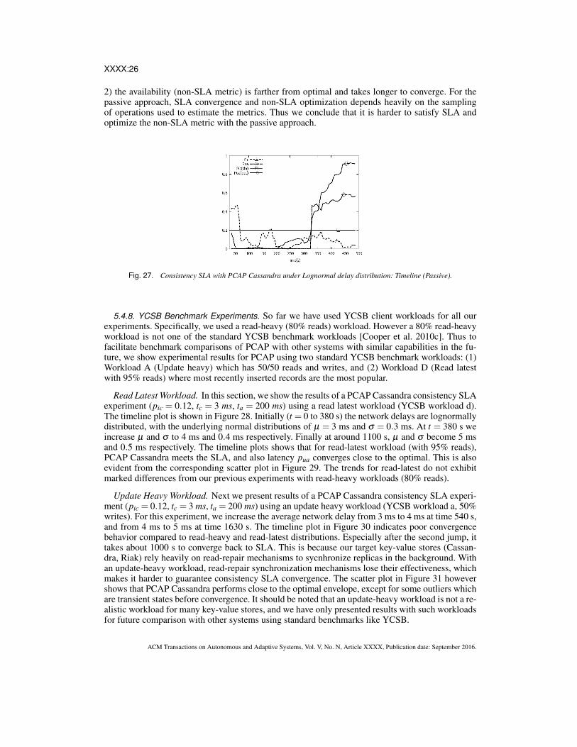
2) the availability (non-SLA metric) is farther from optimal and takes longer to converge. For thepassive approach, SLA convergence and non-SLA optimization depends heavily on the samplingof operations used to estimate the metrics. Thus we conclude that it is harder to satisfy SLA andoptimize the non-SLA metric with the passive approach.

Fig. 27. Consistency SLA with PCAP Cassandra under Lognormal delay distribution: Timeline (Passive).

5.4.8. YCSB Benchmark Experiments. So far we have used YCSB client workloads for all ourexperiments. Specifically, we used a read-heavy (80% reads) workload. However a 80% read-heavyworkload is not one of the standard YCSB benchmark workloads [Cooper et al. 2010c]. Thus tofacilitate benchmark comparisons of PCAP with other systems with similar capabilities in the fu-ture, we show experimental results for PCAP using two standard YCSB benchmark workloads: (1)Workload A (Update heavy) which has 50/50 reads and writes, and (2) Workload D (Read latestwith 95% reads) where most recently inserted records are the most popular.

Read Latest Workload. In this section, we show the results of a PCAP Cassandra consistency SLAexperiment (pic = 0.12, tc = 3 ms, ta = 200 ms) using a read latest workload (YCSB workload d).The timeline plot is shown in Figure 28. Initially (t = 0 to 380 s) the network delays are lognormallydistributed, with the underlying normal distributions of µ = 3 ms and σ = 0.3 ms. At t = 380 s weincrease µ and σ to 4 ms and 0.4 ms respectively. Finally at around 1100 s, µ and σ become 5 msand 0.5 ms respectively. The timeline plots shows that for read-latest workload (with 95% reads),PCAP Cassandra meets the SLA, and also latency pua converges close to the optimal. This is alsoevident from the corresponding scatter plot in Figure 29. The trends for read-latest do not exhibitmarked differences from our previous experiments with read-heavy workloads (80% reads).

Update Heavy Workload. Next we present results of a PCAP Cassandra consistency SLA experi-ment (pic = 0.12, tc = 3 ms, ta = 200 ms) using an update heavy workload (YCSB workload a, 50%writes). For this experiment, we increase the average network delay from 3 ms to 4 ms at time 540 s,and from 4 ms to 5 ms at time 1630 s. The timeline plot in Figure 30 indicates poor convergencebehavior compared to read-heavy and read-latest distributions. Especially after the second jump, ittakes about 1000 s to converge back to SLA. This is because our target key-value stores (Cassan-dra, Riak) rely heavily on read-repair mechanisms to sycnhronize replicas in the background. Withan update-heavy workload, read-repair synchronization mechanisms lose their effectiveness, whichmakes it harder to guarantee consistency SLA convergence. The scatter plot in Figure 31 howevershows that PCAP Cassandra performs close to the optimal envelope, except for some outliers whichare transient states before convergence. It should be noted that an update-heavy workload is not a re-alistic workload for many key-value stores, and we have only presented results with such workloadsfor future comparison with other systems using standard benchmarks like YCSB.

ACM Transactions on Autonomous and Adaptive Systems, Vol. V, No. N, Article XXXX, Publication date: September 2016.

XXXX:27

Fig. 28. Consistency SLA(tc = 3 ms, pic = 0.12, ta = 200 ms)with PCAP Cassandra under Lognormaldelay (latest) distribution: Timeline.

Fig. 29. Consistency SLA(tc = 3 ms, pic = 0.12, ta = 200 ms)with PCAP Cassandra under Lognormaldelay (latest) distribution: Scatter Plot.

Fig. 30. Consistency SLA(tc = 3 ms, pic = 0.12, ta = 200 ms)with PCAP Cassandra under Lognormaldelay (update-heavy) distribution: Timeline.

Fig. 31. Consistency SLA(tc = 3 ms, pic = 0.12, ta = 200 ms)with PCAP Cassandra under Lognormaldelay (update-heavy) distribution: Scatter Plot.

5.5. GeoPCAP EvaluationWe evaluate GeoPCAP with a Monte-Carlo simulation. In our setup, we have four data-centers,among which three are remote data-centers holding replicas of a key, and the fourth one is the localdata-center. At each iteration, we estimate t-freshness per data-center using a variation of the well-known WARS model [Bailis et al. 2014]. The WARS model is based on Dynamo style quorumsystems [DeCandia et al. 2007], where data staleness is due to read and write message reordering.The model has four components. W represents the message delay from coordinator to replica. Theacknowledgment from the replica back to the coordinator is modeled by a random variable A. Theread message delay from coordinator to replica, and the acknowledgment back are represented by R,and S, respectively. A read will be stale if a read is acknowledged before a write reaches the replica,

ACM Transactions on Autonomous and Adaptive Systems, Vol. V, No. N, Article XXXX, Publication date: September 2016.

XXXX:28

i. e. , R+ S < W +A. In our simulation, we ignore the A component since we do not need to waitfor a write to finish before a read starts. We use the LinkedIn SSD disk latency distribution [Bailiset al. 2014], Table 3 for read/write operation latency values.

We model the WAN delay using a normal distribution N(20 ms,√

2 ms) based on results from Bal-doni et al. [2006]. Each simulation runs for 300 iterations. At each iteration, we run the PID controlloop (Figure 9) to estimate a new value for geo-delay ∆, and sleep for 1 sec. All reads in the fol-lowing iteration are delayed at the local data-center by ∆. At iteration 150, we inject a jump byincreasing the mean and standard deviation of each WAN link delay normal distribution to 22 msand√

2.2 ms, respectively. We show only results for consistency and latency SLA for the ALL com-position. The QUICKEST composition results are similar and are omitted.

Fig. 32. GeoPCAP SLA Timeline for L SLA (ALL). Fig. 33. GeoPCAP SLA Timeline for C SLA (ALL).

Figure 32 shows the timeline of SLA convergence for GeoPCAP Latency SLA (pslaua =

0.27, tasla = 25 ms, tcsla = 0.1 ms). It should be noted that a latency SLA (pslaua = 0.27, tasla =

25 ms, tcsla = 0.1 ms) for GeoPCAP means that when using the ALL composition rule (all individ-ual data-center deployments must satisfy a latency deadline), each single data-center PCAP needsto provide an SLA specified as (psla

ua = 0.1, tasla = 25 ms, tcsla = 0.1 ms) (using the composition rulein the third row of Figure 6). We observe that using the PID controller (kp = 1, kd = 0.5, ki = 0.5),both the SLA and the other metric converge within 5 iterations initially and also after the jump.Figure 34 shows the corresponding evolution of the geo-delay control knob. Before the jump, theread delay converges to around 5 ms. After the jump, the WAN delay increase forces the geo-delayto converge to a lower value (around 3 ms) in order to meet the latency SLA.

Figure 33 shows the consistency SLA (pslaic = 0.38, tcsla = 1 ms, tasla = 25 ms) time line. Here

convergence takes 25 iterations, thanks to the PID controller ((kp = 1, kd = 0.8, ki = 0.5)). Weneeded a slightly higher value for the differential gain kd to deal with increased oscillation for theconsistency SLA experiment. Note that the psla

ic value of 0.38 forces a smaller per data-center picconvergence. The corresponding geo-delay evolution (Figure 35) initially converges to around 3 msbefore the jump, and converges to around 5 ms after the jump, to enforce the consistency SLA afterthe delay increase.

We also repeated the Latency SLA experiment with the ALL composition (Figures 32, 34) usingthe multiplicative control approach (Section 3.3) instead of the PID control approach. Figure 36shows the corresponding geo-delay trend compared to Figure 34. Comparing the two figures, weobserve that although the multiplicative strategy converges as fast the PID approach both beforeand after the delay jump, the read delay value keeps oscillating around the optimal value. Suchoscillations cannot be avoided in the multiplicative approach, since at steady state the control loop

ACM Transactions on Autonomous and Adaptive Systems, Vol. V, No. N, Article XXXX, Publication date: September 2016.

XXXX:29

Fig. 34. Geo-delay Timeline for L SLA (ALL)(Figure 32). Fig. 35. Geo-delay Timeline for C SLA (ALL)(Figure 33).

0

1

2

3

4

5

6

7

0 50 100 150 200 250 300

Geo

-del

ay

Iteration

Fig. 36. Geo-delay Timeline for A SLA (ALL) with Multiplicative Approach.

keeps changing direction with a unit step size. Compared to the multiplicative approach, the PIDcontrol approach is smoother and has less oscillations.

6. RELATED WORK6.1. Consistency-Latency TradeoffsIn addition to the Weak CAP Principle [Fox and Brewer 1999] and PACELC [Abadi 2012] discussedin Section 1, there has been work on theoretically characterizing the tradeoff between latency andstrong consistency models. Attiya and Welch Attiya and Welch [1994] studied the tradeoff betweenlatency and linearizability and sequential consistency. Subsequent work has explored linearizablityunder different delay models [Eleftheriou and Mavronicolas 1999; Mavronicolas and Roth 1999].All these papers are concerned with strong consistency models whereas we consider t-freshness,which models data freshness in eventually consistent systems. Moreover, their delay models aredifferent from our partition model. There has been theoretical work on probabilistic quorum sys-tems [Malkhi et al. 1997; Lee and Welch 2001; Abraham and Malkhi 2005]. Their consistencymodels are different from ours; moreover, they did not consider the tradeoff between consistencyand availability.

There are two classes of systems that are closest to our work. The first class of systems are con-cerned with metrics for measuring data freshness or staleness. We do not compare our work againstthis class of systems in this paper, as it is not our goal to propose yet another consistency model

ACM Transactions on Autonomous and Adaptive Systems, Vol. V, No. N, Article XXXX, Publication date: September 2016.

XXXX:30

or metric. Bailis et al. [2013, 2014] proposed a probabilistic consistency model (PBS) for quorum-based stores, but did not consider latency, soft partitions or the CAP theorem. Golab et al. [2011]proposed a time-based staleness metric called ∆-atomicity. ∆-atomicity is considered the gold stan-dard for measuring atomicity violations (staleness) across multiple read and write operations. TheΓ metric [Golab et al. 2014] is inspired by the ∆ metric and improves upon it on multiple fronts. Forexample, the Γ metric makes fewer technical assumptions than the ∆ metric and produces less noisyresults. It is also more robust against clock skew. All these related data freshness metrics cannot bedirectly compared to our t-freshness metric. The reason is that unlike our metric which considerswrite start times, these existing metrics consider end time of write operations when calculating datafreshness.

The second class of systems deal with adaptive mechanisms for meeting consistency-latencySLAs for key-value stores. The Pileus system [Terry et al. 2013] considered families of consis-tency/latency SLAs, and requires the application to specify a utility value with each SLA. In com-parison, PCAP considers probabilistic metrics of pic, pua. Tuba [Ardekani and Terry 2014] extendedthe predefined and static Pileus mechanisms with dynamic replica reconfiguration mechanisms tomaximize Pileus style utility functions without impacting client read and write operations. Golaband Wylie [2014] proposed consistency amplification, which is a framework for supporting consis-tency SLAs by injecting delays at servers or clients. In comparison, in our PCAP system, we onlyadd delays at servers. McKenzie et al. [2015] proposed continuous partial quorums (CPQ), whichis a technique to randomly choose between multiple discrete consistency levels for fine-grainedconsistency-latency tuning, and compare CPQ against consistency amplification. Compared to allthese systems where the goal is to meet SLAs, in our work, we also (1) quantitatively characterizethe (un)achievable consistency-latency tradeoff envelope, and (2) show how to design systems thatperform close to this envelope, in addition to (3) meeting SLAs. The PCAP system can be setup towork with any of these SLAs listed above; but we don’t do this in the paper since our main goal isto measure how close the PCAP system is to the optimal consistency-latency envelope.

Recently, there has been work on declarative ways to specify application consistency and latencyrequirements – PCAP proposes mechanisms to satisfy such specifications [Sivaramakrishnan et al.2015].

6.2. Adaptive SystemsThere are a few existing systems that controls consistency in storage systems. FRACS [Zhang andZhang 2003] controls consistency by allowing replicas to buffer updates up to a given staleness.AQuA [Krishnamurthy et al. 2003] continuously moves replicas between “strong” and “weak” con-sistency groups to implement different consistency levels. Fox and Brewer [1999] showed how totrade consistency (harvest) for availability (yield) in the context of the Inktomi search engine. Whileharvest and yield capture continuously changing consistency and availability conditions, we charac-terize the consistency-availability (latency) tradeoff in a quantitative manner. TACT [Yu and Vahdat2002] controls staleness by limiting the number of outstanding writes at replicas (order error) andbounding write propagation delay (staleness). All the mentioned systems provide best-effort behav-ior for consistency, within the latency bounds. In comparison, the PCAP system explicitly allowsapplications to specify SLAs. Consistency levels have been adaptively changed to deal with nodefailures and network changes in [Davidson et al. 2013], however this may be intrusive for appli-cations that explicitly set consistency levels for operations. Artificially delaying read operationsat servers (similar to our read delay knob) has been used to eliminate staleness spikes (improveconsistency) which are correlated with garbage collection in a specific key-value store (ApacheCassandra) [Fan et al. 2015]. Similar techniques have been used to guarantee causal consistency forclient-side applications [Zawirski et al. 2015]. Simba [Perkins et al. 2015] proposed new consis-tency abstractions for mobile application data synchronization services, and allows applications tochoose among various consistency models.

For stream processing, Gedik. et al. [2014] proposed a control algorithm to compute the op-timal resource requirements to meet throughput requirements. There has been work on adaptive

ACM Transactions on Autonomous and Adaptive Systems, Vol. V, No. N, Article XXXX, Publication date: September 2016.

XXXX:31

elasticity control for storage [Lim et al. 2010], and adaptively tuning Hadoop clusters to meetSLAs [Herodotou et al. 2011]. Compared to the controllers present in these systems, our PCAPcontroller achieves control objectives [Hellerstein et al. 2004] using a different set of techniques tomeet SLAs for key-value stores.

6.3. CompositionComposing local policies to form global policies is well studied in other domains, for example QoScomposition in multimedia networks [Liang and Nahrstedt 2006], software defined network (sdn)composition [Monsanto et al. 2013], and web-service orchestration [Dustdar and Schreiner 2005].Our composition techniques are aimed at consistency and latency guarantees for geo-distributedsystems.

7. SUMMARYIn this paper, we have first formulated and proved a probabilistic variation of the CAP theoremwhich took into account probabilistic models for consistency, latency, and soft partitions within adata-center. Our theorems show the un-achievable envelope, i.e., which combinations of these threemodels make them impossible to achieve together. We then showed how to design systems (calledPCAP) that (1) perform close to this optimal envelope, and (2) can meet consistency and latencySLAs derived from the corresponding models. We then incorporated these SLAs into Apache Cas-sandra and Riak running in a single data-center. We also extended our PCAP system from a singledata-center to multiple geo-distributed data-centers. Our experiments with YCSB workloads andrealistic traffic demonstrated that our PCAP system meets the SLAs, that its performance is close tothe optimal-achievable consistency-availability envelope, and that it scales well. Simulations of ourGeoPCAP system also showed SLA satisfaction for applications spanning multiple data-centers.

REFERENCES

Daniel Abadi. 2012. Consistency Tradeoffs in Modern Distributed Database System Design: CAPis Only Part of the Story. IEEE Computer 45, 2 (2012), 37–42.

Ittai Abraham and Dahlia Malkhi. 2005. Probabilistic quorums for dynamic systems. DistributedComputing 18, 2 (2005), 113–124.

Masoud Saeida Ardekani and Douglas B. Terry. 2014. A Self-configurable Geo-replicated CloudStorage System. In Proceedings of the 11th USENIX Conference on Operating Systems Designand Implementation (OSDI). Broomfield, CO, USA, 367–381.

K. J. Astrom and T. Hagglund. 1995. PID Controllers: Theory, Design, and Tuning, 2nd Ed. TheInstrument, Systems, and Automation Society, Research Triangle Park, NC.

Hagit Attiya and Jennifer L. Welch. 1994. Sequential Consistency Versus Linearizability. ACMTransactions on Computer Systems (TOCS) 12, 2 (1994), 91–122.

Peter Bailis and Ali Ghodsi. 2013. Eventual Consistency Today: Limitations, Extensions, and Be-yond. ACM Queue 11, 3 (2013), 20:20–20:32.

Peter Bailis, Shivaram Venkataraman, Michael J. Franklin, JosephM. Hellerstein, and Ion Stoica.2014. Quantifying eventual consistency with PBS. The Very Large Data Bases (VLDB) Journal23, 2 (2014), 279–302.

Peter Bailis, Shivaram Venkataraman, Michael J. Franklin, Joseph M. Hellerstein, and Ion Stoica.2013. PBS at Work: Advancing Data Management with Consistency Metrics. In Proceedingsof the 2013 ACM SIGMOD International Conference on Management of Data (SIGMOD). NewYork, New York, USA, 1113–1116.

R. Baldoni, C. Marchetti, and A. Virgillito. 2006. Impact of WAN Channel Behavior on End-to-end Latency of Replication Protocols. In Proceedings of European Dependable ComputingConference (EDCC). Coimbra, Portugal, 109–118.

Jeff Barr. 2013. Real-time ad impression bids using DynamoDB. http://goo.gl/C7gdpc.

ACM Transactions on Autonomous and Adaptive Systems, Vol. V, No. N, Article XXXX, Publication date: September 2016.

XXXX:32

Theophilus Benson, Aditya Akella, and David A. Maltz. 2010. Network Traffic Characteristics ofDatacenters in the Wild. In Proceedings of the 10th ACM SIGCOMM Conference on InternetMeasurement (IMC). Melbourne, Australia, 267–280.

Eric Brewer. 2000. Towards robust distributed systems (Abstract). In Proceedings of the NineteenthAnnual ACM Symposium on Principles of Distributed Computing (PODC). Portland, Oregon,USA.

Eric Brewer. 2010. A Certain Freedom: Thoughts on the CAP Theorem. In Proceedings of the 29thACM SIGACT-SIGOPS Symposium on Principles of Distributed Computing (PODC). Zurich,Switzerland, 335–335.

Adrian Cockcroft. 2013. Dystopia as a Service (Invited Talk). In Proceedings of the 4th AnnualSymposium on Cloud Computing (SoCC). Santa Clara, California.

Brian F. Cooper, Adam Silberstein, Erwin Tam, Raghu Ramakrishnan, and Russell Sears. 2010a.Benchmarking cloud serving systems with YCSB. In Proceedings of the 1st ACM Symposium onCloud Computing (SoCC). Indianapolis, Indiana, USA, 143–154.

Brian F. Cooper, Adam Silberstein, Erwin Tam, Raghu Ramakrishnan, and Russell Sears. 2010b.Yahoo! Cloud Serving Benchmark (YCSB). http://goo.gl/GiA5c.

Brian F. Cooper, Adam Silberstein, Erwin Tam, Raghu Ramakrishnan, and Russell Sears. 2010c.Yahoo! Cloud Serving Benchmark (YCSB) Workloads. https://github.com/brianfrankcooper/YCSB/wiki/Core-Workloads.

James C. Corbett, Jeffrey Dean, Michael Epstein, Andrew Fikes, Christopher Frost, J. J. Furman,Sanjay Ghemawat, Andrey Gubarev, Christopher Heiser, Peter Hochschild, Wilson Hsieh, Sebas-tian Kanthak, Eugene Kogan, Hongyi Li, Alexander Lloyd, Sergey Melnik, David Mwaura, DavidNagle, Sean Quinlan, Rajesh Rao, Lindsay Rolig, Yasushi Saito, Michal Szymaniak, ChristopherTaylor, Ruth Wang, and Dale Woodford. 2012. Spanner: Google’s Globally-distributed Database.In Proceedings of the 10th USENIX Conference on Operating Systems Design and Implementa-tion (OSDI). Hollywood, CA, USA, 251–264.

DataStax. 2016. Configuring Data Consistency. https://goo.gl/PKNUXVAaron Davidson, Aviad Rubinstein, Anirudh Todi, Peter Bailis, and Shivaram Venkataraman. 2013.

Adaptive Hybrid Quorums in Practical Settings. http://goo.gl/LbRSW3.Jeff Dean. 2009. Design, Lessons and Advice from Building Large Distributed Systems. (2009).

http://goo.gl/HGJqUh.Giuseppe DeCandia, Deniz Hastorun, Madan Jampani, Gunavardhan Kakulapati, Avinash Laksh-

man, Alex Pilchin, Swaminathan Sivasubramanian, Peter Vosshall, and Werner Vogels. 2007. Dy-namo: Amazon’s Highly Available Key-value Store. In Proceedings of Twenty-first ACM SIGOPSSymposium on Operating Systems Principles (SOSP). Stevenson, Washington, USA, 205–220.

Schahram Dustdar and Wolfgang Schreiner. 2005. A Survey on Web Services Composition. Inter-national Journal of Web and Grid Services 1, 1 (2005), 1–30.

Maria Eleftheriou and Marios Mavronicolas. 1999. Linearizability in the Presence of DriftingClocks and Under Different Delay Assumptions. In Distributed Computing. Vol. 1693. 327–341.

Hua Fan, Aditya Ramaraju, Marlon McKenzie, Wojciech Golab, and Bernard Wong. 2015. Un-derstanding the Causes of Consistency Anomalies in Apache Cassandra. Proceedings of the VeryLarge Data Bases (VLDB) Endowment 8, 7 (2015), 810–813.

Armando Fox and Eric A. Brewer. 1999. Harvest, Yield, and Scalable Tolerant Systems. In Pro-ceedings of the The Seventh Workshop on Hot Topics in Operating Systems (HotOS). Rio Rico,Arizona, USA, 174–178.

Bugra Gedik., Scott Schneider, Martin Hirzel, and Kun-Lung Wu. 2014. Elastic Scaling for DataStream Processing. IEEE Transactions on Parallel and Distributed Systems (TPDS) 25, 6 (2014),1447–1463.

Seth Gilbert and Nancy Lynch. 2002. Brewer’s Conjecture and the Feasibility of Consistent, Avail-able, Partition-tolerant Web Services. ACM SIGACT News 33, 2 (2002), 51–59.

Seth Gilbert and Nancy Lynch. 2012. Perspectives on the CAP Theorem. IEEE Computer 45, 2(2012), 30–36.

ACM Transactions on Autonomous and Adaptive Systems, Vol. V, No. N, Article XXXX, Publication date: September 2016.

XXXX:33

Eric Gilmore. 2011. Cassandra Multi data-center deployment. http://goo.gl/aA8YIS.Lisa Glendenning, Ivan Beschastnikh, Arvind Krishnamurthy, and Thomas Anderson. 2011. Scal-

able Consistency in Scatter. In Proceedings of the Twenty-Third ACM Symposium on OperatingSystems Principles (SOSP). Cascais, Portugal, 15–28.

Wojciech Golab, Xiaozhou Li, and Mehul A. Shah. 2011. Analyzing consistency properties for funand profit. In Proceedings of the 30th Annual ACM SIGACT-SIGOPS Symposium on Principlesof Distributed Computing (PODC). San Jose, California, USA, 197–206.

Wojciech Golab, Muntasir Raihan Rahman, Alvin AuYoung, Kimberly Keeton, and Indranil Gupta.2014. Client-Centric Benchmarking of Eventual Consistency for Cloud Storage Systems. InProceedings of the 2014 IEEE 34th International Conference on Distributed Computing Systems(ICDCS). Madrid, Spain.

Wojciech Golab and John Johnson Wylie. 2014. Providing A Measure Representing an Instanta-neous Data Consistency Level. (Jan. 2014). US Patent Application 20,140,032,504.

Andy Gross. 2009. Basho Riak. http://basho.com/riak/.Joseph L. Hellerstein, Yixin Diao, Sujay Parekh, and Dawn M. Tilbury. 2004. Feedback Control of

Computing Systems. John Wiley & Sons.Herodotos Herodotou, Fei Dong, and Shivnath Babu. 2011. No One (Cluster) Size Fits All: Auto-

matic Cluster Sizing for Data-intensive Analytics. In Proceedings of the 2nd ACM Symposium onCloud Computing (SoCC). Cascais, Portugal, 18:1–18:14.

Sudha Krishnamurthy, William H. Sanders, and Michel Cukier. 2003. An Adaptive Quality of Ser-vice Aware Middleware for Replicated Services. IEEE Transactions on Parallel and DistributedSystems (TPDS) 14 (2003), 1112–1125.

Avinash Lakshman and Prashant Malik. 2008. Apache Cassandra. http://cassandra.apache.org/.Keith Lang. 2009. Amazon: milliseconds means money. http://goo.gl/fs9pZb.Hyunyoung Lee and Jennifer L. Welch. 2001. Applications of Probabilistic Quorums to Iterative

Algorithms. In Proceedings of the The 21st International Conference on Distributed ComputingSystems (ICDCS). Phoenix (Mesa), Arizona, USA, 21.

Cheng Li, Daniel Porto, Allen Clement, Johannes Gehrke, Nuno Preguica, and Rodrigo Rodrigues.2012. Making Geo-replicated Systems Fast As Possible, Consistent when Necessary. In Proceed-ings of the 10th USENIX Conference on Operating Systems Design and Implementation (OSDI).Hollywood, CA, USA, 265–278.

Jin Liang and Klara Nahrstedt. 2006. Service Composition for Generic Service Graphs. MultimediaSystems 11, 6 (2006), 568–581.

Harold C. Lim, Shivnath Babu, and Jeffrey S. Chase. 2010. Automated Control for Elastic Storage.In Proceedings of the 7th International Conference on Autonomic Computing (ICAC). Washing-ton, DC, USA, 1–10.

LinkedIn. 2009. Project Voldemort. http://goo.gl/9uhLoUWyatt Lloyd, Michael J. Freedman, Michael Kaminsky, and David G. Andersen. 2011. Don’t Settle

for Eventual: Scalable Causal Consistency for Wide-Area Storage with COPS. In Proceedings ofthe Twenty-Third ACM Symposium on Operating Systems Principles (SOSP). Cascais, Portugal,401–416.

Wyatt Lloyd, Michael J. Freedman, Michael Kaminsky, and David G. Andersen. 2013. StrongerSemantics for Low-Latency Geo-Replicated Storage. In Proceedings of the 10th USENIX Con-ference on Networked Systems Design and Implementation (NSDI). Lombard, IL, USA, 313–328.

Dahlia Malkhi, Michael Reiter, and Rebecca Wright. 1997. Probabilistic Quorum Systems. InProceedings of the Sixteenth Annual ACM Symposium on Principles of Distributed Computing(PODC). Santa Barbara, California, USA, 267–273.

Marios Mavronicolas and Dan Roth. 1999. Linearizable Read/Write Objects. Theoretical ComputerScience 220, 1 (1999), 267 – 319.

Marlon McKenzie, Hua Fan, and Wojciech Golab. 2015. Fine-tuning the Consistency-latency Trade-off in Quorum-replicated Distributed Storage Systems. In Proceedings of the 2015 IEEE Interna-tional Conference on Big Data. Santa Clara, CA, USA, 1708–1717.

ACM Transactions on Autonomous and Adaptive Systems, Vol. V, No. N, Article XXXX, Publication date: September 2016.

XXXX:34

Christopher Monsanto, Joshua Reich, Nate Foster, Jennifer Rexford, and David Walker. 2013.Composing Software-defined Networks. In Proceedings of the 10th USENIX Conference on Net-worked Systems Design and Implementation (NSDI). Lombard, IL, USA, 1–14.

Ron Peled. 2010. Activo: “Why Low Latency Matters?”. http://goo.gl/2XQ8UlDorian Perkins, Nitin Agrawal, Akshat Aranya, Curtis Yu, Younghwan Go, Harsha V. Madhyastha,

and Cristian Ungureanu. 2015. Simba: Tunable End-to-end Data Consistency for Mobile Apps.In Proceedings of the Tenth European Conference on Computer Systems (EuroSys). Bordeaux,France, 7:1–7:16.

Marc Shapiro. 1986. Structure and Encapsulation in Distributed Systems: the Proxy Principle. InProc. International Conference on Distributed Computing Systems (ICDCS). Cambridge, MA,USA, 198–204.

Marc Shapiro, Nuno M. Preguica, Carlos Baquero, and Marek Zawirski. 2011. Conflict-Free Repli-cated Data Types. In Proceedings of the 13th International Conference on Stabilization, Safety,and Security of Distributed Systems (SSS). Grenoble, France, 386–400.

K. C. Sivaramakrishnan, Gowtham Kaki, and Suresh Jagannathan. 2015. Declarative ProgrammingOver Eventually Consistent Data Stores. In Proceedings of the 36th ACM SIGPLAN Conferenceon Programming Language Design and Implementation (PLDI). Portland, OR, USA, 413–424.

Ion Stoica, Robert Morris, David Karger, M. Frans Kaashoek, and Hari Balakrishnan. 2001. Chord:A Scalable Peer-to-peer Lookup Service for Internet Applications. In Proceedings of the 2001Conference on Applications, Technologies, Architectures, and Protocols for Computer Commu-nications (SIGCOMM). San Diego, California, USA, 149–160.

Shlomo Swidler. 2009. Consistency in Amazon S3. http://goo.gl/yhAoJy.Douglas B. Terry, Vijayan Prabhakaran, Ramakrishna Kotla, Mahesh Balakrishnan, Marcos K.

Aguilera, and Hussam Abu-Libdeh. 2013. Consistency-based Service Level Agreements forCloud Storage. In Proceedings of the Twenty-Fourth ACM Symposium on Operating SystemsPrinciples (SOSP). Farminton, Pennsylvania, USA, 309–324.

Werner Vogels. 2009. Eventually Consistent. Communications of the ACM (CACM) (2009), 40–44.Hengfeng Wei, Yu Huang, Jiannong Cao, and Jian Lu. 2015. Almost Strong Consistency: ”Good

Enough” in Distributed Storage Systems. http://arxiv.org/abs/1507.01663.Brian White, Jay Lepreau, Leigh Stoller, Robert Ricci, Shashi Guruprasad, Mac Newbold, Mike

Hibler, Chad Barb, and Abhijeet Joglekar. 2002. An Integrated Experimental Environment forDistributed Systems and Networks. In Proceedings of the Fifth Symposium on Operating SystemsDesign and Implementation (OSDI). Boston, Massachusetts, 255–270.

Haifeng Yu and Amin Vahdat. 2002. Design and Evaluation of a Conit-based Continuous Con-sistency Model for Replicated Services. ACM Transactions on Computer Systems (TOCS) 20, 3(2002), 239–282.

Marek Zawirski, Nuno Preguica, Sergio Duarte, Annette Bieniusa, Valter Balegas, and MarcShapiro. 2015. Write Fast, Read in the Past: Causal Consistency for Client-Side Applications. InProceedings of the 16th Annual Middleware Conference. Vancouver, BC, Canada, 75–87.

Chi Zhang and Zheng Zhang. 2003. Trading Replication Consistency for Performance and Avail-ability: an Adaptive Approach. In Proceedings of the 23rd International Conference on Dis-tributed Computing Systems (ICDCS). Providence, Rhode Island, USA, 687–695.

ACM Transactions on Autonomous and Adaptive Systems, Vol. V, No. N, Article XXXX, Publication date: September 2016.